
Assessment of Artificial Intelligence Strategies to Estimate the Strength of Geopolymer Composites and Influence of Input Parameters

 , , ,
, , ,
Abstract
:1. Introduction
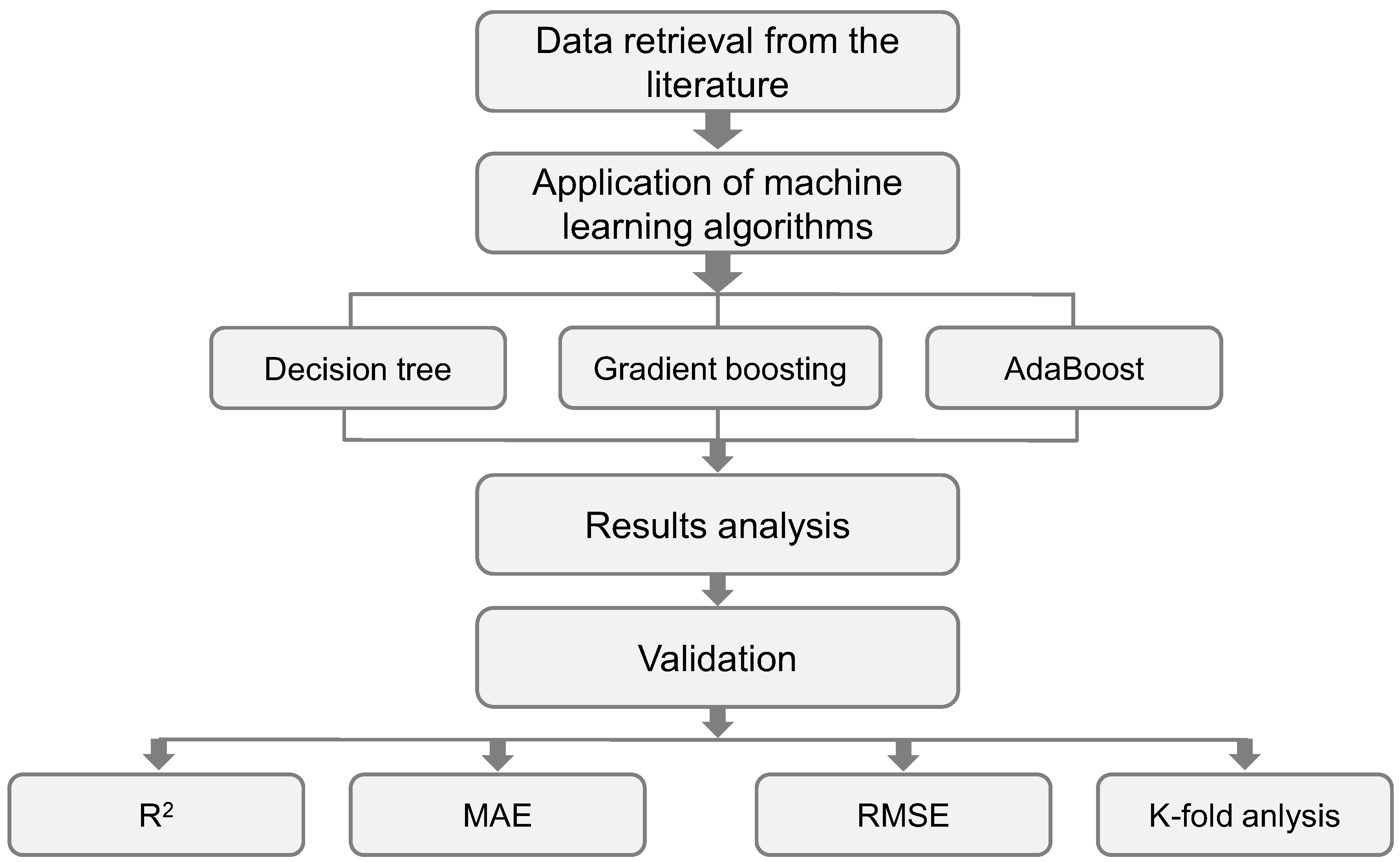
2. Methods
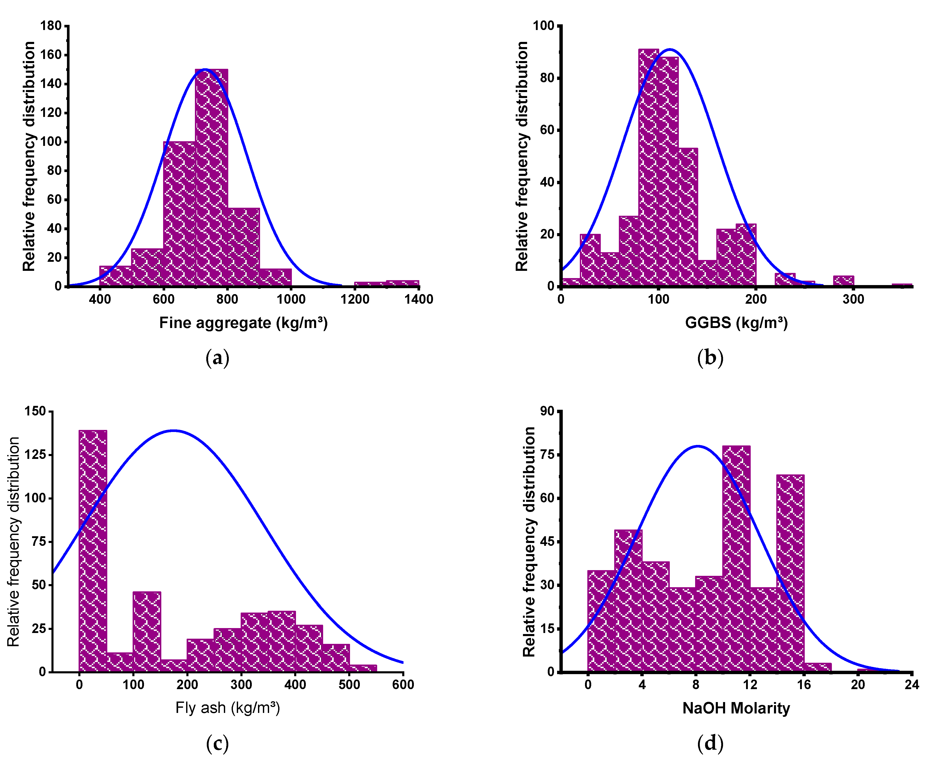
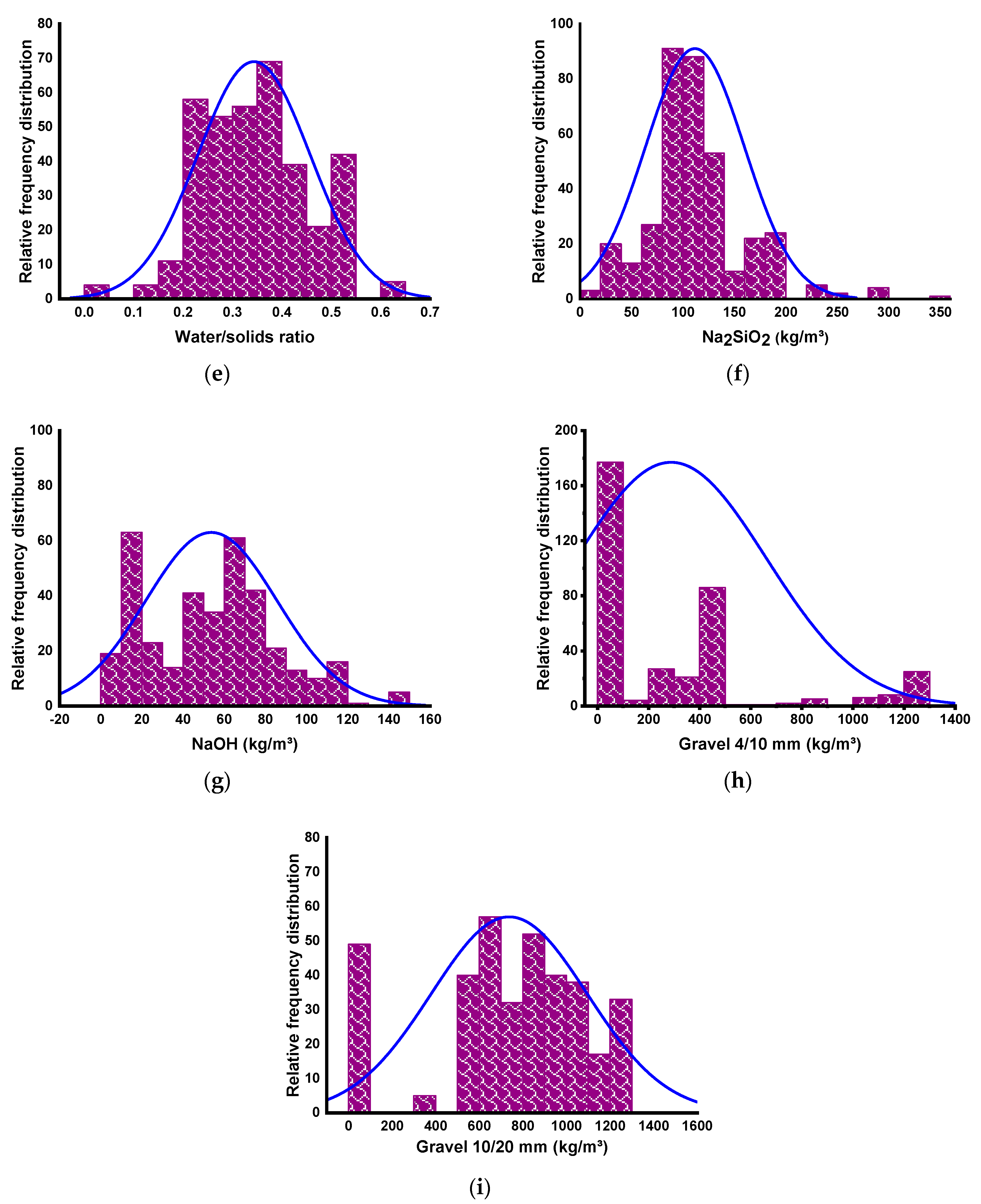
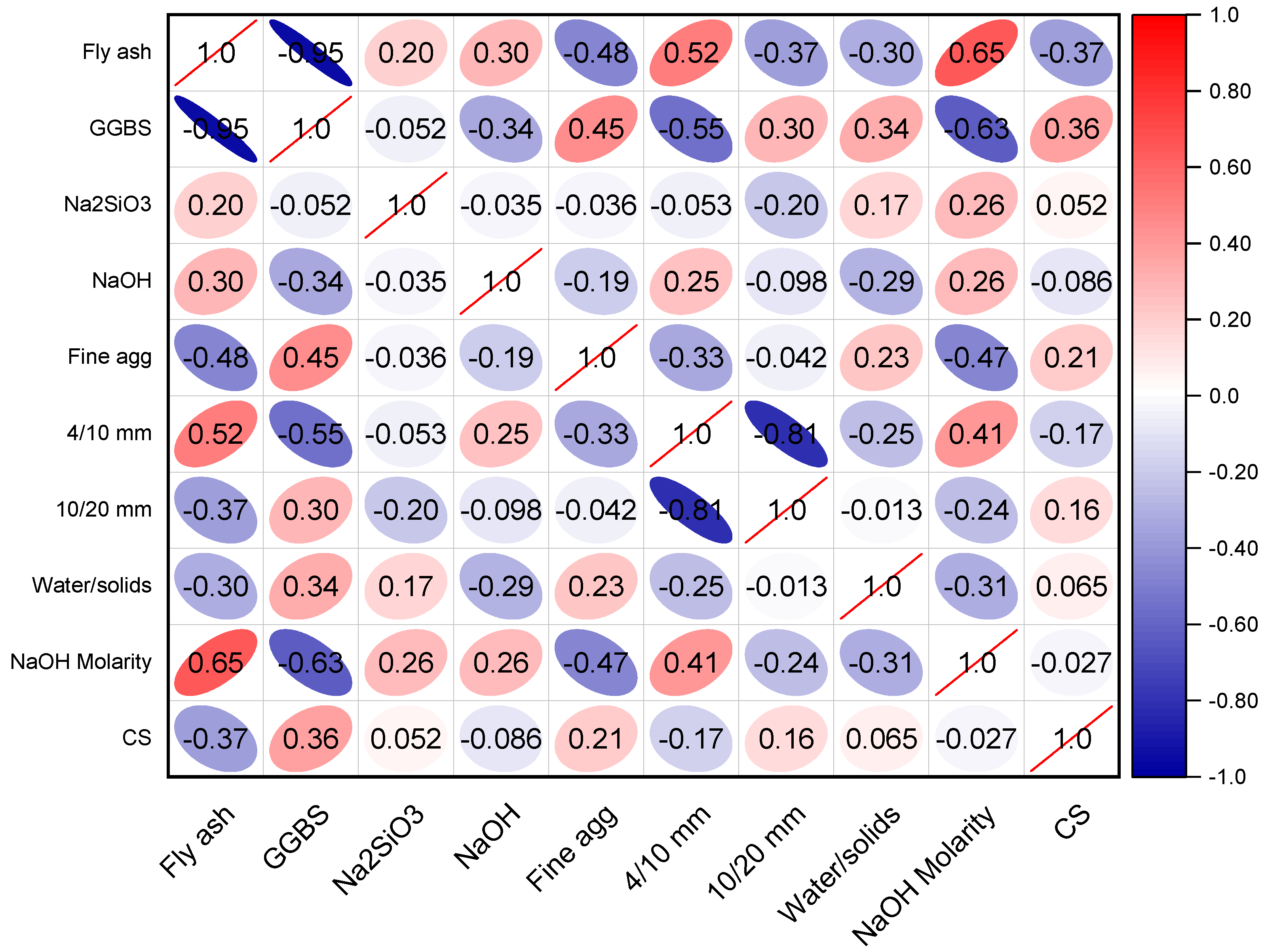
2.1. Data Retrieval and Analysis
2.2. Machine Learning Algorithms Employed
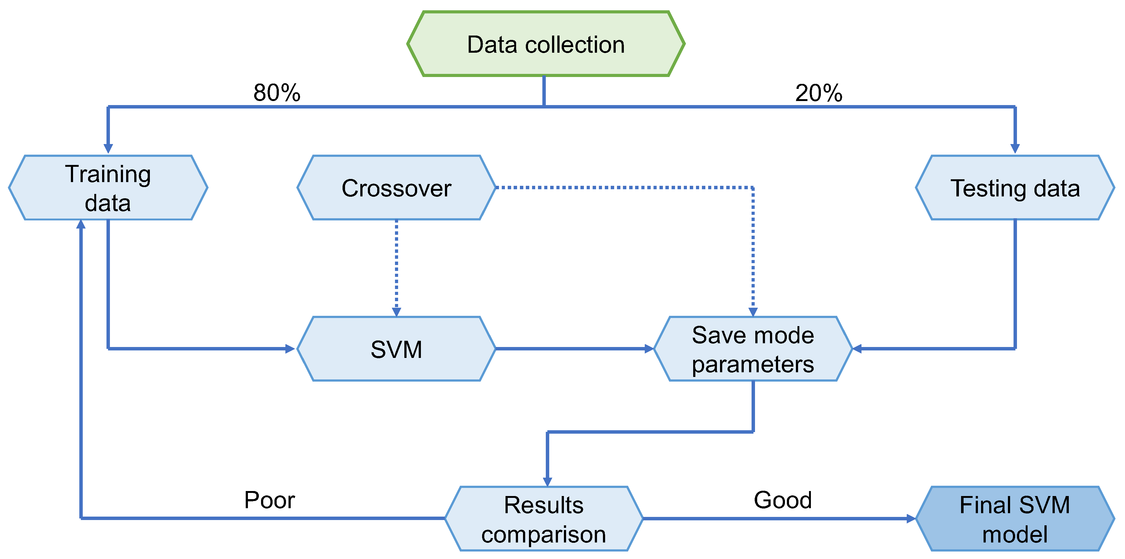
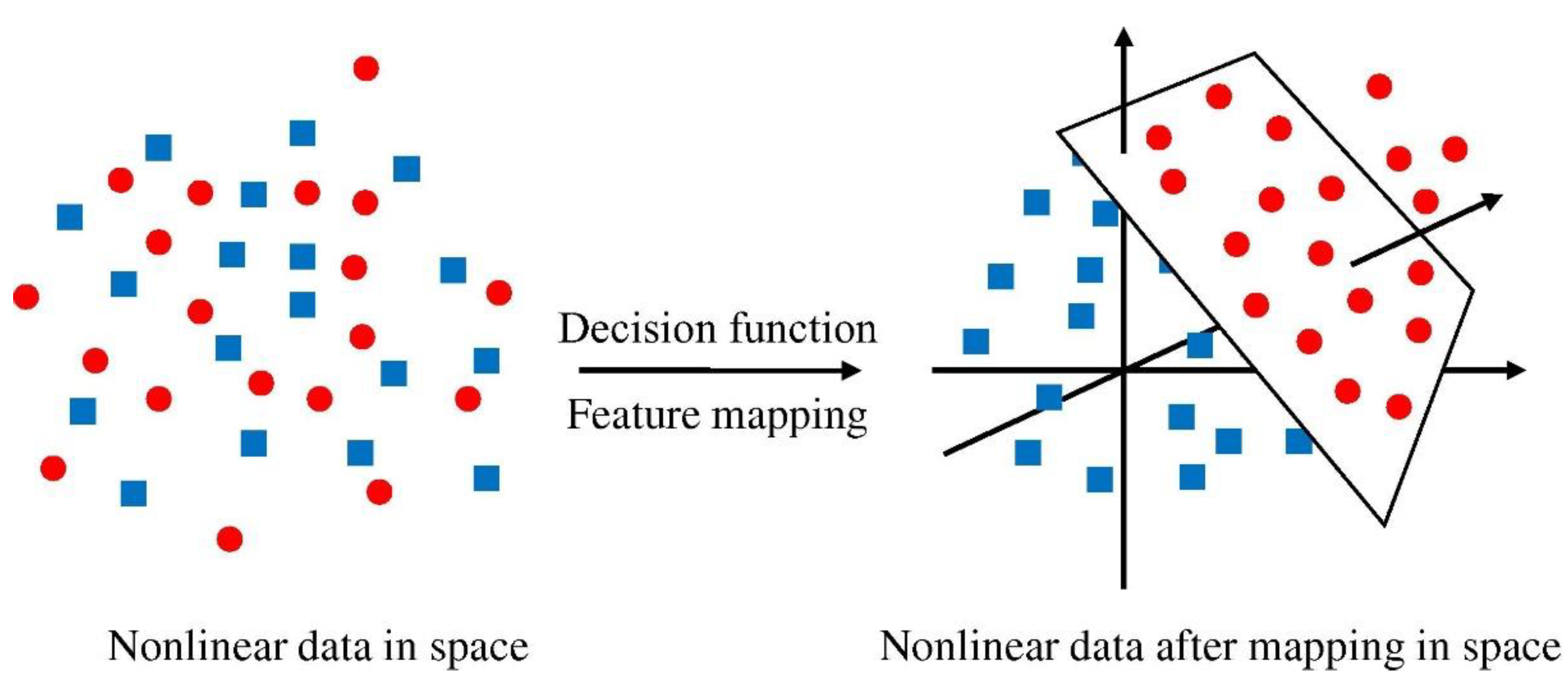
2.2.1. Support Vector Machine
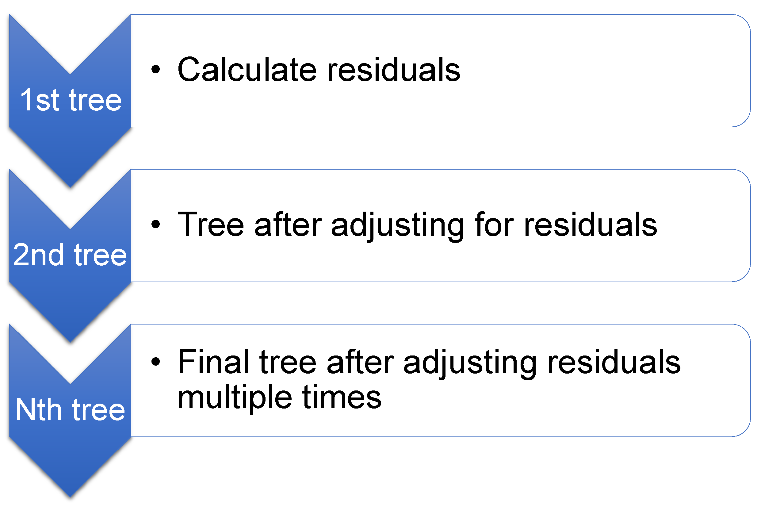
2.2.2. Gradient Boosting
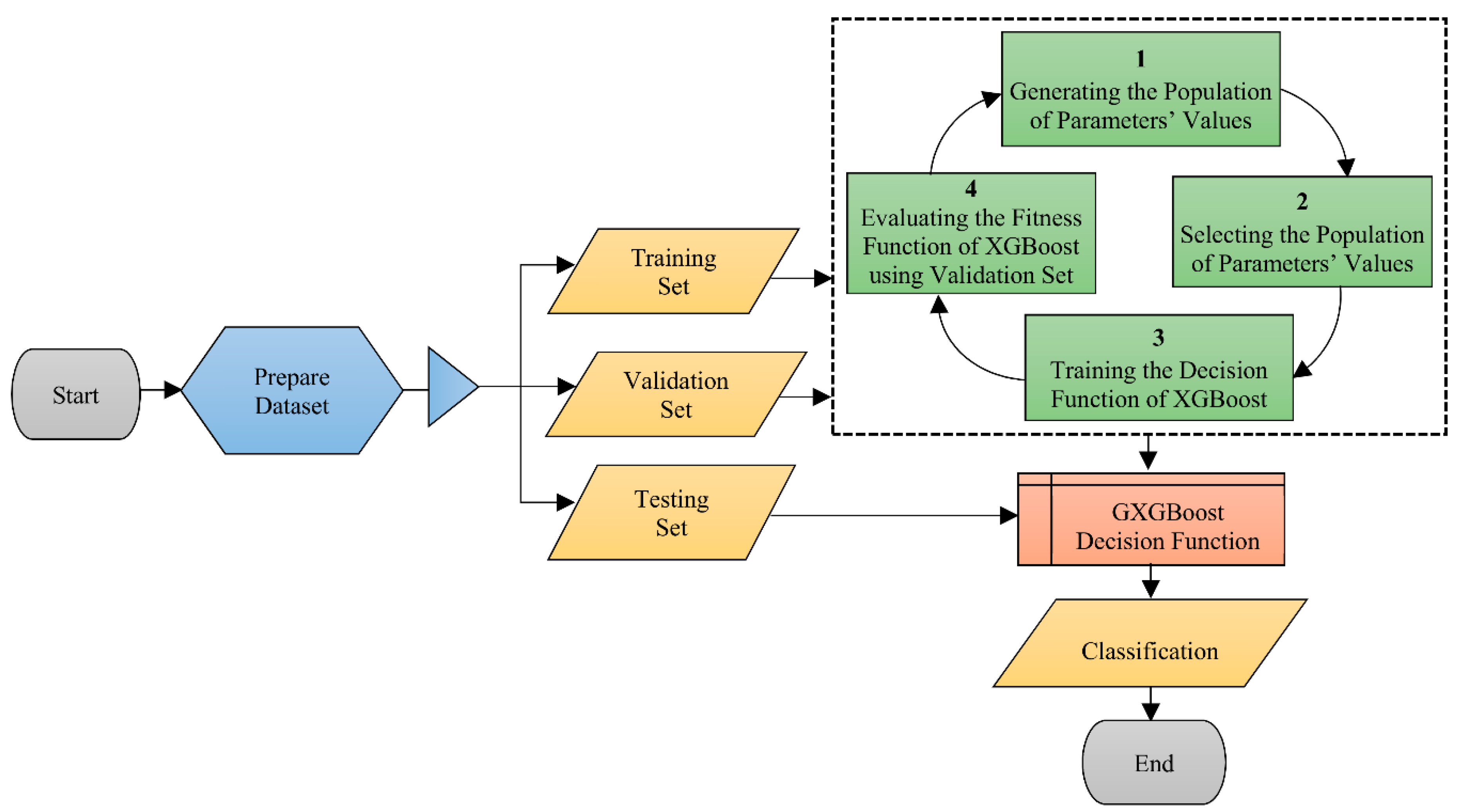
2.2.3. Extreme Gradient Boosting
3. Analysis of Results
3.1. Support Vector Machine Model
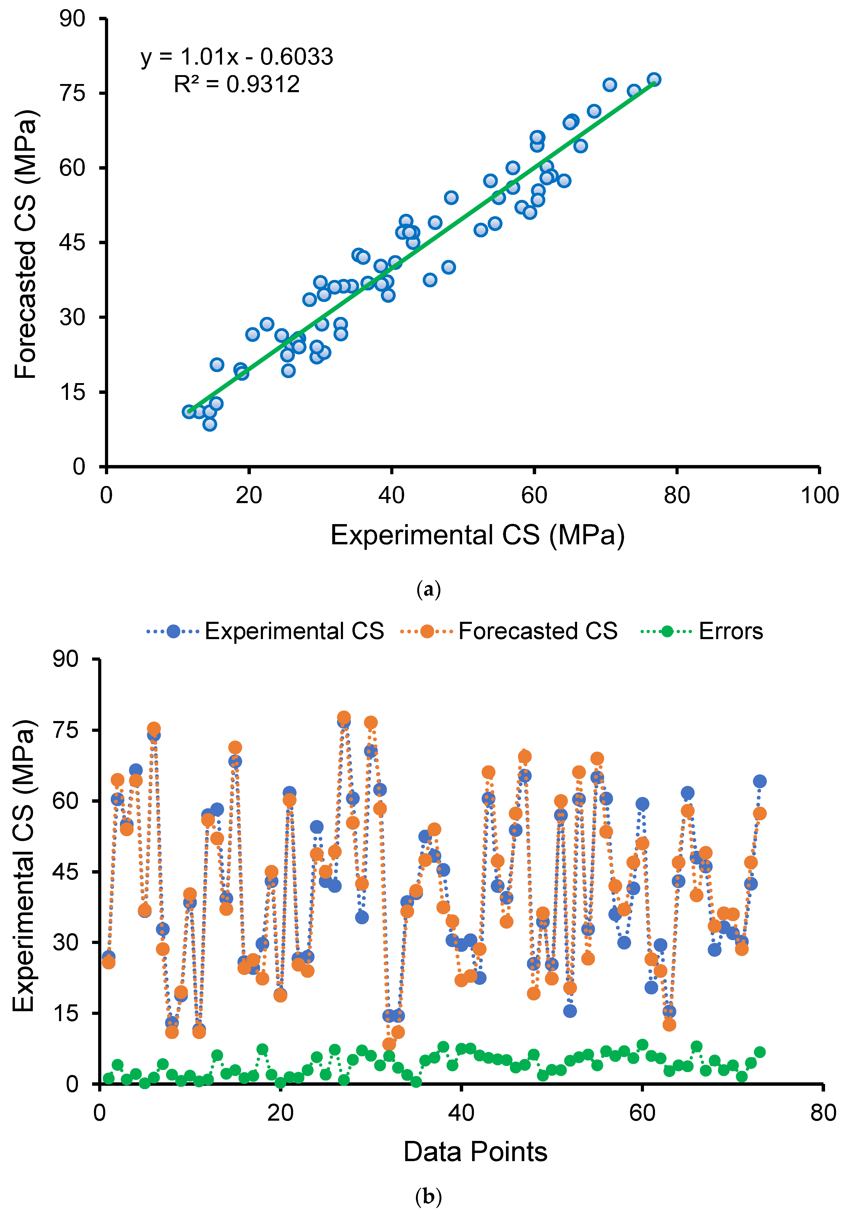
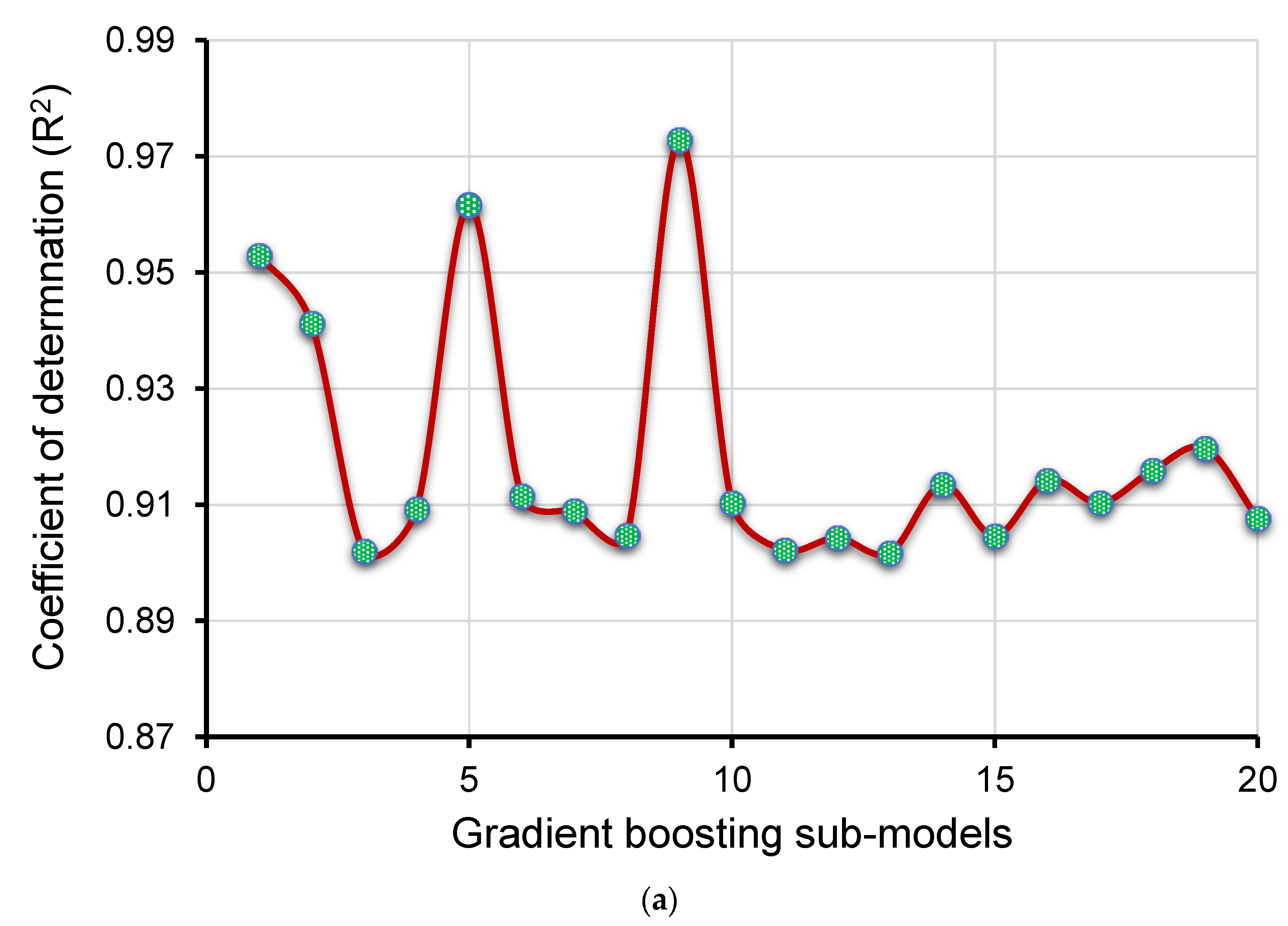
3.2. Gradient Boosting Model
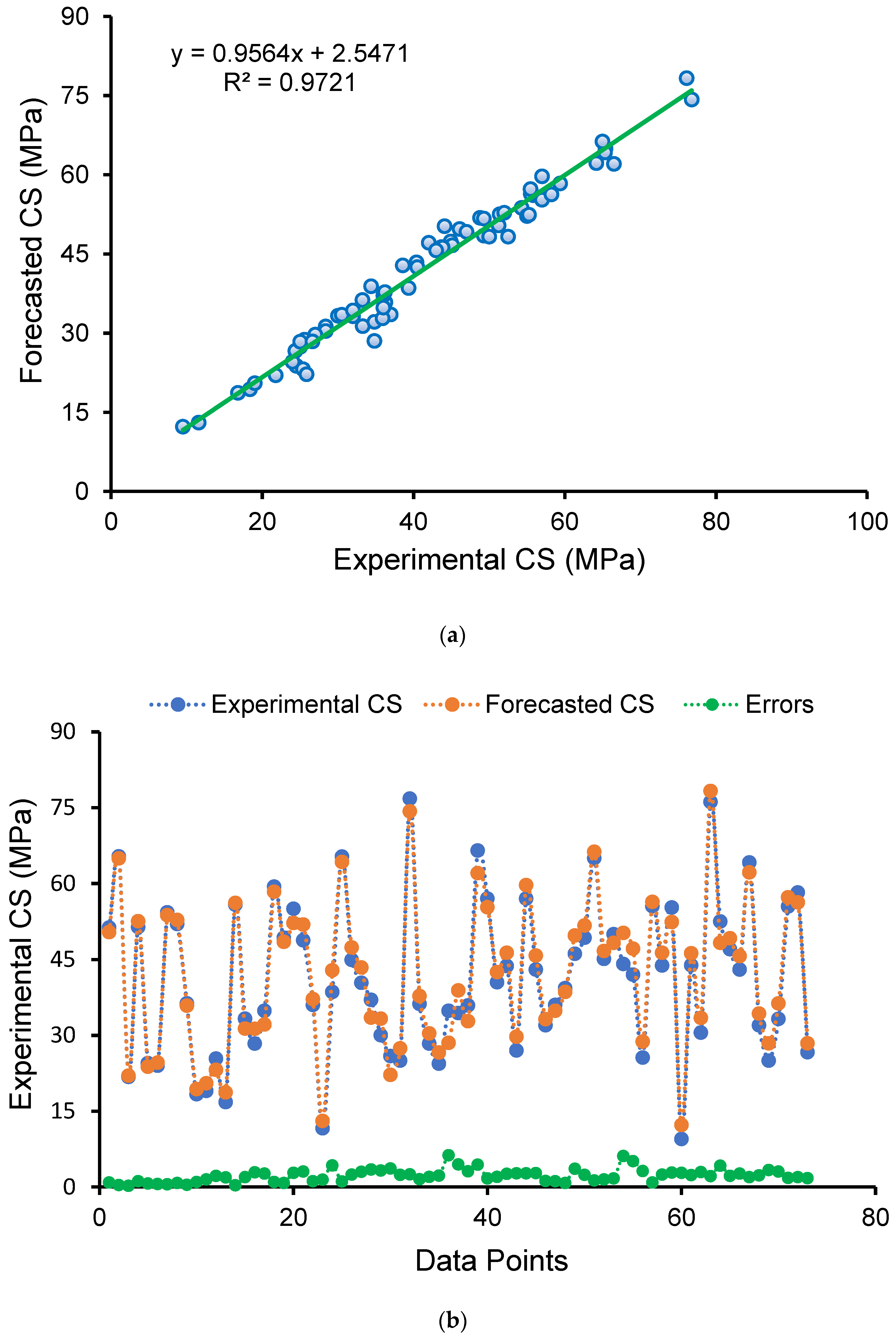
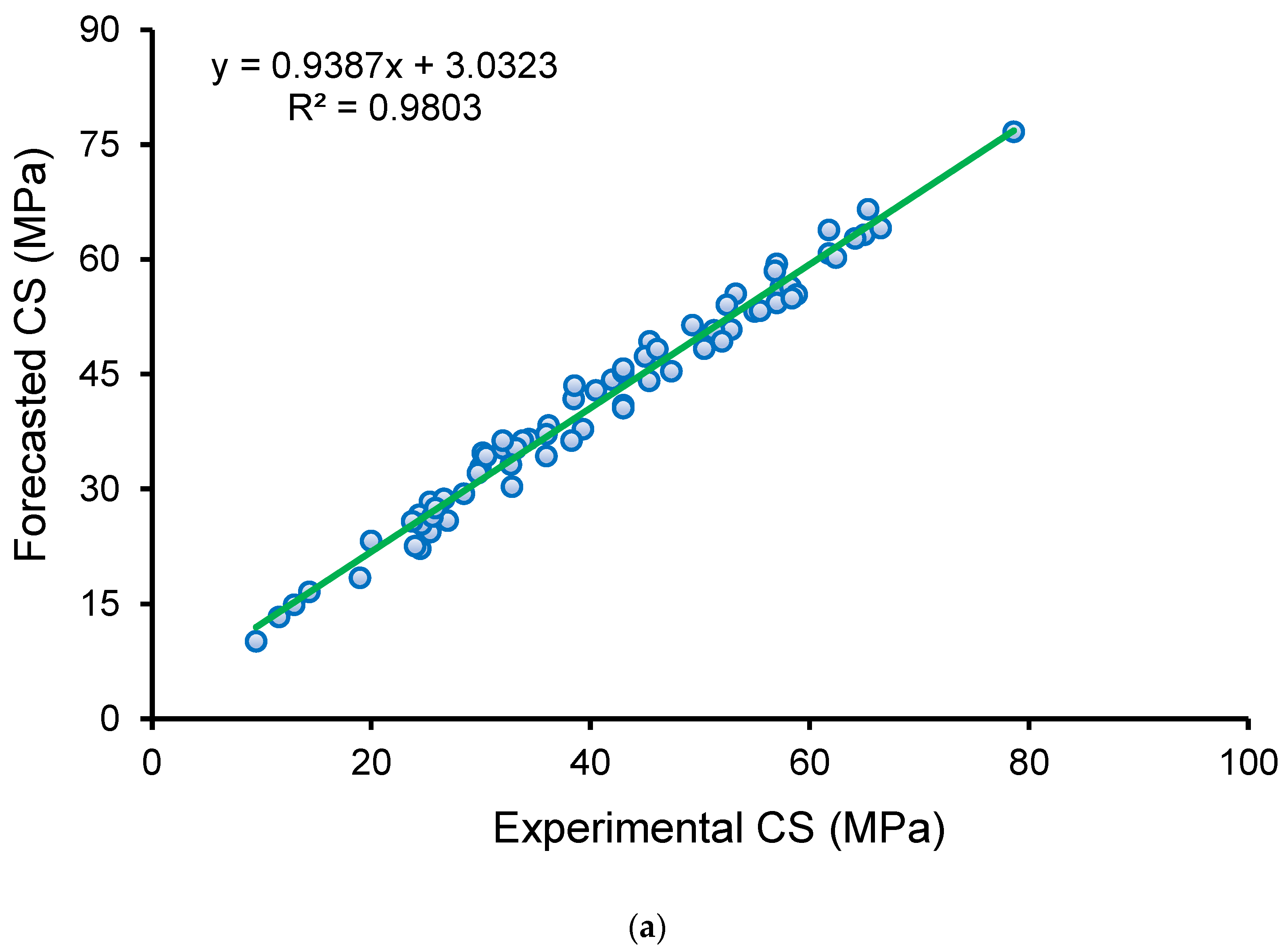
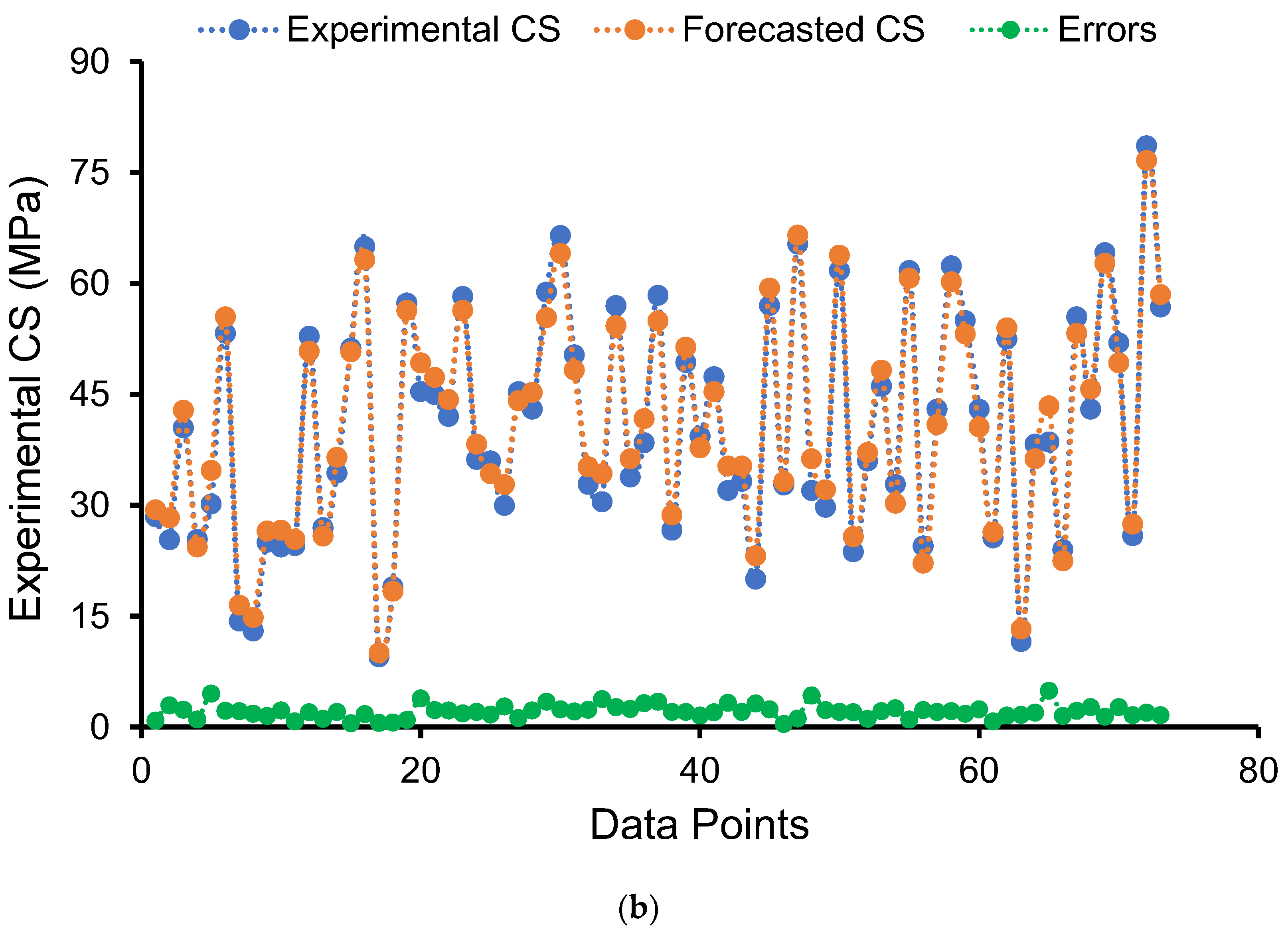
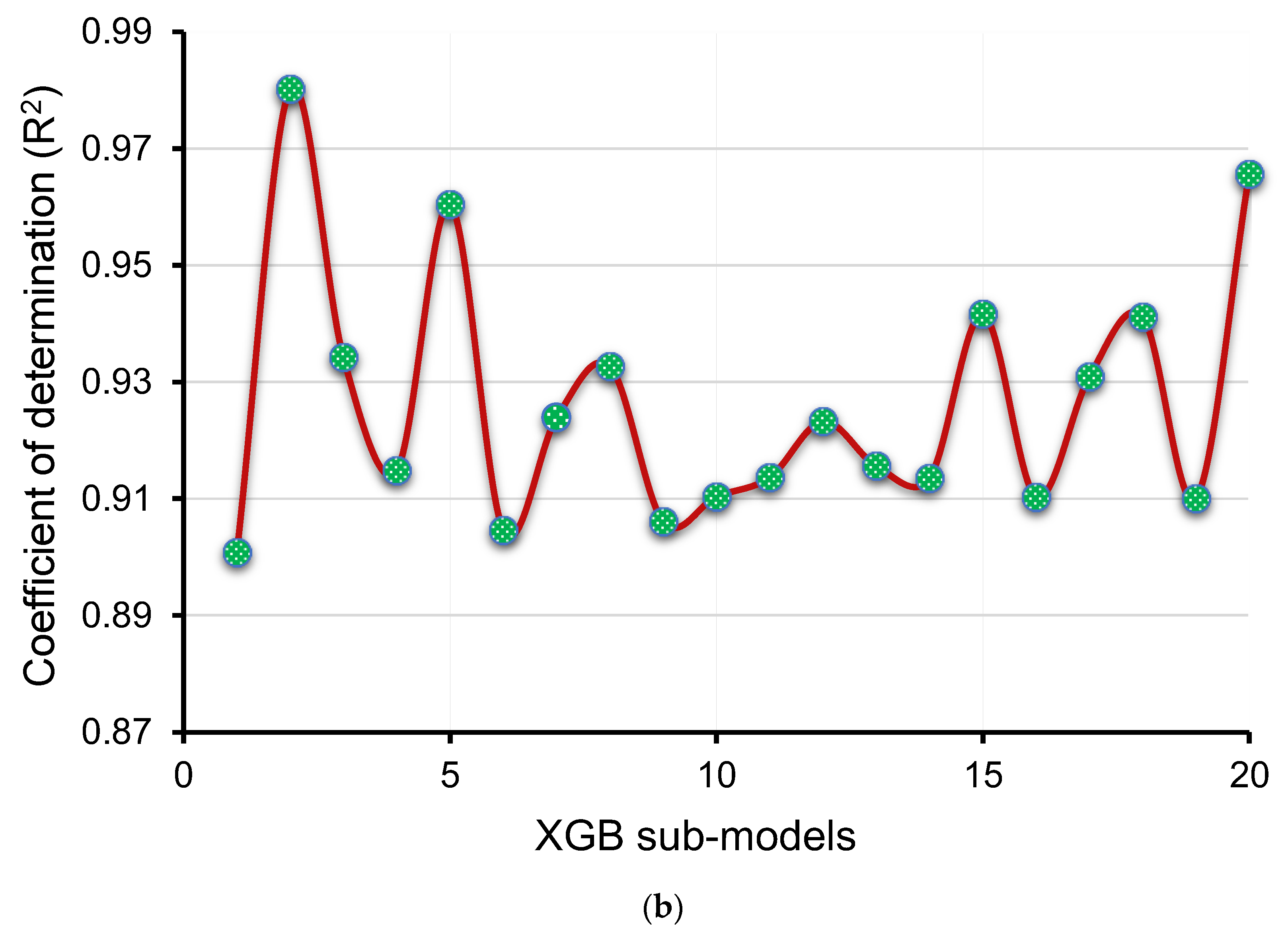
3.3. Extreme Gradient Boosting Model
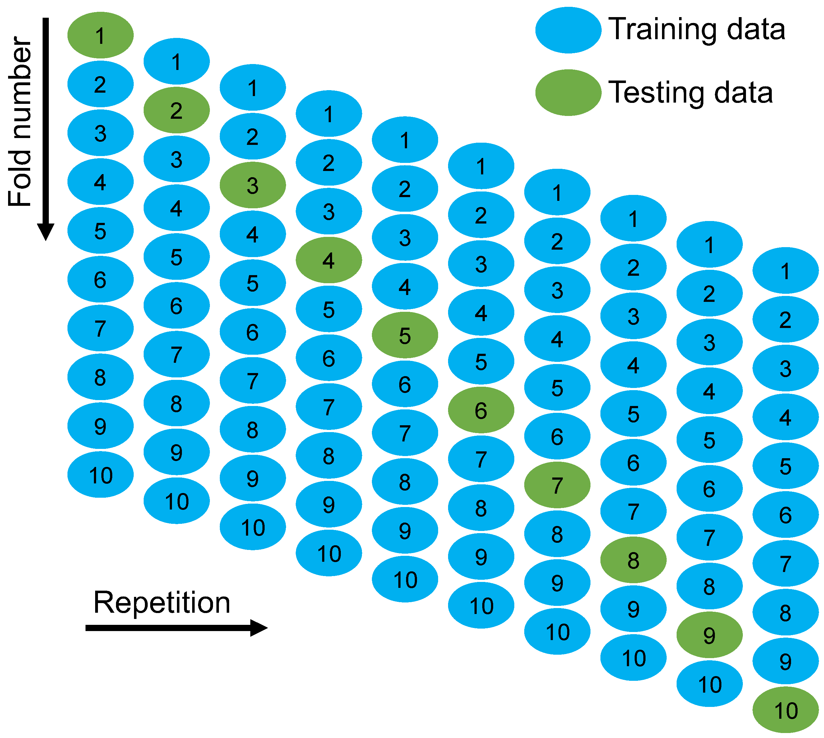
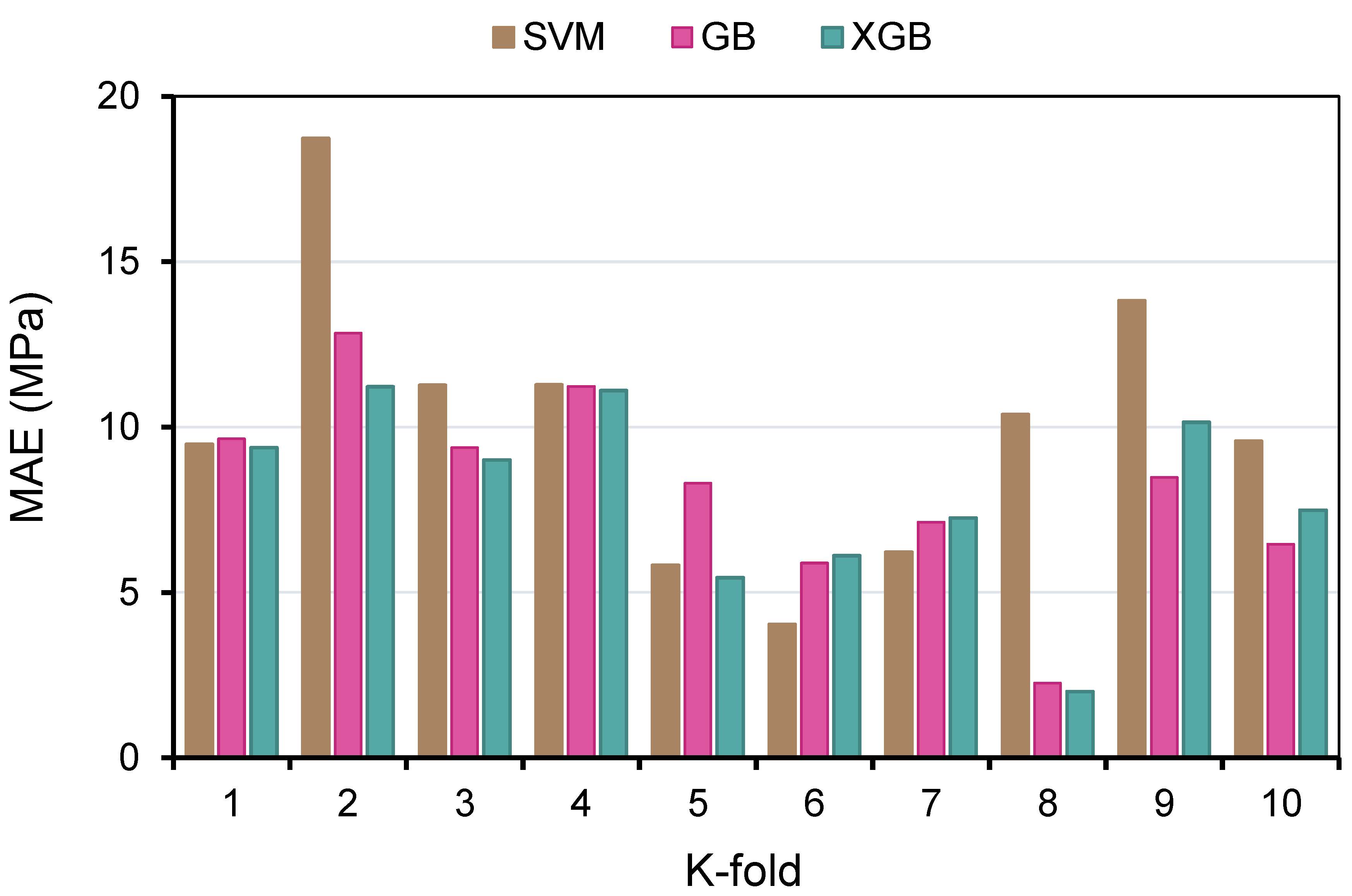
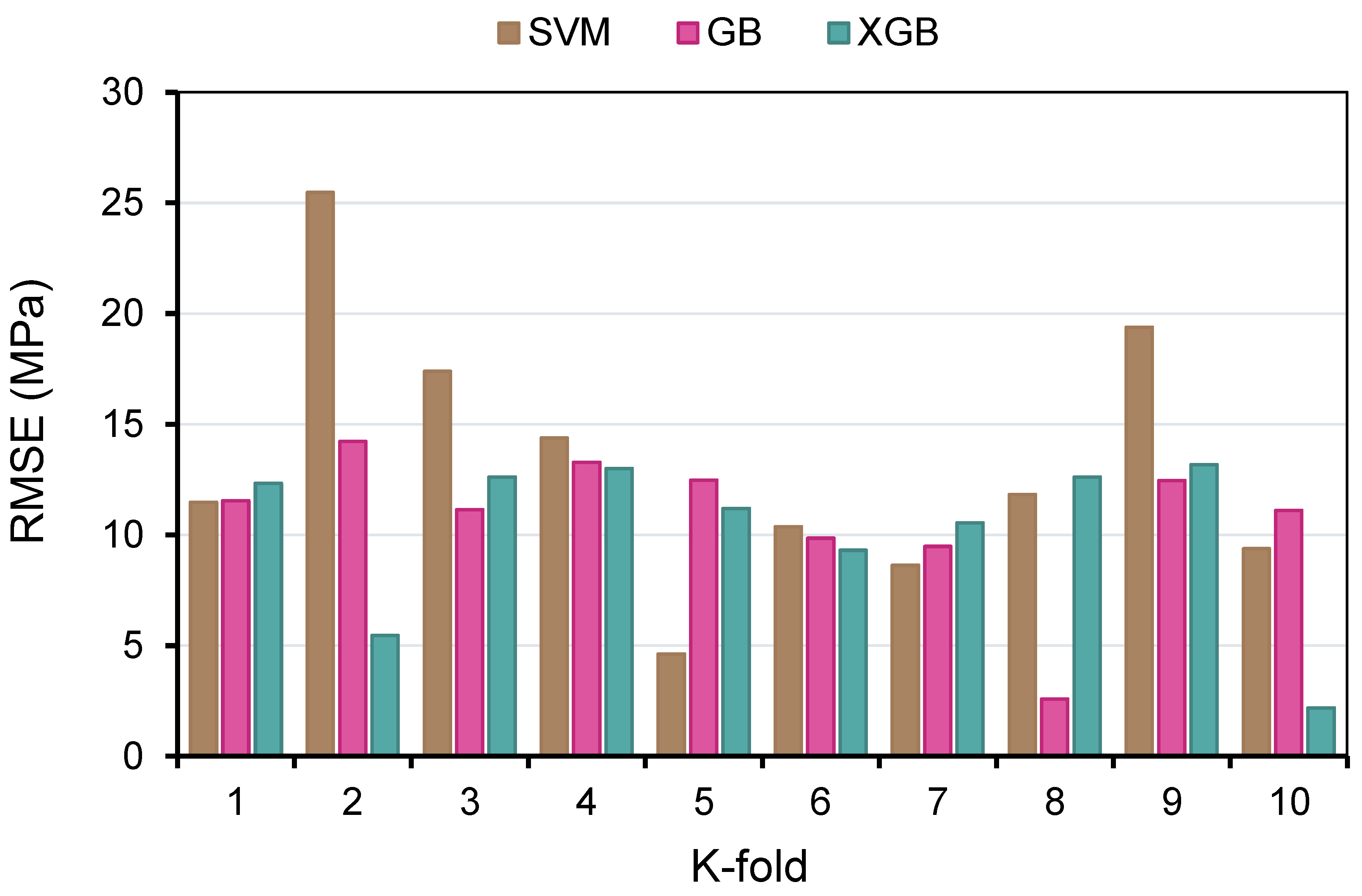
4. Models’ Validation
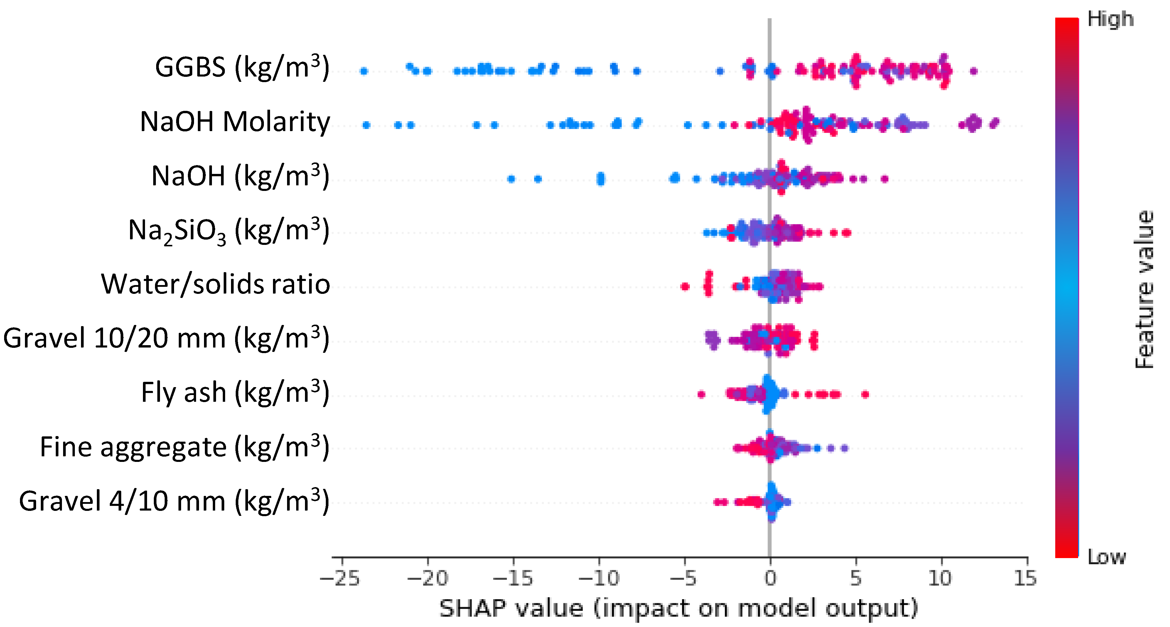
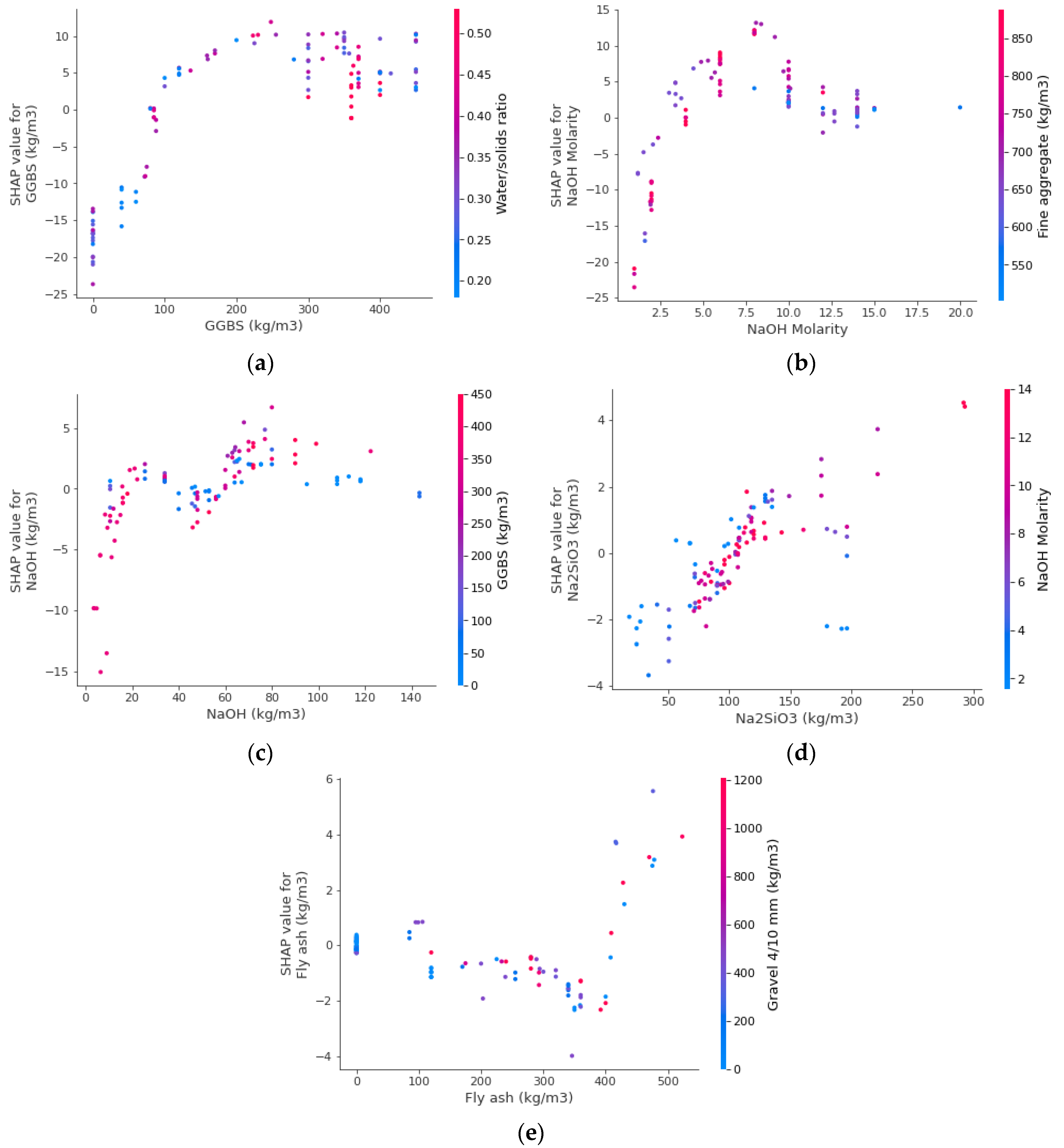
5. Influence of Input Parameters
6. Discussion
7. Conclusions
- Ensemble ML methods fared better at predicting the CS of GPCs than individual machine learning techniques, with the XGB model doing the best. For the XGB, GB, and SVM models, the coefficients of determination (R2) were 0.98, 0.97, and 0.93, respectively. All the employed techniques yielded results within a satisfactory limit and with little deviation from the experimental findings;
- These error readings also proved the best performance of the XGB method in forecasting the CS of GPC;
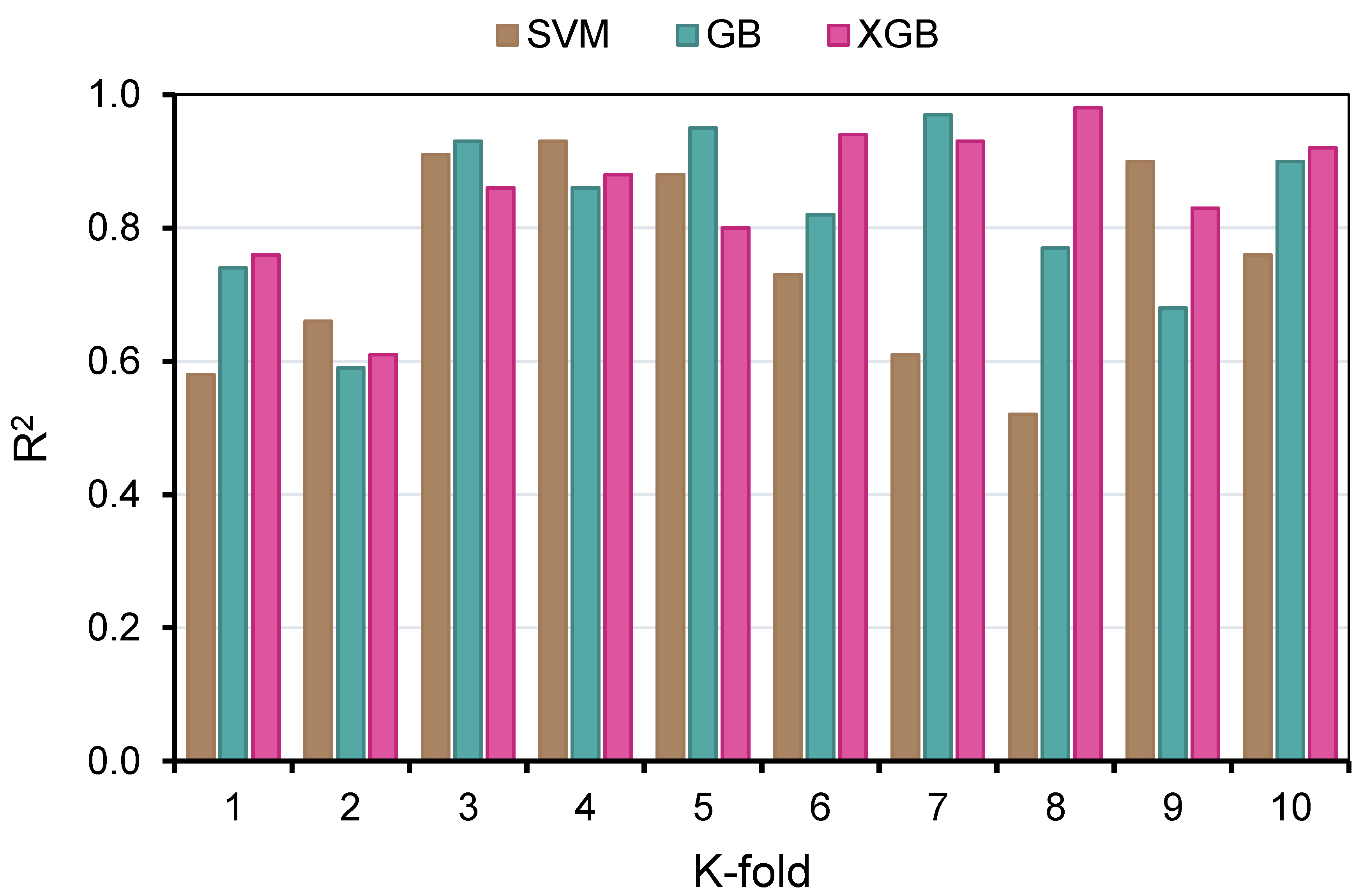
- Statistical tests and k-fold analysis validated the performance of the employed models. The smaller errors and greater R2 resulting from k-fold analysis suggested the higher precision of the ML model. These analyses indicated that the XGB model outperformed the other investigated models;
- Based on the results of the SHAP analysis, GGBS was considered to be a more influential input feature, showing a larger positive association between this characteristic and GPC’s CS;
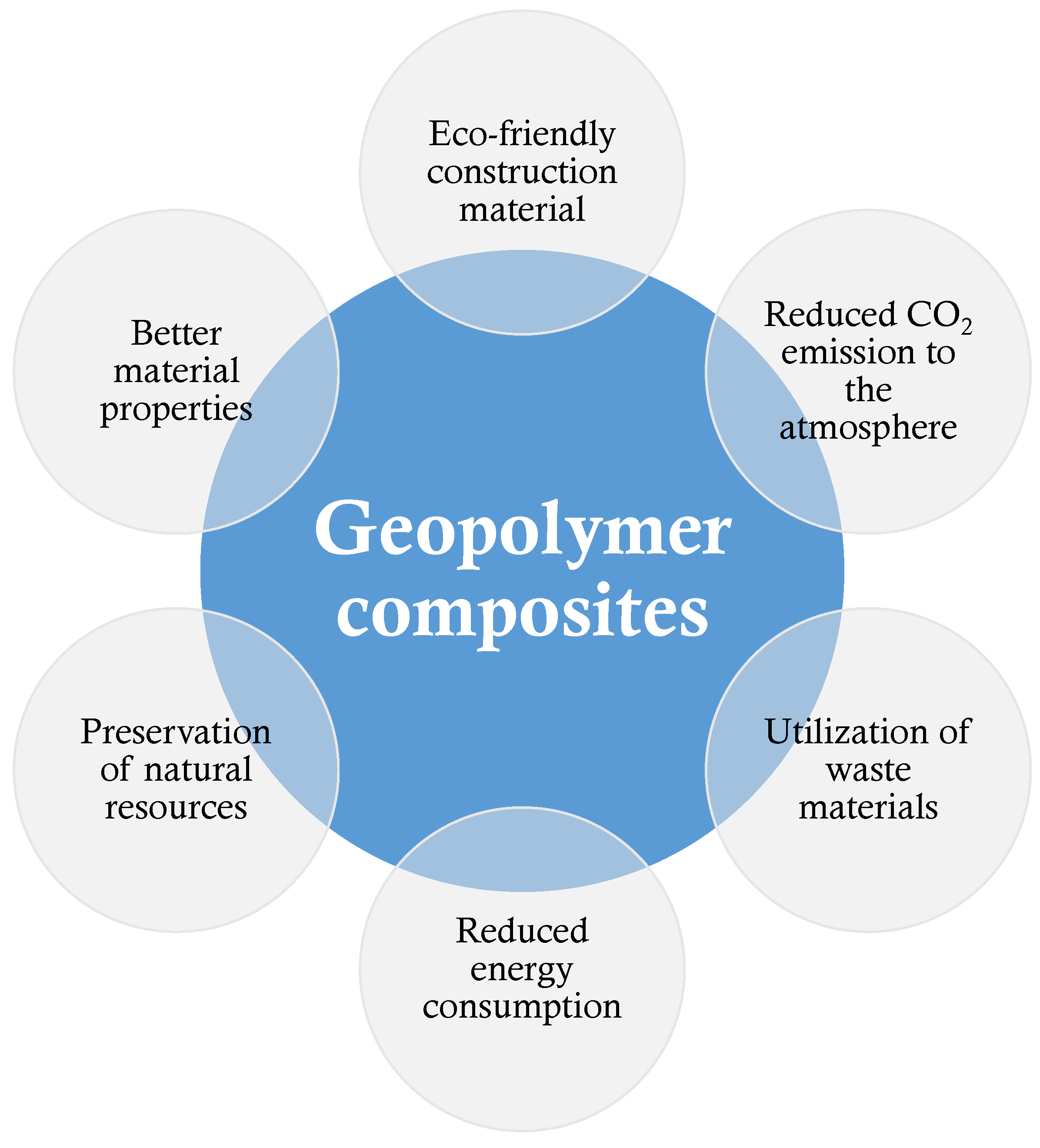
- This nature of research will help the construction industry by facilitating the development of fast and cost-efficient methods for forecasting material characteristics. Moreover, by supporting eco-friendly construction, these initiatives will hasten the acceptance and application of GPC in the building sector.
Supplementary Materials
Author Contributions
Funding
Institutional Review Board Statement
Informed Consent Statement
Data Availability Statement
Acknowledgments
Conflicts of Interest
References
- Chen, Y.; Liu, P.; Sha, F.; Yu, Z.; He, S.; Xu, W.; Lv, M. Effects of Type and Content of Fibers, Water-to-Cement Ratio, and Cementitious Materials on the Shrinkage and Creep of Ultra-High Performance Concrete. Polymers 2022, 14, 1956. [Google Scholar] [CrossRef] [PubMed]
- Khan, M.; Cao, M.; Xie, C.; Ali, M. Effectiveness of hybrid steel-basalt fiber reinforced concrete under compression. Case Stud. Constr. Mater. 2022, 16, e00941. [Google Scholar] [CrossRef]
- Khan, M.; Cao, M.; Hussain, A.; Chu, S.H. Effect of silica-fume content on performance of CaCO3 whisker and basalt fiber at matrix interface in cement-based composites. Constr. Build. Mater. 2021, 300, 124046. [Google Scholar] [CrossRef]
- Yang, H.; Liu, L.; Yang, W.; Liu, H.; Ahmad, W.; Ahmad, A.; Aslam, F.; Joyklad, P. A comprehensive overview of geopolymer composites: A bibliometric analysis and literature review. Case Stud. Constr. Mater. 2022, 16, e00830. [Google Scholar] [CrossRef]
- Khan, M.; Cao, M.; Chaopeng, X.; Ali, M. Experimental and analytical study of hybrid fiber reinforced concrete prepared with basalt fiber under high temperature. Fire Mater. 2022, 46, 205–226. [Google Scholar] [CrossRef]
- Khan, M.; Cao, M.; Ai, H.; Hussain, A. Basalt Fibers in Modified Whisker Reinforced Cementitious Composites. Period. Polytech. Civ. Eng. 2022, 66, 344–354. [Google Scholar] [CrossRef]
- Biricik, H.; Kırgız, M.S.; De Sousa Galdino, A.G.; Kenai, S.; Mirza, J.; Kinuthia, J.; Ashteyat, A.; Khitab, A.; Khatib, J. Activation of slag through a combination of NaOH/NaS alkali for transforming it into geopolymer slag binder mortar–assessment the effects of two different Blaine fines and three different curing conditions. J. Mater. Res. Technol. 2021, 14, 1569–1584. [Google Scholar] [CrossRef]
- Mahmood, A.; Noman, M.T.; Pechočiaková, M.; Amor, N.; Petrů, M.; Abdelkader, M.; Militký, J.; Sozcu, S.; Hassan, S.Z. Geopolymers and Fiber-Reinforced Concrete Composites in Civil Engineering. Polymers 2021, 13, 2099. [Google Scholar] [CrossRef]
- Farooq, F.; Jin, X.; Javed, M.F.; Akbar, A.; Shah, M.I.; Aslam, F.; Alyousef, R. Geopolymer concrete as sustainable material: A state of the art review. Constr. Build. Mater. 2021, 306, 124762. [Google Scholar] [CrossRef]
- Salas, D.A.; Ramirez, A.D.; Rodríguez, C.R.; Petroche, D.M.; Boero, A.J.; Duque-Rivera, J. Environmental impacts, life cycle assessment and potential improvement measures for cement production: A literature review. J. Clean. Prod. 2016, 113, 114–122. [Google Scholar] [CrossRef]
- Ahmed, M.; Bashar, I.; Alam, S.T.; Wasi, A.I.; Jerin, I.; Khatun, S.; Rahman, M. An overview of Asian cement industry: Environmental impacts, research methodologies and mitigation measures. Sustain. Prod. Consum. 2021, 28, 1018–1039. [Google Scholar] [CrossRef]
- Miller, S.A.; Myers, R.J. Environmental impacts of alternative cement binders. Environ. Sci. Technol. 2019, 54, 677–686. [Google Scholar] [CrossRef] [PubMed]
- Tariq, H.; Siddique, R.M.; Shah, S.A.; Azab, M.; Attiq Ur, R.; Qadeer, R.; Ullah, M.K.; Iqbal, F. Mechanical Performance of Polymeric ARGF-Based Fly Ash-Concrete Composites: A Study for Eco-Friendly Circular Economy Application. Polymers 2022, 14, 1774. [Google Scholar] [CrossRef] [PubMed]
- Alhazmi, H.; Shah, S.A.; Anwar, M.K.; Raza, A.; Ullah, M.K.; Iqbal, F. Utilization of Polymer Concrete Composites for a Circular Economy: A Comparative Review for Assessment of Recycling and Waste Utilization. Polymers 2021, 13, 2135. [Google Scholar] [CrossRef] [PubMed]
- Khan, M.; Ali, M. Improvement in concrete behavior with fly ash, silica-fume and coconut fibres. Constr. Build. Mater. 2019, 203, 174–187. [Google Scholar] [CrossRef]
- Khan, M.; Rehman, A.; Ali, M. Efficiency of silica-fume content in plain and natural fiber reinforced concrete for concrete road. Constr. Build. Mater. 2020, 244, 118382. [Google Scholar] [CrossRef]
- Ahmad, W.; Ahmad, A.; Ostrowski, K.A.; Aslam, F.; Joyklad, P.; Zajdel, P. Application of Advanced Machine Learning Approaches to Predict the Compressive Strength of Concrete Containing Supplementary Cementitious Materials. Materials 2021, 14, 5762. [Google Scholar] [CrossRef]
- Ahmad, W.; Ahmad, A.; Ostrowski, K.A.; Aslam, F.; Joyklad, P.; Zajdel, P. Sustainable approach of using sugarcane bagasse ash in cement-based composites: A systematic review. Case Stud. Constr. Mater. 2021, 15, e00698. [Google Scholar] [CrossRef]
- Juenger, M.C.G.; Snellings, R.; Bernal, S.A. Supplementary cementitious materials: New sources, characterization, and performance insights. Cem. Concr. Res. 2019, 122, 257–273. [Google Scholar] [CrossRef]
- Miller, S.A. Supplementary cementitious materials to mitigate greenhouse gas emissions from concrete: Can there be too much of a good thing? J. Clean. Prod. 2018, 178, 587–598. [Google Scholar] [CrossRef]
- Snoeck, D.; Jensen, O.M.; De Belie, N. The influence of superabsorbent polymers on the autogenous shrinkage properties of cement pastes with supplementary cementitious materials. Cem. Concr. Res. 2015, 74, 59–67. [Google Scholar] [CrossRef]
- Fares, G.; Al-Zaid, R.Z.; Fauzi, A.; Alhozaimy, A.M.; Al-Negheimish, A.I.; Khan, M.I. Performance of optimized electric arc furnace dust-based cementitious matrix compared to conventional supplementary cementitious materials. Constr. Build. Mater. 2016, 112, 210–221. [Google Scholar] [CrossRef]
- Thomas, B.S.; Yang, J.; Bahurudeen, A.; Abdalla, J.A.; Hawileh, R.A.; Hamada, H.M.; Nazar, S.; Jittin, V.; Ashish, D.K. Sugarcane bagasse ash as supplementary cementitious material in concrete—A review. Mater. Today Sustain. 2021, 15, 100086. [Google Scholar] [CrossRef]
- Li, G.; Zhou, C.; Ahmad, W.; Usanova, K.I.; Karelina, M.; Mohamed, A.M.; Khallaf, R. Fly Ash Application as Supplementary Cementitious Material: A Review. Materials 2022, 15, 2664. [Google Scholar] [CrossRef] [PubMed]
- Hefni, Y.; Abd El Zaher, Y.; Wahab, M.A. Influence of activation of fly ash on the mechanical properties of concrete. Constr. Build. Mater. 2018, 172, 728–734. [Google Scholar] [CrossRef]
- Viet, D.B.; Chan, W.-P.; Phua, Z.-H.; Ebrahimi, A.; Abbas, A.; Lisak, G. The use of fly ashes from waste-to-energy processes as mineral CO2 sequesters and supplementary cementitious materials. J. Hazard. Mater. 2020, 398, 122906. [Google Scholar] [CrossRef]
- Zaghloul, M.M.Y.; Mohamed, Y.S.; El-Gamal, H.J. Fatigue and tensile behaviors of fiber-reinforced thermosetting composites embedded with nanoparticles. J. Compos. Mater. 2019, 53, 709–718. [Google Scholar] [CrossRef]
- Fuseini, M.; Zaghloul, M.M.Y.; Elkady, M.F.; El-Shazly, A.H.J. Evaluation of synthesized polyaniline nanofibres as corrosion protection film coating on copper substrate by electrophoretic deposition. J. Mater. Sci. 2022, 57, 6085–6101. [Google Scholar] [CrossRef]
- Zaghloul, M.Y.M.; Zaghloul, M.M.Y.; Zaghloul, M.M.Y. Developments in polyester composite materials–An in-depth review on natural fibres and nano fillers. Compos. Struct. 2021, 278, 114698. [Google Scholar] [CrossRef]
- Han, X.; Yang, J.; Feng, J.; Zhou, C.; Wang, X. Research on hydration mechanism of ultrafine fly ash and cement composite. Constr. Build. Mater. 2019, 227, 116697. [Google Scholar] [CrossRef]
- Wu, M.; Sui, S.; Zhang, Y.; Jia, Y.; She, W.; Liu, Z.; Yang, Y. Analyzing the filler and activity effect of fly ash and slag on the early hydration of blended cement based on calorimetric test. Constr. Build. Mater. 2021, 276, 122201. [Google Scholar] [CrossRef]
- Zhou, Z.; Sofi, M.; Liu, J.; Li, S.; Zhong, A.; Mendis, P. Nano-CSH modified high volume fly ash concrete: Early-age properties and environmental impact analysis. J. Clean. Prod. 2021, 286, 124924. [Google Scholar] [CrossRef]
- Provis, J.L. Alkali-activated materials. Cem. Concr. Res. 2018, 114, 40–48. [Google Scholar] [CrossRef]
- Pacheco-Torgal, F.; Castro-Gomes, J.; Jalali, S. Alkali-activated binders: A review: Part 1. Historical background, terminology, reaction mechanisms and hydration products. Constr. Build. Mater. 2008, 22, 1305–1314. [Google Scholar] [CrossRef] [Green Version]
- Marvila, M.T.; Azevedo, A.R.G.d.; Vieira, C.M.F. Reaction mechanisms of alkali-activated materials. Rev. IBRACON Estrut. Mater. 2021, 14, e14309. [Google Scholar] [CrossRef]
- Mohamed, O.A. A review of durability and strength characteristics of alkali-activated slag concrete. Materials 2019, 12, 1198. [Google Scholar] [CrossRef] [Green Version]
- Peng, Y.; Unluer, C. Analyzing the mechanical performance of fly ash-based geopolymer concrete with different machine learning techniques. Constr. Build. Mater. 2022, 316, 125785. [Google Scholar] [CrossRef]
- Mohamed, O.A.; Al Khattab, R. Fresh Properties and Sulfuric Acid Resistance of Sustainable Mortar Using Alkali-Activated GGBS/Fly Ash Binder. Polymers 2022, 14, 591. [Google Scholar] [CrossRef] [PubMed]
- Algaifi, H.A.; Mustafa Mohamed, A.; Alsuhaibani, E.; Shahidan, S.; Alrshoudi, F.; Huseien, G.F.; Bakar, S.A. Optimisation of GBFS, Fly Ash, and Nano-Silica Contents in Alkali-Activated Mortars. Polymers 2021, 13, 2750. [Google Scholar] [CrossRef]
- Ahmad, A.; Ahmad, W.; Aslam, F.; Joyklad, P. Compressive strength prediction of fly ash-based geopolymer concrete via advanced machine learning techniques. Case Stud. Constr. Mater. 2022, 16, e00840. [Google Scholar] [CrossRef]
- Ahmad, A.; Ahmad, W.; Chaiyasarn, K.; Ostrowski, K.A.; Aslam, F.; Zajdel, P.; Joyklad, P. Prediction of Geopolymer Concrete Compressive Strength Using Novel Machine Learning Algorithms. Polymers 2021, 13, 3389. [Google Scholar] [CrossRef] [PubMed]
- Wong, L.S. Durability Performance of Geopolymer Concrete: A Review. Polymers 2022, 14, 868. [Google Scholar] [CrossRef] [PubMed]
- Okoye, F.N. Geopolymer binder: A veritable alternative to Portland cement. Mater. Today Proc. 2017, 4, 5599–5604. [Google Scholar] [CrossRef]
- Ramujee, K.; Potharaju, M. Mechanical properties of geopolymer concrete composites. Mater. Today Proc. 2017, 4, 2937–2945. [Google Scholar] [CrossRef]
- Komnitsas, K.; Zaharaki, D. Geopolymerisation: A review and prospects for the minerals industry. Miner. Eng. 2007, 20, 1261–1277. [Google Scholar] [CrossRef]
- Awoyera, P.O. Nonlinear finite element analysis of steel fibre-reinforced concrete beam under static loading. J. Eng. Sci. Technol. 2016, 11, 1669–1677. [Google Scholar]
- Cao, M.; Mao, Y.; Khan, M.; Si, W.; Shen, S. Different testing methods for assessing the synthetic fiber distribution in cement-based composites. Constr. Build. Mater. 2018, 184, 128–142. [Google Scholar] [CrossRef]
- Sadrmomtazi, A.; Sobhani, J.; Mirgozar, M.A. Modeling compressive strength of EPS lightweight concrete using regression, neural network and ANFIS. Constr. Build. Mater. 2013, 42, 205–216. [Google Scholar] [CrossRef]
- Ilyas, I.; Zafar, A.; Afzal, M.T.; Javed, M.F.; Alrowais, R.; Althoey, F.; Mohamed, A.M.; Mohamed, A.; Vatin, N.I. Advanced Machine Learning Modeling Approach for Prediction of Compressive Strength of FRP Confined Concrete Using Multiphysics Genetic Expression Programming. Polymers 2022, 14, 1789. [Google Scholar] [CrossRef]
- Nafees, A.; Khan, S.; Javed, M.F.; Alrowais, R.; Mohamed, A.M.; Mohamed, A.; Vatin, N.I. Forecasting the Mechanical Properties of Plastic Concrete Employing Experimental Data Using Machine Learning Algorithms: DT, MLPNN, SVM, and RF. Polymers 2022, 14, 1583. [Google Scholar] [CrossRef]
- Nafees, A.; Amin, M.N.; Khan, K.; Nazir, K.; Ali, M.; Javed, M.F.; Aslam, F.; Musarat, M.A.; Vatin, N.I. Modeling of Mechanical Properties of Silica Fume-Based Green Concrete Using Machine Learning Techniques. Polymers 2022, 14, 30. [Google Scholar] [CrossRef] [PubMed]
- Khan, K.; Ahmad, A.; Amin, M.N.; Ahmad, W.; Nazar, S.; Arab, A.M.A. Comparative Study of Experimental and Modeling of Fly Ash-Based Concrete. Materials 2022, 15, 3762. [Google Scholar] [CrossRef] [PubMed]
- Nafees, A.; Javed, M.F.; Khan, S.; Nazir, K.; Farooq, F.; Aslam, F.; Musarat, M.A.; Vatin, N.I. Predictive Modeling of Mechanical Properties of Silica Fume-Based Green Concrete Using Artificial Intelligence Approaches: MLPNN, ANFIS, and GEP. Materials 2021, 14, 7531. [Google Scholar] [CrossRef] [PubMed]
- Öztaş, A.; Pala, M.; Özbay, E.A.; Kanca, E.; Caglar, N.; Bhatti, M.A. Predicting the compressive strength and slump of high strength concrete using neural network. Constr. Build. Mater. 2006, 20, 769–775. [Google Scholar] [CrossRef]
- Sarıdemir, M. Predicting the compressive strength of mortars containing metakaolin by artificial neural networks and fuzzy logic. Adv. Eng. Softw. 2009, 40, 920–927. [Google Scholar] [CrossRef]
- Ni, H.-G.; Wang, J.-Z. Prediction of compressive strength of concrete by neural networks. Cem. Concr. Res. 2000, 30, 1245–1250. [Google Scholar] [CrossRef]
- Sobhani, J.; Najimi, M.; Pourkhorshidi, A.R.; Parhizkar, T. Prediction of the compressive strength of no-slump concrete: A comparative study of regression, neural network and ANFIS models. Constr. Build. Mater. 2010, 24, 709–718. [Google Scholar] [CrossRef]
- Awoyera, P.O.; Kirgiz, M.S.; Viloria, A.; Ovallos-Gazabon, D. Estimating strength properties of geopolymer self-compacting concrete using machine learning techniques. J. Mater. Res. Technol. 2020, 9, 9016–9028. [Google Scholar] [CrossRef]
- Shafabakhsh, G.H.; Ani, O.J.; Talebsafa, M. Artificial neural network modeling (ANN) for predicting rutting performance of nano-modified hot-mix asphalt mixtures containing steel slag aggregates. Constr. Build. Mater. 2015, 85, 136–143. [Google Scholar] [CrossRef]
- Hodhod, O.A.; Ahmed, H.I. Modeling the corrosion initiation time of slag concrete using the artificial neural network. HBRC J. 2014, 10, 231–234. [Google Scholar] [CrossRef] [Green Version]
- Carmichael, R.P. Relationships between Young’s Modulus, Compressive Strength, Poisson’s Ratio, and Time for Early Age Concrete; Swarthmore College: Swarthmore, PA, USA, 2009; Volume 123, pp. 317–326. [Google Scholar]
- Bal, L.; Buyle-Bodin, F. Artificial neural network for predicting drying shrinkage of concrete. Constr. Build. Mater. 2013, 38, 248–254. [Google Scholar] [CrossRef]
- Chou, J.-S.; Tsai, C.-F.; Pham, A.-D.; Lu, Y.-H. Machine learning in concrete strength simulations: Multi-nation data analytics. Constr. Build. Mater. 2014, 73, 771–780. [Google Scholar] [CrossRef]
- Young, B.A.; Hall, A.; Pilon, L.; Gupta, P.; Sant, G. Can the compressive strength of concrete be estimated from knowledge of the mixture proportions?: New insights from statistical analysis and machine learning methods. Cem. Concr. Res. 2019, 115, 379–388. [Google Scholar] [CrossRef]
- Akande, K.O.; Owolabi, T.O.; Twaha, S.; Olatunji, S.O. Performance comparison of SVM and ANN in predicting compressive strength of concrete. IOSR J. Comput. Eng. 2014, 16, 88–94. [Google Scholar] [CrossRef]
- Behnood, A.; Behnood, V.; Gharehveran, M.M.; Alyamac, K.E. Prediction of the compressive strength of normal and high-performance concretes using M5P model tree algorithm. Constr. Build. Mater. 2017, 142, 199–207. [Google Scholar] [CrossRef]
- Duan, Z.-H.; Kou, S.-C.; Poon, C.-S. Prediction of compressive strength of recycled aggregate concrete using artificial neural networks. Constr. Build. Mater. 2013, 40, 1200–1206. [Google Scholar] [CrossRef]
- De Melo, V.V.; Banzhaf, W. Improving the prediction of material properties of concrete using Kaizen Programming with Simulated Annealing. Neurocomputing 2017, 246, 25–44. [Google Scholar] [CrossRef]
- Yeh, I.C.; Lien, L.-C. Knowledge discovery of concrete material using genetic operation trees. Expert Syst. Appl. 2009, 36, 5807–5812. [Google Scholar] [CrossRef]
- Chaabene, W.B.; Flah, M.; Nehdi, M.L. Machine learning prediction of mechanical properties of concrete: Critical review. Constr. Build. Mater. 2020, 260, 119889. [Google Scholar] [CrossRef]
- Dao, D.V.; Trinh, S.H.; Ly, H.-B.; Pham, B.T. Prediction of compressive strength of geopolymer concrete using entirely steel slag aggregates: Novel hybrid artificial intelligence approaches. Appl. Sci. 2019, 9, 1113. [Google Scholar] [CrossRef] [Green Version]
- Dao, D.V.; Ly, H.-B.; Trinh, S.H.; Le, T.-T.; Pham, B.T. Artificial intelligence approaches for prediction of compressive strength of geopolymer concrete. Materials 2019, 12, 983. [Google Scholar] [CrossRef] [PubMed] [Green Version]
- Sufian, M.; Ullah, S.; Ostrowski, K.A.; Ahmad, A.; Zia, A.; Śliwa-Wieczorek, K.; Siddiq, M.; Awan, A.A. An Experimental and Empirical Study on the Use of Waste Marble Powder in Construction Material. Materials 2021, 14, 3829. [Google Scholar] [CrossRef] [PubMed]
- Song, Y.-Y.; Ying, L.U. Decision tree methods: Applications for classification and prediction. Shanghai Arch. Psychiatry 2015, 27, 130. [Google Scholar] [PubMed]
- Hillebrand, E.; Medeiros, M.C. The benefits of bagging for forecast models of realized volatility. Econom. Rev. 2010, 29, 571–593. [Google Scholar] [CrossRef]
- Ling, H.; Qian, C.; Kang, W.; Liang, C.; Chen, H. Combination of Support Vector Machine and K-Fold cross validation to predict compressive strength of concrete in marine environment. Constr. Build. Mater. 2019, 206, 355–363. [Google Scholar] [CrossRef]
- Friedman, J.H. Greedy function approximation: A gradient boosting machine. Ann. Stat. 2001, 29, 1189–1232. [Google Scholar] [CrossRef]
- Dahiya, N.; Saini, B.; Chalak, H.D. Gradient boosting-based regression modelling for estimating the time period of the irregular precast concrete structural system with cross bracing. J. King Saud. Univ. Eng. Sci. 2021; in press. [Google Scholar] [CrossRef]
- Yuan, X.; Tian, Y.; Ahmad, W.; Ahmad, A.; Usanova, K.I.; Mohamed, A.M.; Khallaf, R. Machine Learning Prediction Models to Evaluate the Strength of Recycled Aggregate Concrete. Materials 2022, 15, 2823. [Google Scholar] [CrossRef]
- Alqahtani, M.; Gumaei, A.; Mathkour, H.; Maher Ben Ismail, M. A Genetic-Based Extreme Gradient Boosting Model for Detecting Intrusions in Wireless Sensor Networks. Sensors 2019, 19, 4383. [Google Scholar] [CrossRef] [Green Version]
- Ahmad, A.; Chaiyasarn, K.; Farooq, F.; Ahmad, W.; Suparp, S.; Aslam, F. Compressive Strength Prediction via Gene Expression Programming (GEP) and Artificial Neural Network (ANN) for Concrete Containing RCA. Buildings 2021, 11, 324. [Google Scholar] [CrossRef]
- Farooq, F.; Ahmed, W.; Akbar, A.; Aslam, F.; Alyousef, R. Predictive modeling for sustainable high-performance concrete from industrial wastes: A comparison and optimization of models using ensemble learners. J. Clean. Prod. 2021, 292, 126032. [Google Scholar] [CrossRef]
- Aslam, F.; Farooq, F.; Amin, M.N.; Khan, K.; Waheed, A.; Akbar, A.; Javed, M.F.; Alyousef, R.; Alabdulijabbar, H. Applications of gene expression programming for estimating compressive strength of high-strength concrete. Adv. Civ. Eng. 2020, 2020, 8850535. [Google Scholar] [CrossRef]
- Wang, Q.; Ahmad, W.; Ahmad, A.; Aslam, F.; Mohamed, A.; Vatin, N.I. Application of Soft Computing Techniques to Predict the Strength of Geopolymer Composites. Polymers 2022, 14, 1074. [Google Scholar] [CrossRef] [PubMed]
- Lundberg, S.M.; Erion, G.; Chen, H.; DeGrave, A.; Prutkin, J.M.; Nair, B.; Katz, R.; Himmelfarb, J.; Bansal, N.; Lee, S.-I. Explainable AI for trees: From local explanations to global understanding. arXiv 2019, arXiv:1905.04610. [Google Scholar] [CrossRef]
- Cao, R.; Fang, Z.; Jin, M.; Shang, Y. Application of Machine Learning Approaches to Predict the Strength Property of Geopolymer Concrete. Materials 2022, 15, 2400. [Google Scholar] [CrossRef]


| Parameter | Fine Aggregate (kg/m3) | GGBS (kg/m3) | Fly Ash (kg/m3) | NaOH Molarity | Water/Solids Ratio | Na2SiO3 (kg/m3) | NaOH (kg/m3) | Gravel Size: 4/10 mm (kg/m3) | Gravel Size: 10/20 mm (kg/m3) | CS (MPa) |
|---|---|---|---|---|---|---|---|---|---|---|
| Mean | 729.88 | 225.15 | 174.34 | 8.14 | 0.34 | 111.66 | 53.74 | 288.39 | 737.37 | 43.28 |
| Mode | 651 | 0 | 0 | 10 | 0.53 | 108 | 64 | 0 | 0 | 56.00 |
| Median | 728 | 300 | 120 | 9.2 | 0.34 | 108 | 56 | 208 | 789 | 42.10 |
| Maximum | 1360 | 450 | 523 | 20 | 0.63 | 342 | 147 | 1293.4 | 1298 | 86.08 |
| Minimum | 459 | 0 | 0 | 1 | 0 | 18 | 3.5 | 0 | 0 | 8.00 |
| Standard Deviation | 130.97 | 162.27 | 167.95 | 4.56 | 0.11 | 48.16 | 31.91 | 372.31 | 358.55 | 17.87 |
| Sum | 26,4947.79 | 81,728.05 | 63,286.04 | 2955.11 | 124.78 | 40,532.68 | 19,508.75 | 104,684.28 | 267,664.93 | 15,710.40 |
| Range | 901 | 450 | 523 | 19 | 0.63 | 324 | 143.5 | 1293.4 | 1298 | 78.08 |
| Standard Error | 6.87 | 8.52 | 8.82 | 0.24 | 0.01 | 2.53 | 1.67 | 19.54 | 18.82 | 0.94 |
| Machine Learning Model | MAE (MPa) | RMSE (MPa) |
|---|---|---|
| Support vector machine | 4.03 | 4.62 |
| Gradient boosting | 2.26 | 2.59 |
| Extreme gradient boosting | 2.01 | 2.18 |
| K-Fold | Support Vector Machine | Gradient Boosting | Extreme Gradient Boosting | ||||||
|---|---|---|---|---|---|---|---|---|---|
| MAE (MPa) | RMSE (MPa) | R2 | MAE (MPa) | RMSE (MPa) | R2 | MAE (MPa) | RMSE (MPa) | R2 | |
| 1 | 9.48 | 11.47 | 0.58 | 9.64 | 11.54 | 0.74 | 9.38 | 12.33 | 0.76 |
| 2 | 18.73 | 25.48 | 0.66 | 12.84 | 14.23 | 0.59 | 11.22 | 5.45 | 0.61 |
| 3 | 11.27 | 17.38 | 0.91 | 9.38 | 11.14 | 0.93 | 9.00 | 12.61 | 0.86 |
| 4 | 11.28 | 14.38 | 0.93 | 11.23 | 13.28 | 0.86 | 11.10 | 13.00 | 0.88 |
| 5 | 5.82 | 4.62 | 0.88 | 8.30 | 12.48 | 0.95 | 5.45 | 11.19 | 0.80 |
| 6 | 4.03 | 10.38 | 0.73 | 5.89 | 9.84 | 0.82 | 6.11 | 9.30 | 0.94 |
| 7 | 6.22 | 8.63 | 0.61 | 7.12 | 9.48 | 0.97 | 7.25 | 10.55 | 0.93 |
| 8 | 10.38 | 11.83 | 0.52 | 2.26 | 2.59 | 0.77 | 2.01 | 12.61 | 0.98 |
| 9 | 13.82 | 19.38 | 0.90 | 8.48 | 12.45 | 0.68 | 10.15 | 13.18 | 0.83 |
| 10 | 9.58 | 9.37 | 0.76 | 6.46 | 11.10 | 0.90 | 7.49 | 2.18 | 0.92 |
Publisher’s Note: MDPI stays neutral with regard to jurisdictional claims in published maps and institutional affiliations. |
© 2022 by the authors. Licensee MDPI, Basel, Switzerland. This article is an open access article distributed under the terms and conditions of the Creative Commons Attribution (CC BY) license (https://creativecommons.org/licenses/by/4.0/).
Share and Cite
Khan, K.; Ahmad, W.; Amin, M.N.; Ahmad, A.; Nazar, S.; Al-Faiad, M.A. Assessment of Artificial Intelligence Strategies to Estimate the Strength of Geopolymer Composites and Influence of Input Parameters. Polymers 2022, 14, 2509. https://doi.org/10.3390/polym14122509
Khan K, Ahmad W, Amin MN, Ahmad A, Nazar S, Al-Faiad MA. Assessment of Artificial Intelligence Strategies to Estimate the Strength of Geopolymer Composites and Influence of Input Parameters. Polymers. 2022; 14(12):2509. https://doi.org/10.3390/polym14122509
Chicago/Turabian StyleKhan, Kaffayatullah, Waqas Ahmad, Muhammad Nasir Amin, Ayaz Ahmad, Sohaib Nazar, and Majdi Adel Al-Faiad. 2022. "Assessment of Artificial Intelligence Strategies to Estimate the Strength of Geopolymer Composites and Influence of Input Parameters" Polymers 14, no. 12: 2509. https://doi.org/10.3390/polym14122509
APA StyleKhan, K., Ahmad, W., Amin, M. N., Ahmad, A., Nazar, S., & Al-Faiad, M. A. (2022). Assessment of Artificial Intelligence Strategies to Estimate the Strength of Geopolymer Composites and Influence of Input Parameters. Polymers, 14(12), 2509. https://doi.org/10.3390/polym14122509