Extensive CGMD Simulations of Atactic PS Providing Pseudo Experimental Data to Calibrate Nonlinear Inelastic Continuum Mechanical Constitutive Laws


Abstract
:
1. Introduction and Outline
2. Preparation of MD Systems
3. Model and Simulation Set Up
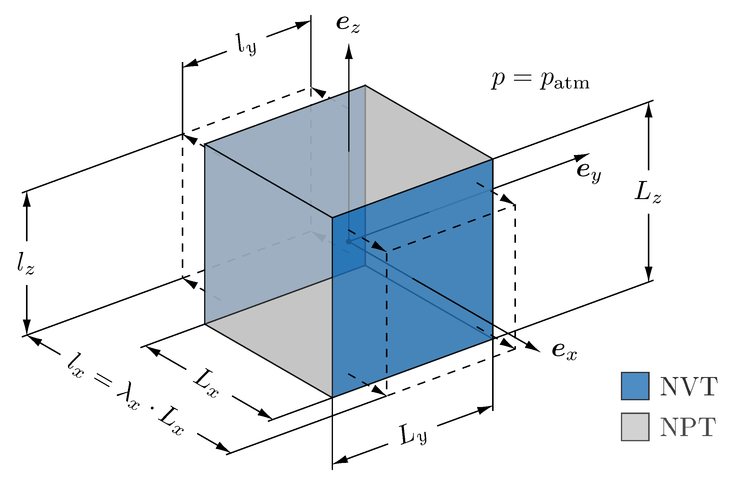
3.1. Continuum Mechanical Set Up
3.2. Molecular Dynamics Set Up
4. Uniaxial Deformation Simulations
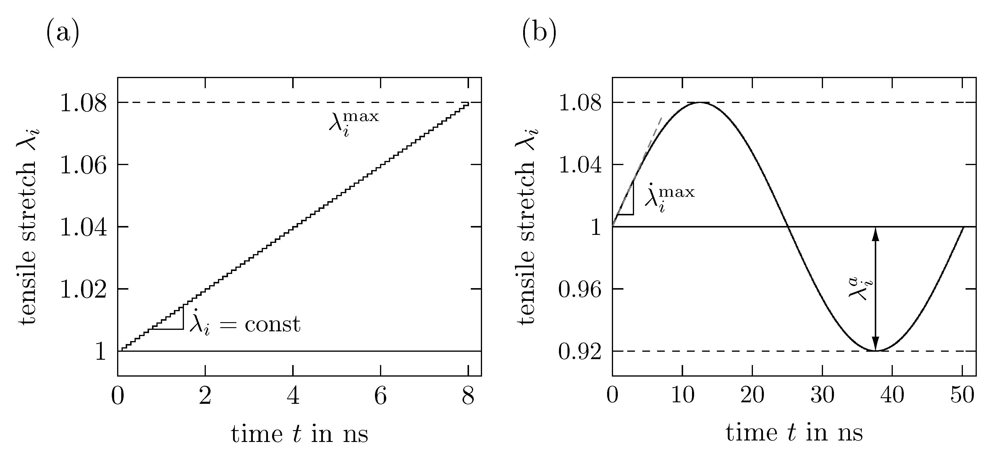
4.1. Applied Deformation
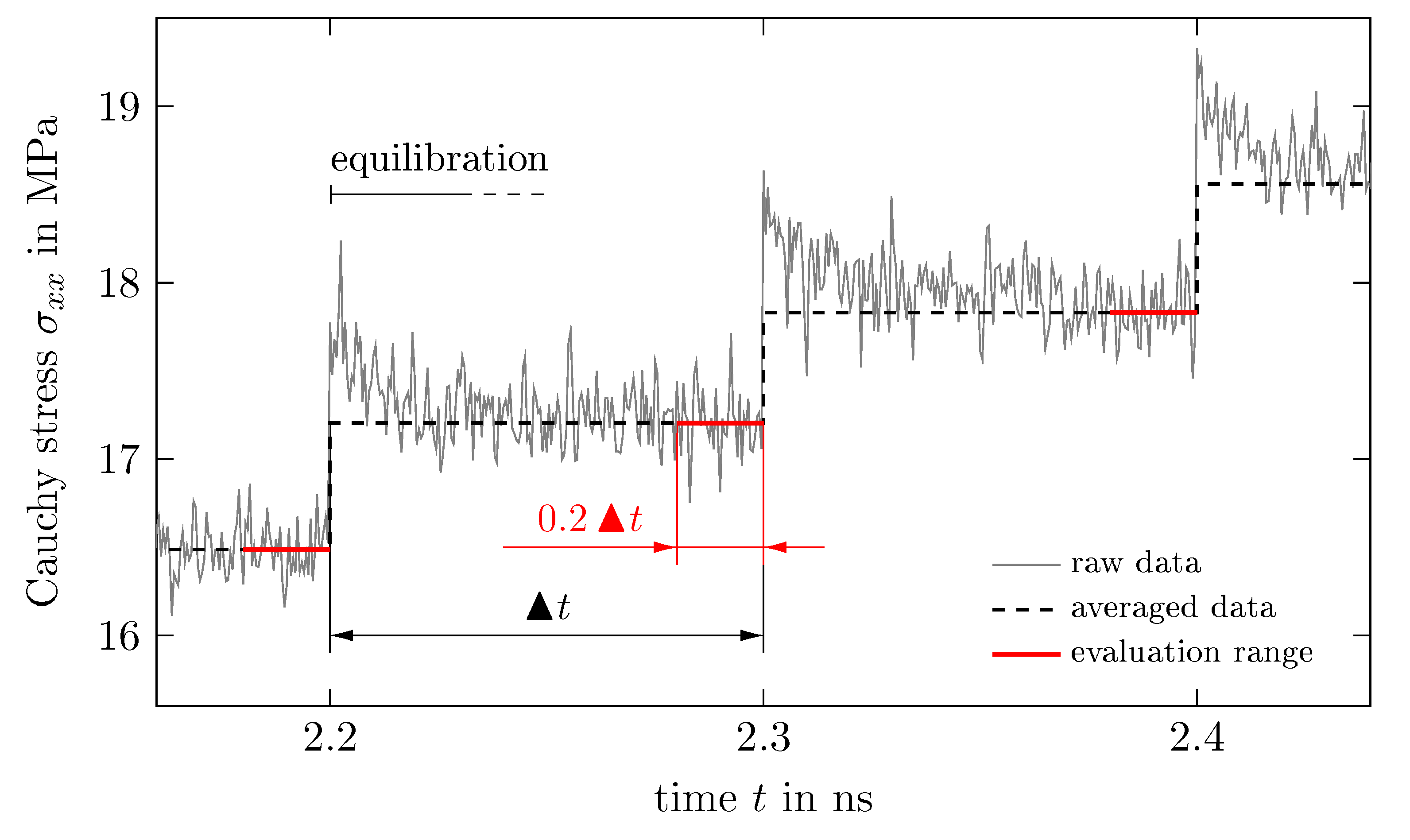
4.2. Stress Evaluation
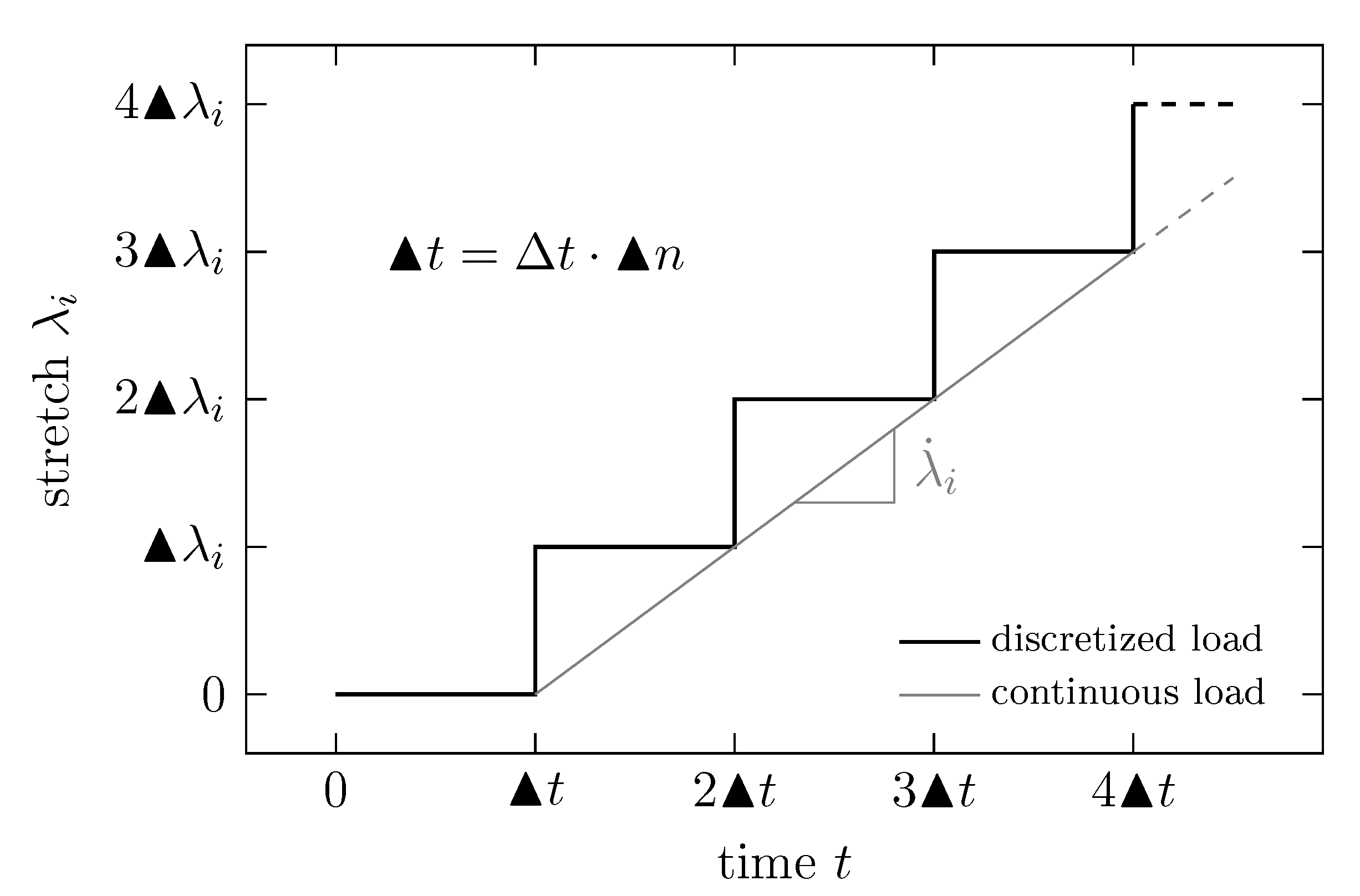
4.3. Time Discretization
5. Results
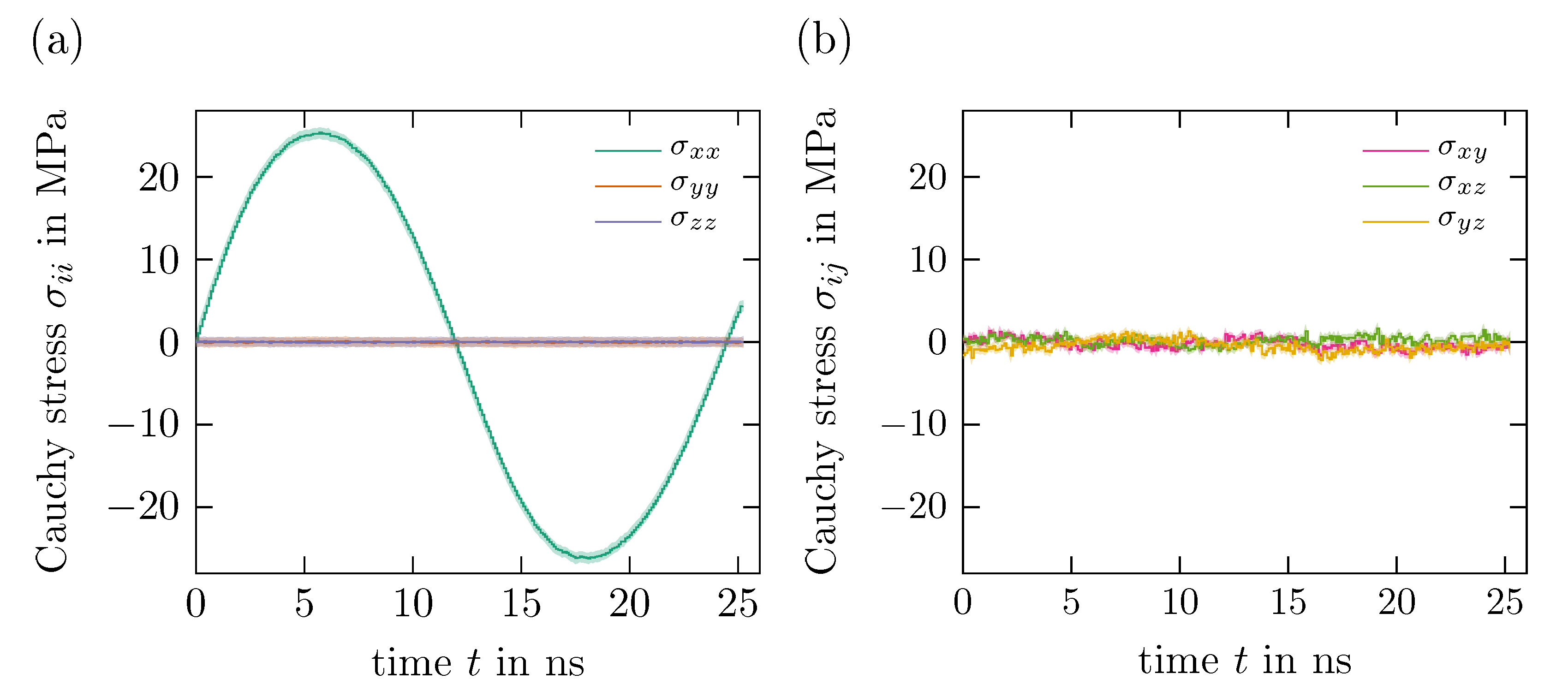
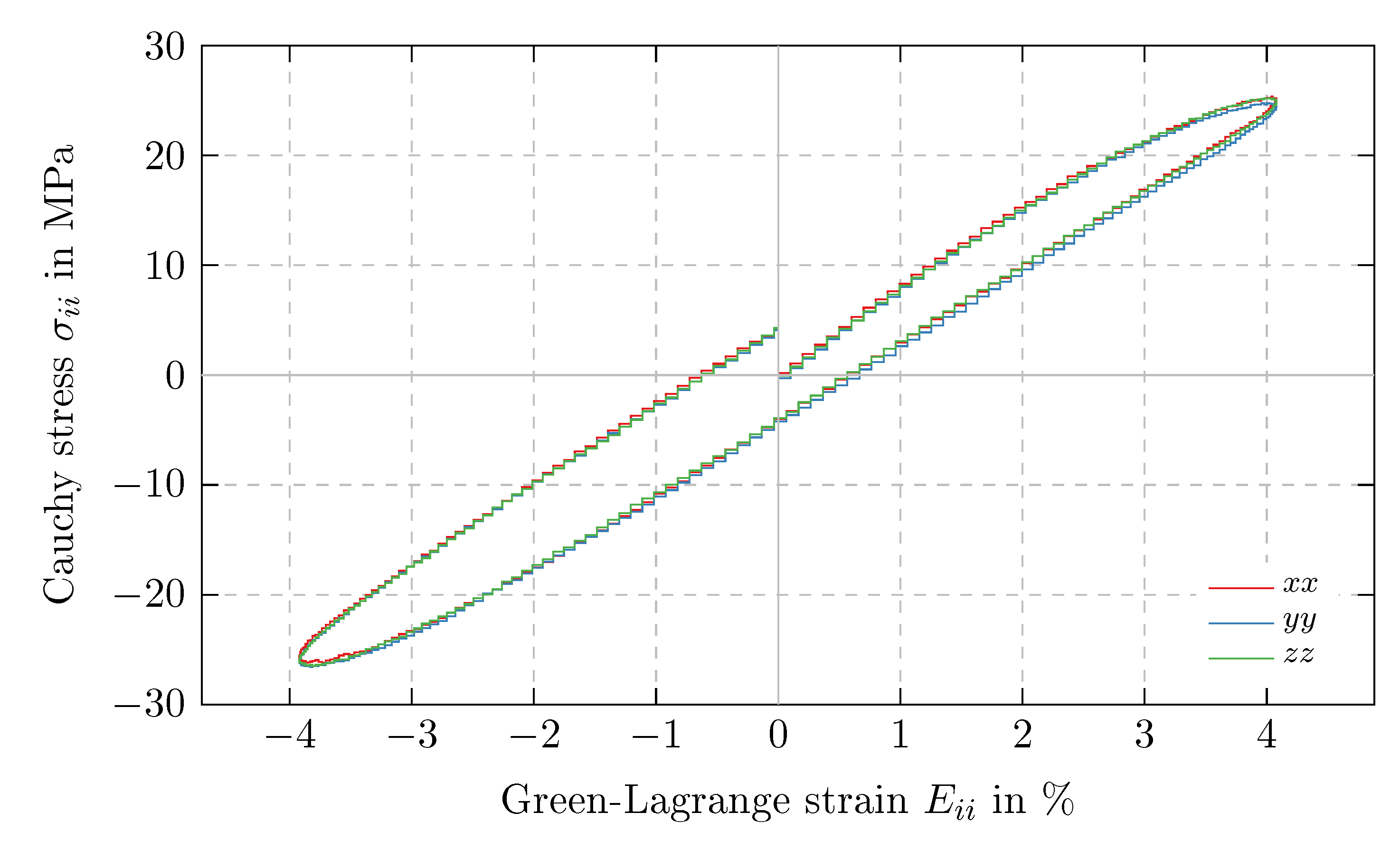
5.1. Isotropy
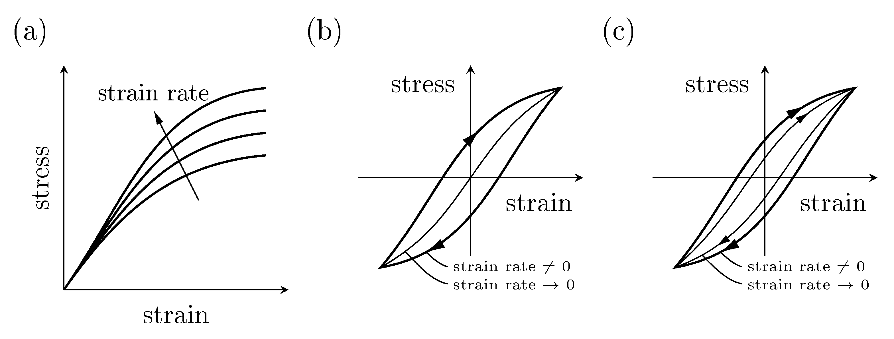
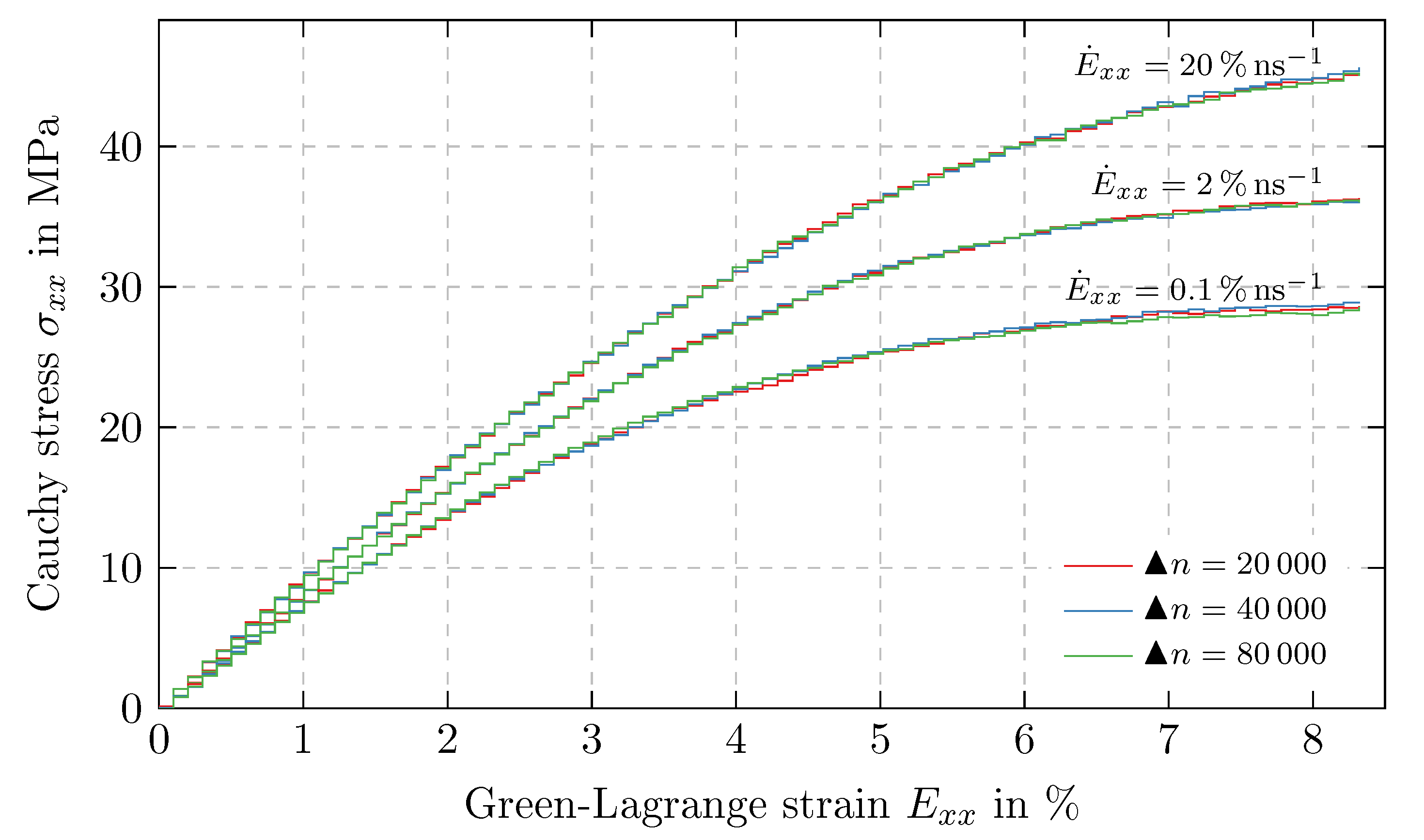
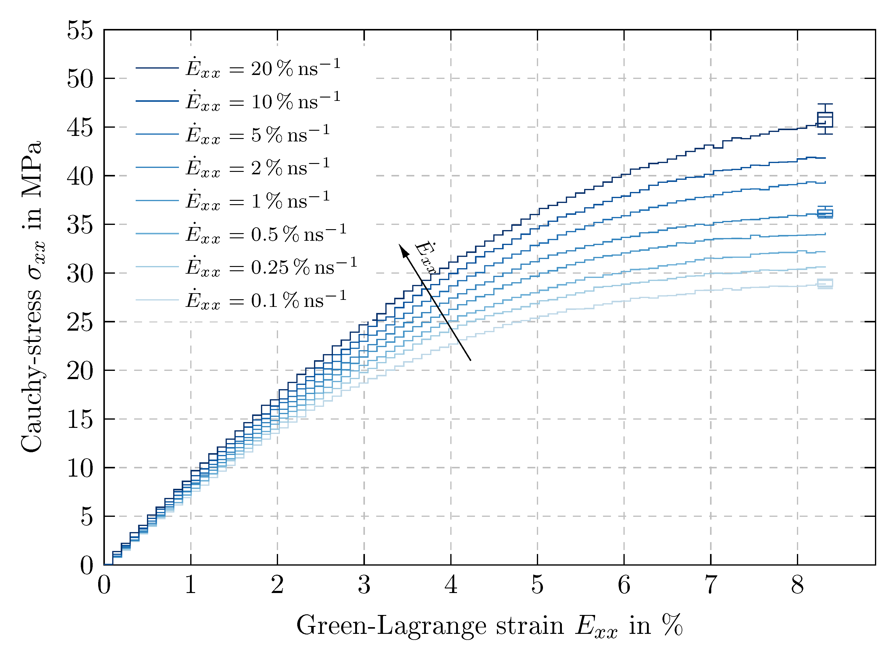
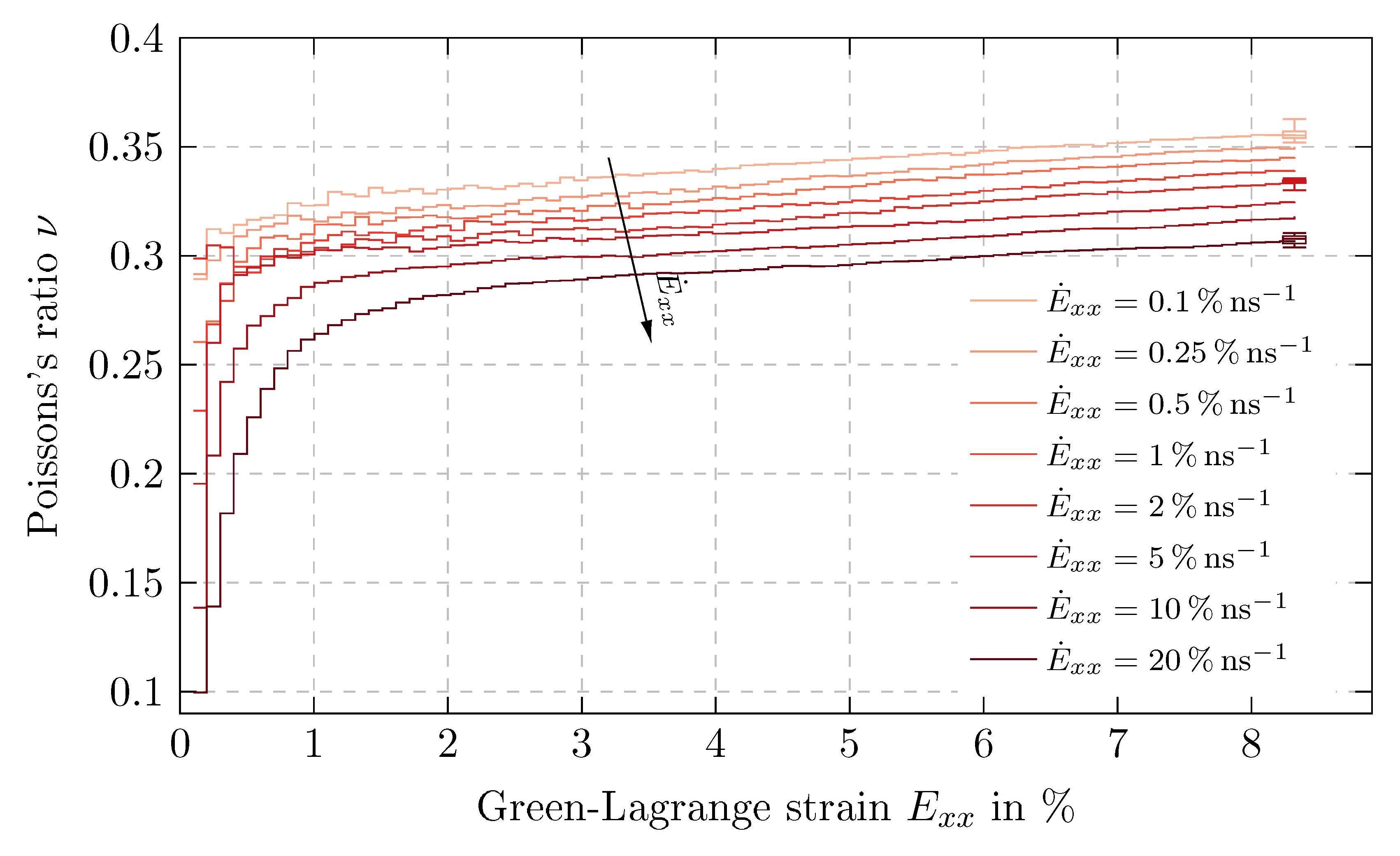
5.2. Results of Time Proportional Tests
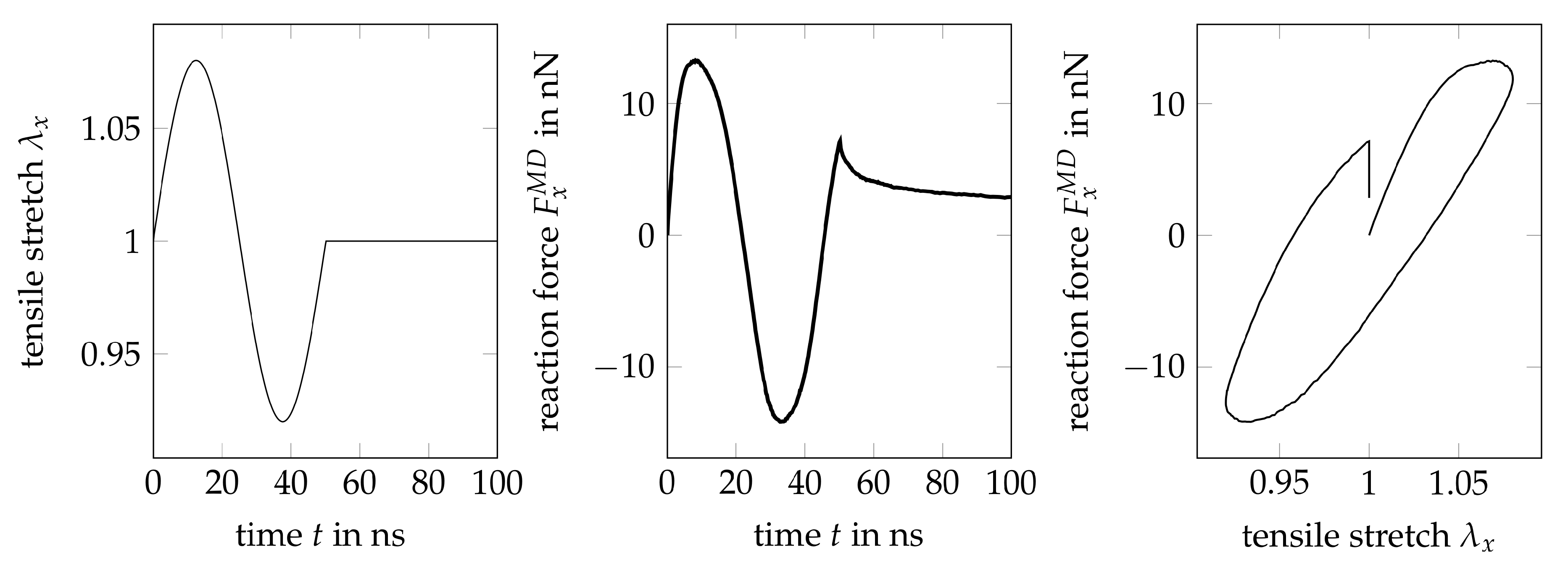
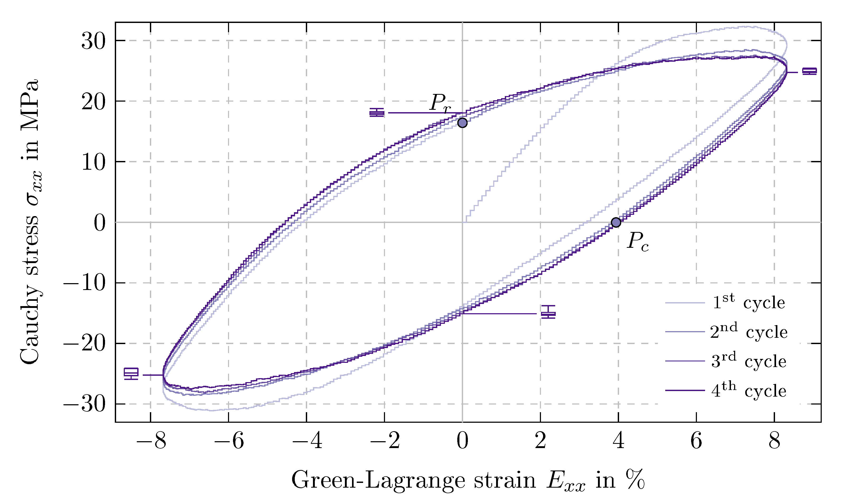
5.3. Results of Time Periodic Tests
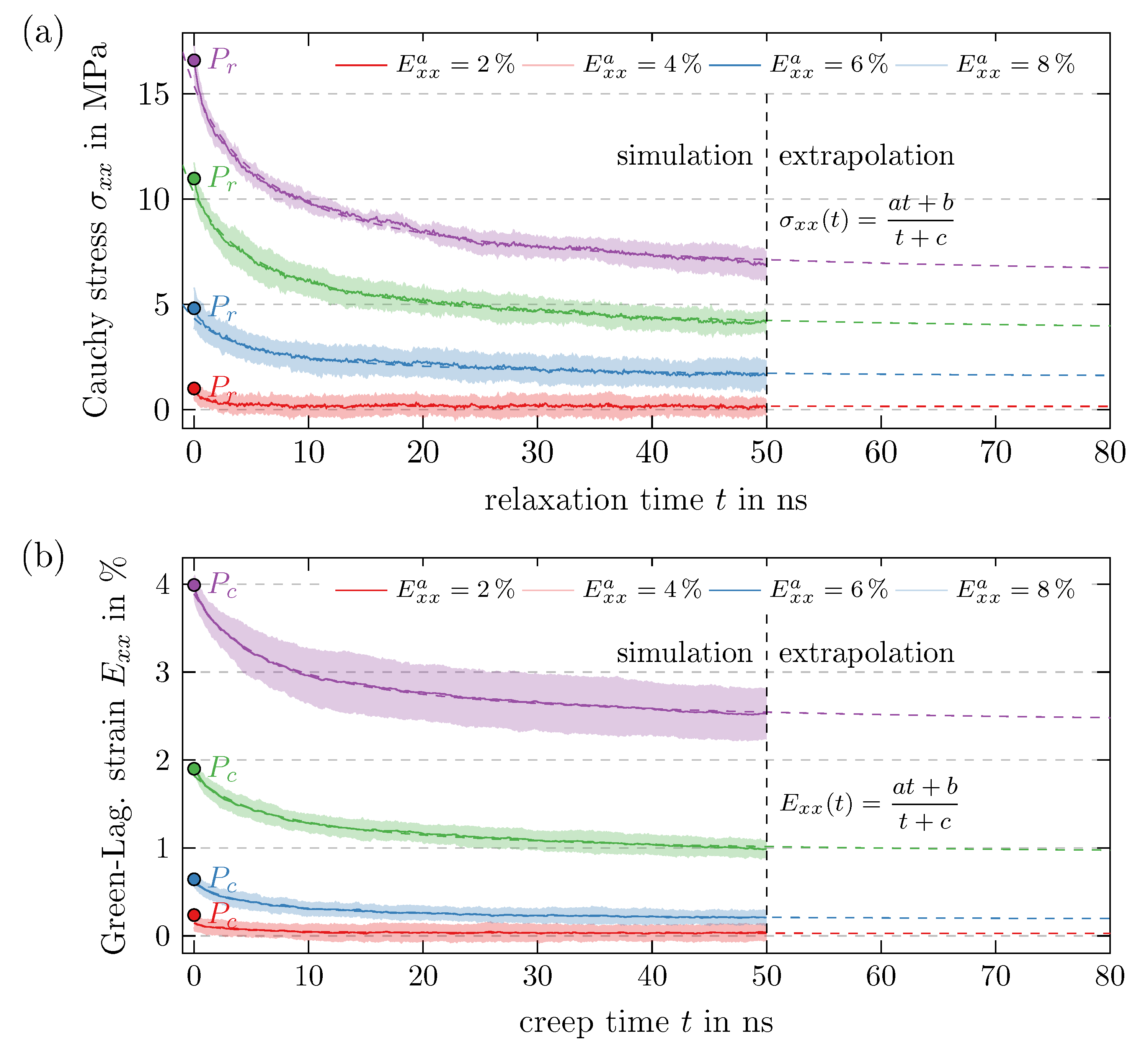
5.4. Stress Relaxation and Creep Tests
6. Exemplary Calibration of Continuum Mechanical Constitutive Laws by Means of MD-Data
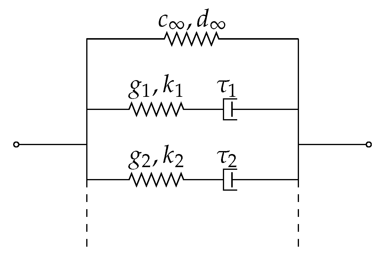
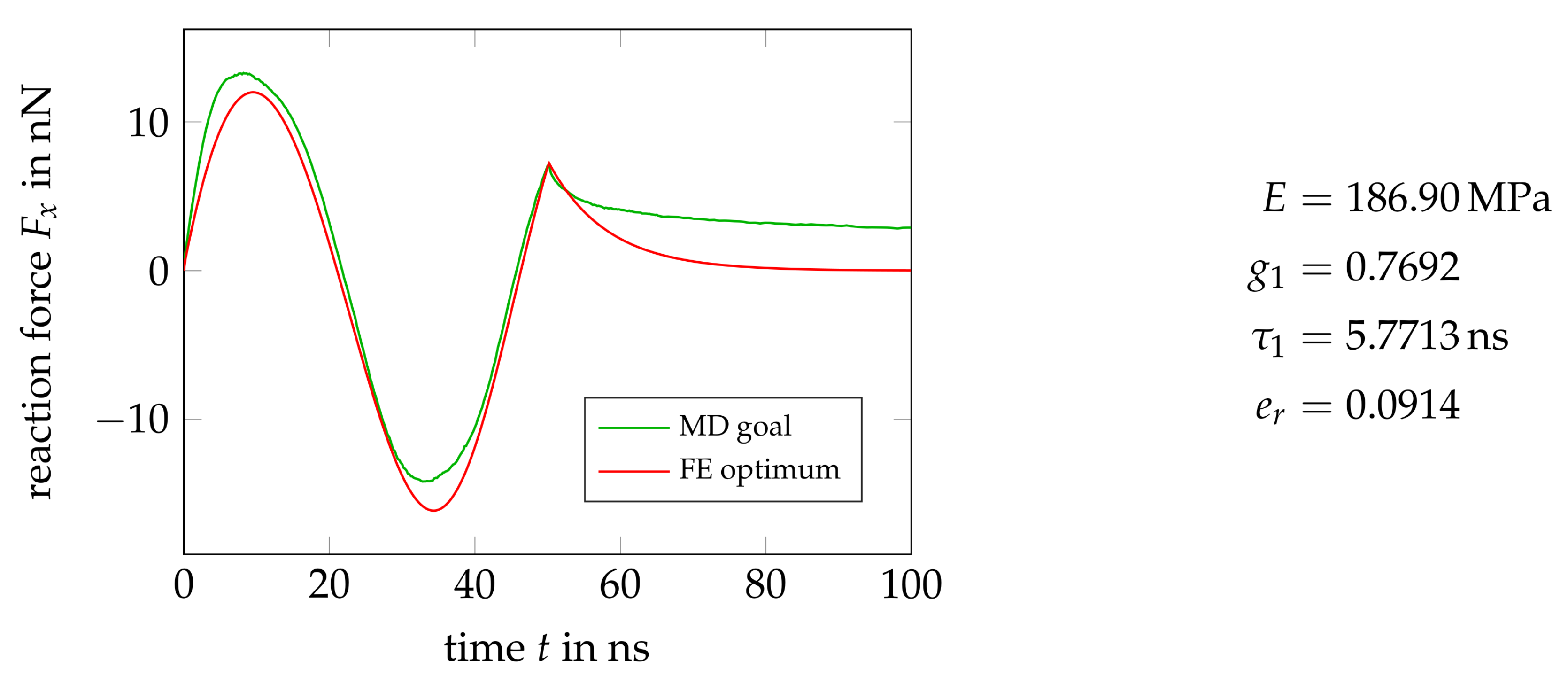
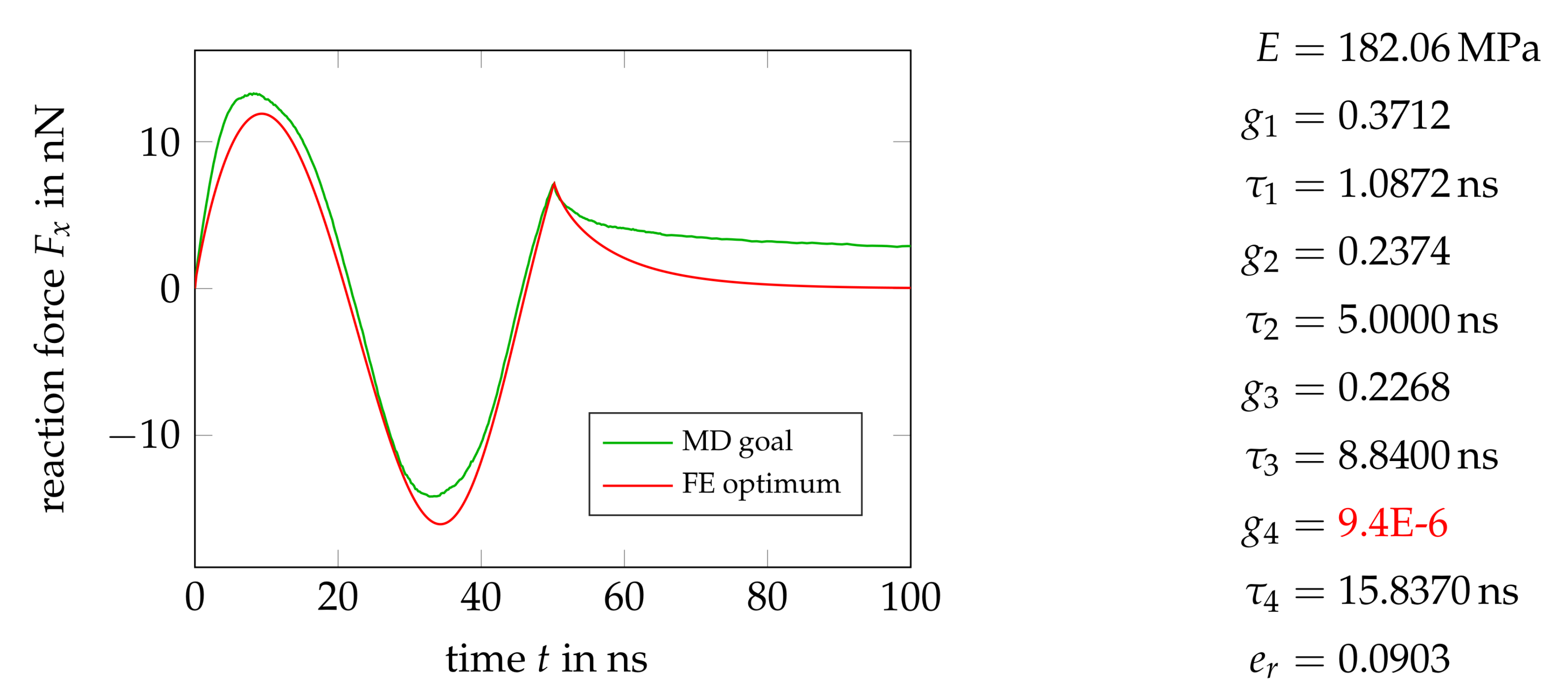
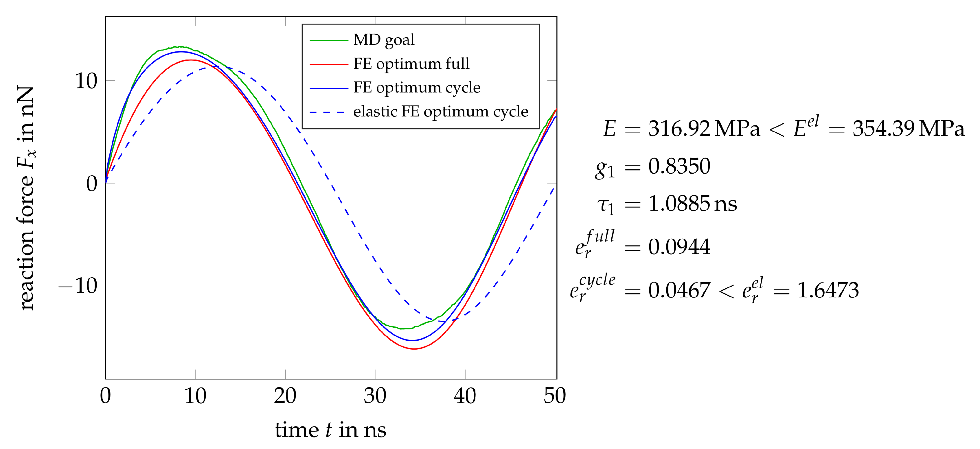
6.1. A Hyper-Viscoelastic Material Law: Neo-Hooke with Linear Maxwell Element(s)
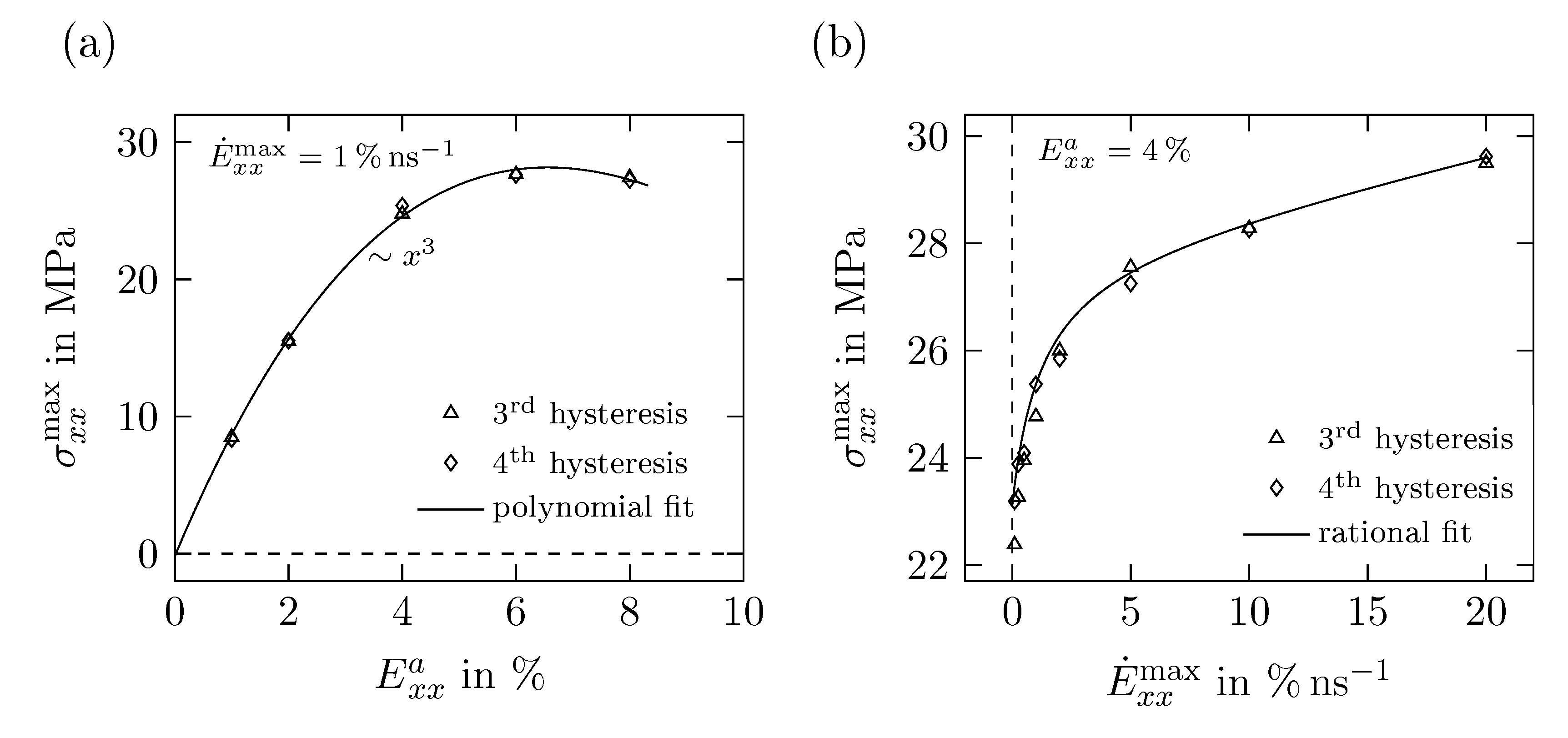
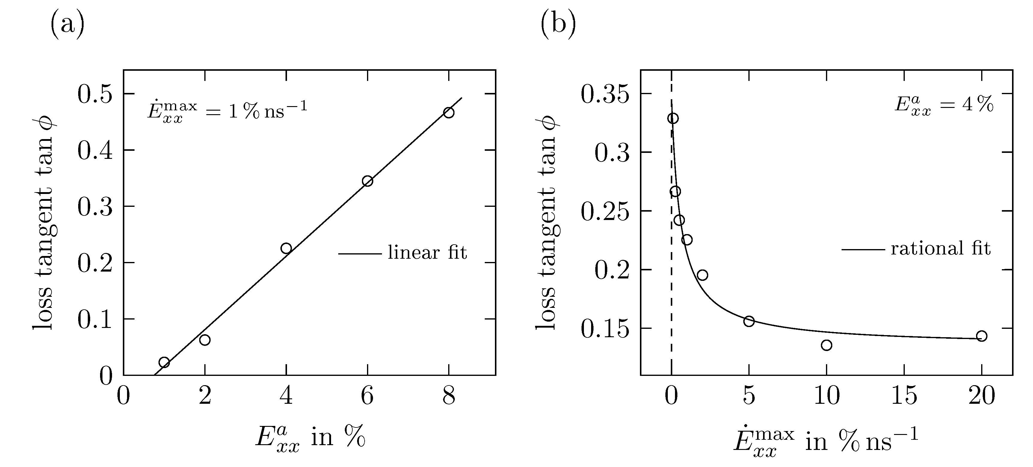
6.2. Results and Discussion
7. Conclusions and Outlook
Author Contributions
Funding
Acknowledgments
Conflicts of Interest
Abbreviations
| CG | Coarse-Grained |
| MD | Molecular Dynamics |
| PS | Polystyrene |
References
- Tadmor, E.B.; Miller, R.E. Modeling Materials—Continuum, Atomistic and Multiscale Techniques; Cambridge University Press: Cambridge, UK, 2011. [Google Scholar]
- Miller, R.E.; Tadmor, E. A unified framework and performance benchmark of fourteen multiscale atomistic/continuum coupling methods. Model. Simul. Mater. Sci. Eng. 2009, 17, 053001. [Google Scholar] [CrossRef]
- Vogiatzis, G.G.; Theodorou, D.N. Multiscale Molecular Simulations of Polymer-Matrix Nanocomposites. Arch. Comput. Methods Eng. 2018, 25, 591–645. [Google Scholar] [CrossRef] [PubMed]
- Semkiv, M.; Long, D.; Hütter, M. Concurrent two-scale model for the viscoelastic behavior of elastomers filled with hard nanoparticles. Contin. Mech. Thermodyn. 2016, 28, 1711–1739. [Google Scholar] [CrossRef] [Green Version]
- Bauman, P.T.; Oden, J.T.; Prudhomme, S. Adaptive multiscale modeling of polymeric materials with Arlequin coupling and Goals algorithms. Comput. Methods Appl. Mech. Eng. 2009, 198, 799–818. [Google Scholar] [CrossRef]
- Ben Dhia, H. Problèmes méchaniques multi-échelles: La méthode Arlequin. Comptes Rendus de l’Académie des Science, Series II b 1998, 326, 899–904. [Google Scholar]
- Ben Dhia, H.; Rateau, G. The Arlequin method as a flexible engineering design tool. Int. J. Numer. Methods Eng. 2005, 62, 1442–1462. [Google Scholar] [CrossRef]
- Ben Dhia, H.; Elkhodja, N.; Roux, F.X. Multimodeling of multi-alterated structures in the Arlequin framework. Solution with a Domain-Decomposition solver. Eur. J. Comput. Mech. 2008, 17, 969–980. [Google Scholar] [CrossRef]
- Pfaller, S.; Rahimi, M.; Possart, G.; Steinmann, P.; Müller-Plathe, F.; Böhm, M. An Arlequin-based method to couple molecular dynamics and finite element simulations of amorphous polymers and nanocomposites. Comput. Methods Appl. Mech. Eng. 2013, 260, 109–129. [Google Scholar] [CrossRef]
- Pfaller, S.; Possart, G.; Steinmann, P.; Rahimi, M.; Müller-Plathe, F.; Böhm, M. Investigation of interphase Effects in Silica-Polystyrene Nanocomposites Based on a Hybrid Molecular-Dynamics–Finite-Element Simulation Framework. Phys. Rev. E 2016, 93, 052505. [Google Scholar] [CrossRef]
- Liu, S.; Pfaller, S.; Rahimi, M.; Possart, G.; Steinmann, P.; Böhm, M.C.; Müller-Plathe, F. Uniaxial deformation of polystyrene–silica nanocomposites studied by hybrid molecular dynamics–finite element simulations. Comput. Mater. Sci. 2017, 129, 1–12. [Google Scholar] [CrossRef]
- Haupt, P. Continuum Mechanics and Theory of Materials; Springer Science & Business Media: Berlin/Heidelberg, Germany, 2013. [Google Scholar]
- Li, Y.; Tang, S.; Abberton, B.C.; Kröger, M.; Burkhart, C.; Jiang, B.; Papakonstantopoulos, G.J.; Poldneff, M.; Liu, W.K. A predictive multiscale computational framework for viscoelastic properties of linear polymers. Polymer 2012, 53, 5935–5952. [Google Scholar] [CrossRef]
- Rahimi, M.; Iriarte-Carretero, I.; Ghanbari, A.; Böhm, M.C.; Müller-Plathe, F. Mechanical behavior and interphase structure in a silica–polystyrene nanocomposite under uniaxial deformation. Nanotechnology 2012, 23, 305702. [Google Scholar] [CrossRef] [PubMed]
- Qian, H.J.; Carbone, P.; Chen, X.; Karimi-Varzaneh, H.A.; Liew, C.C.; Müller-Plathe, F. Temperature-transferable coarse-grained potentials for ethylbenzene, polystyrene, and their mixtures. Macromolecules 2008, 41, 9919–9929. [Google Scholar] [CrossRef]
- Ghanbari, A.; Ndoro, T.V.; Leroy, F.; Rahimi, M.; Böhm, M.C.; Müller-Plathe, F. Interphase structure in silica–polystyrene nanocomposites: A coarse-grained molecular dynamics study. Macromolecules 2011, 45, 572–584. [Google Scholar] [CrossRef]
- Reith, D.; Pütz, M.; Müller-Plathe, F. Deriving effective mesoscale potentials from atomistic simulations. J. Comput. Chem. 2003, 24, 1624–1636. [Google Scholar] [CrossRef] [PubMed] [Green Version]
- Milano, G.; Müller-Plathe, F. Mapping atomistic simulations to mesoscopic models: A systematic coarse-graining procedure for vinyl polymer chains. J. Phys. Chem. B 2005, 109, 18609–18619. [Google Scholar] [CrossRef] [PubMed]
- Müller-Plathe, F. Coarse-graining in polymer simulation: From the atomistic to the mesoscopic scale and back. ChemPhysChem 2002, 3, 754–769. [Google Scholar] [CrossRef]
- Karimi-Varzaneh, H.A.; van der Vegt, N.F.; Müller-Plathe, F.; Carbone, P. How good are coarse-grained polymer models? A comparison for atactic polystyrene. ChemPhysChem 2012, 13, 3428–3439. [Google Scholar] [CrossRef] [PubMed]
- Riccardi, E.; Böhm, M.C.; Müller-Plathe, F. Molecular dynamics method to locally resolve Poisson’s ratio: Mechanical description of the solid–soft-matter interphase. Phys. Rev. E 2012, 86, 036704. [Google Scholar] [CrossRef]
- Munaò, G.; Pizzirusso, A.; Kalogirou, A.; De Nicola, A.; Kawakatsu, T.; Müller-Plathe, F.; Milano, G. Molecular structure and multi-body potential of mean force in silica-polystyrene nanocomposites. Nanoscale 2018, 10, 21656–21670. [Google Scholar] [CrossRef] [Green Version]
- Farah, K.; Karimi-Varzaneh, H.A.; Müller-Plathe, F.; Böhm, M.C. Reactive molecular dynamics with material-specific coarse-grained potentials: growth of polystyrene chains from styrene monomers. J. Phys. Chem. B 2010, 114, 13656–13666. [Google Scholar] [CrossRef] [PubMed]
- Karimi-Varzaneh, H.A.; Qian, H.J.; Chen, X.; Carbone, P.; Müller-Plathe, F. IBIsCO: A molecular dynamics simulation package for coarse-grained simulation. J. Comput. Chem. 2011, 32, 1475–1487. [Google Scholar] [CrossRef] [PubMed]
- Lyulin, A.V.; Balabaev, N.K.; Michels, M. Molecular-weight and cooling-rate dependence of simulated Tg for amorphous polystyrene. Macromolecules 2003, 36, 8574–8575. [Google Scholar] [CrossRef]
- Lyulin, A.V.; Balabaev, N.K.; Mazo, M.A.; Michels, M. Molecular dynamics simulation of uniaxial deformation of glassy amorphous atactic polystyrene. Macromolecules 2004, 37, 8785–8793. [Google Scholar] [CrossRef]
- Kaliappan, S.K.; Cappella, B. Temperature dependent elastic–plastic behaviour of polystyrene studied using AFM force–distance curves. Polymer 2005, 46, 11416–11423. [Google Scholar] [CrossRef]
- Pfaller, S. Multiscale Simulation of Polymers—Coupling of Continuum Mechanics and Particle-Based Simulation. In Schriftenreihe Technische Mechanik; FAU Erlangen: Erlangen, Germany, 2015; Volume 16. [Google Scholar]
- Holzapfel, A.G. Nonlinear Solid Mechanics—A Continuum Approach for Engineering; John Wiley & Sons, Inc.: Hoboken, NJ, USA, 2000. [Google Scholar]
- Treloar, L.R.G. The Physics of Rubber Elasticity, 3rd ed.; Clarendon Press: Wotton-under-Edge, UK, 1975. [Google Scholar]
- Haupt, P. On the mathematical modelling of material behavior in continuum mechanics. Acta Mech. 1993, 100, 129–154. [Google Scholar] [CrossRef]
- Elias, H.G. An Introduction to Plastics; Wiley-VCH: Weinheim, Germany, 2003. [Google Scholar]
- McGill, R.; Tukey, J.W.; Larsen, W.A. Variations of box plots. Am. Stat. 1978, 32, 12–16. [Google Scholar]
- Brydson, J.A. Plastics Materials, 7th ed.; Butterworth-Heinemann: Oxford, UK, 1999. [Google Scholar]
- Brydson, J.A. Polymer Data Handbook; Brandrup, J., Immergut, E.H., Grulke, E.A., Abe, A., Bloch, D.R., Eds.; Oxford University Press: New York, NY, USA, 1999. [Google Scholar]
- Lemaitre, J.; Chaboche, J.L. Mechanics of Solid Materials; Cambridge University Press: Cambridge, UK, 1990. [Google Scholar]
- Bonet, J.; Wood, R.D. Nonlinear Continuum Mechanics for Finite Element Analysis; Cambridge University Press: Cambridge, UK, 2008. [Google Scholar]
- Tadmor, E.B.; Miller, R.E.; Elliott, R.S. Continuum Mechanics and Thermodynamics: From Fundamental Concepts to Governing Equations; Cambridge University Press: Cambridge, UK, 2012. [Google Scholar]
- Shaw, M.T.; MacKnight, W.J. Introduction to Polymer Viscoelasticity; John Wiley & Sons: Hoboken, NJ, USA, 2005. [Google Scholar]
- Savitzky, A.; Golay, M.J. Smoothing and differentiation of data by simplified least squares procedures. Anal. Chem. 1964, 36, 1627–1639. [Google Scholar] [CrossRef]
- Steinmann, P.; Hossain, M.; Possart, G. Hyperelastic models for rubber-like materials: consistent tangent operators and suitability for Treloar’s data. Arch. Appl. Mech. 2012, 82, 1183–1217. [Google Scholar] [CrossRef]
- Pfaller, S.; Kergaßner, A.; Steinmann, P. Optimisation of the Capriccio Method to Couple Particle-and-Continuum- Based Simulations of Polymers. Multiscale Sci. Eng. 2018, in press. [Google Scholar]


| 5 ps | |
| ps | |
| 5 ps | |
| 1 |
| (a) Time Proportional Load | |
| 1.08 | |
| 0.001 … | |
| 20000 , 40000 , 80000 | |
| … 50 fs | |
| (b) Time Periodic Load | |
| 0.01 … 0.08 | |
| 0.001 … | |
| 20000 | |
| … 50 fs | |
| (a) Relaxation | |||
| a | b | c | |
| % | – | ns | ns |
| 2 | 0.142 | 0.60 | 0.607 |
| 4 | 1.435 | 23.75 | 5.474 |
| 6 | 3.494 | 62.91 | 6.114 |
| 8 | 5.998 | 104.9 | 6.819 |
| (b) Creep | |||
| a | b | c | |
| % | MPa ns | MPa ns | ns |
| 2 | 0.0247 | 0.350 | 2.4 |
| 4 | 0.1721 | 2.943 | 4.908 |
| 6 | 0.8959 | 1.359 | 7.459 |
| 8 | 2.3630 | 2.621 | 6.738 |
© 2019 by the authors. Licensee MDPI, Basel, Switzerland. This article is an open access article distributed under the terms and conditions of the Creative Commons Attribution (CC BY) license (http://creativecommons.org/licenses/by/4.0/).
Share and Cite
Ries, M.; Possart, G.; Steinmann, P.; Pfaller, S. Extensive CGMD Simulations of Atactic PS Providing Pseudo Experimental Data to Calibrate Nonlinear Inelastic Continuum Mechanical Constitutive Laws. Polymers 2019, 11, 1824. https://doi.org/10.3390/polym11111824
Ries M, Possart G, Steinmann P, Pfaller S. Extensive CGMD Simulations of Atactic PS Providing Pseudo Experimental Data to Calibrate Nonlinear Inelastic Continuum Mechanical Constitutive Laws. Polymers. 2019; 11(11):1824. https://doi.org/10.3390/polym11111824
Chicago/Turabian StyleRies, Maximilian, Gunnar Possart, Paul Steinmann, and Sebastian Pfaller. 2019. "Extensive CGMD Simulations of Atactic PS Providing Pseudo Experimental Data to Calibrate Nonlinear Inelastic Continuum Mechanical Constitutive Laws" Polymers 11, no. 11: 1824. https://doi.org/10.3390/polym11111824
APA StyleRies, M., Possart, G., Steinmann, P., & Pfaller, S. (2019). Extensive CGMD Simulations of Atactic PS Providing Pseudo Experimental Data to Calibrate Nonlinear Inelastic Continuum Mechanical Constitutive Laws. Polymers, 11(11), 1824. https://doi.org/10.3390/polym11111824