Thermodynamics and Magnetic Excitations in Quantum Spin Trimers: Applications for the Understanding of Molecular Magnets

Abstract

Molecular magnets provide a playground of interesting phenomena and interactions that have direct applications for quantum computation and magnetic systems. A general understanding of the underlying geometries for molecular magnets therefore generates a consistent foundation for which further analysis and understanding can be established. Using a Heisenberg spin-spin exchange Hamiltonian, we investigate the evolution of magnetic excitations and thermodynamics of quantum spin isosceles trimers (two sides J and one side $\alpha J$) with increasing spin. For the thermodynamics, we produce exact general solutions for the energy eigenstates and spin decomposition, which can be used to determine the heat capacity and magnetic susceptibility quickly. We show how the thermodynamic properties change with $\alpha$ coupling parameters and how the underlying ground state governs the Schottky anomaly. Furthermore, we investigate the microscopic excitations by examining the inelastic neutron scattering excitations and structure factors. Here, we illustrate how the individual dimer subgeometry governs the ability for probing underlying excitations. Overall, we feel these calculations can help with the general analysis and characterization of molecular magnet systems.

1. Introduction

For over half a century, technology has been governed by the manipulation of the electron and its properties of charge and spin. Whether discussing the first transistor or the promise of quantum computation, the future of technology relies on the ability to take advantage of smaller quantum mechanical interactions for faster computer components, higher density memory, and larger data storage [1,2,3,4]. One method for data storage and quantum computation, is the property of spin, where the quest for smaller magnetic systems has lead to significant advances in the area of molecular magnets, which provide small nanomagnetic systems that can be used for quantum computation, spintronics, and magnetic storage [5,6,7]. However, the study of quantum spin clusters has been expanding and growing due to the possibilities of technological applications, quantum tunneling phenomenon, and interesting anisotropic effects.

Molecular magnets can be described as isolated magnetic clusters that are either part of a two- or three-dimensional lattice or be surrounded by non-magnetic ligands [8,9]. The latter are called single molecule magnets. In either case, molecular magnets produce low-energy, dispersionless excitations that provide avenues for many basic magnetic systems and devices [1]. Molecular magnetic systems are interesting due to their competition between ferromagnetic or antiferromagnetic interactions, which can lead to numerous varying ground states and quantum phase transitions [10,11].

While synthesis and characterization of molecular magnets are not trivial, throughout the last two decades, there have been hundreds of different molecular magnets studied through various techniques [12,13]. A variety of phenomena are probed through these techniques ranging from bulk properties (i.e., heat capacity, magnetic susceptibility, and the like) through magnetometry and electron spin resonance through microscopic properties (anisotropy and spin dynamics) using inelastic neutron scattering (INS) and optical spectroscopy [14,15,16,17,18,19,20,21]. On the theoretical end, there have been a number of experimental and theoretical studies on spin clusters and molecular magnets studying interactions and coupling aspects of these systems [22,23,24,25,26,27,28,29,30,31,32]. Furthermore, there have been advances in computational techniques to help identify and investigate interactions in molecular magnets through density functional theory [33]. Recently, computational databases have started to develop intricate tools to help identify new and distinct molecular magnets [34].

Recently, it has been shown that the larger molecule-based magnets have excitations that are characterized by the smaller subgeometries of the system [35,36,37]. This observation is important because it provides an opportunity to determine closed-form analytic solutions for systems that are typically solved numerically since most molecular magnetic systems are large clusters composed of high-spin atoms [30,32]. One can gain insight into larger clusters by thoroughly understanding the evolving excitations and transitions in smaller clusters [38].

In this study, we examine the effects of a variable dimer exchange embedded in a quantum spin trimer and verify that, regardless of spin and trimer geometry, the inelastic neutron scattering excitations for any trimer can be determined by the excitations of the individual bases. Furthermore, we examine the evolution of the thermodynamics as a function of spin and dimer exchange and show the quantum phase transition points in the heat capacity. These phase transitions allow for the possible tunability of quantum trimers with external fields (magnetic, strain, etc.)

2. The Heisenberg Trimer Model

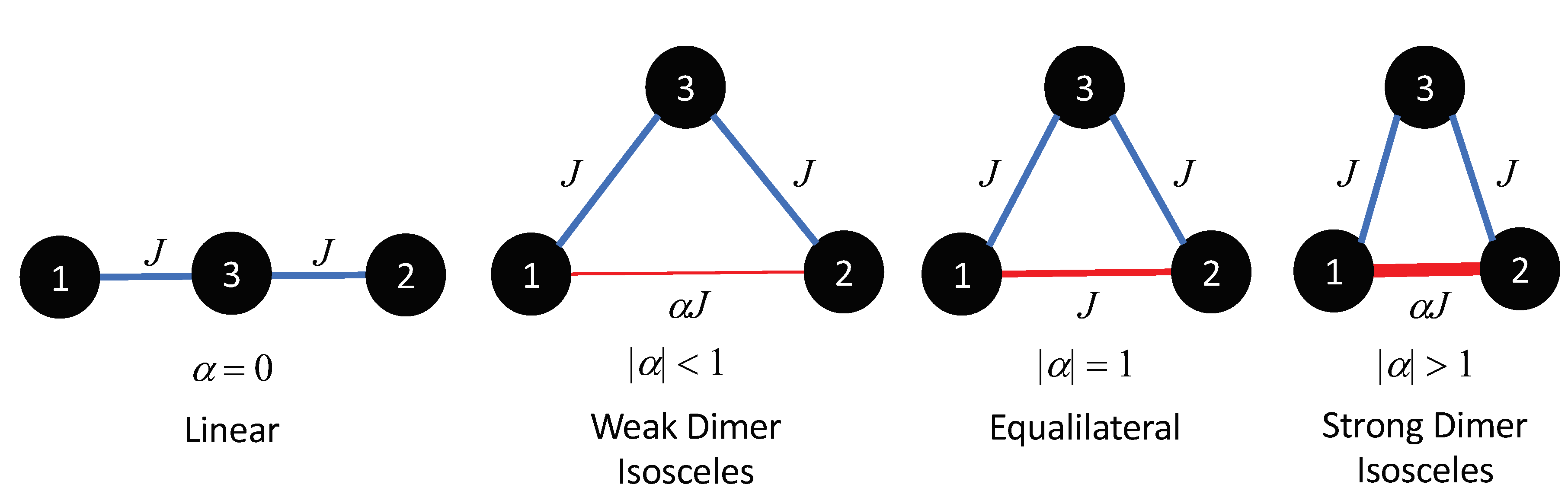
A trimer system consists of three interacting spins, where two of the interacting spins create a magnetic dimer. Figure 1 shows various magnetic isosceles trimer geometries with different dimer exchanges. Here, two sides of the trimer have an interaction of J, while the third side is a variational dimer exchange of $\alpha J$. When $\alpha$ = 0, the trimer is linear. However, as $|\alpha |$ is increased the system will produce a weak dimer, equilateral ($\alpha$ = 1), and a strong dimer ($|\alpha |>$ 1). It should be noted that the structural geometry is not dependent on the magnetic geometry.

Investigating the spin model for this geometry can include many different interactions and variations. However, in this study, the isotropic Heisenberg model is examined for various exchange interactions. Therefore, the Hamiltonian for the isosceles trimer we studied is

$$\mathcal{H}=\alpha J{\overrightarrow{\mathrm{S}}}_1·{\overrightarrow{\mathrm{S}}}_2+J({\overrightarrow{\mathrm{S}}}_2·{\overrightarrow{\mathrm{S}}}_3+{\overrightarrow{\mathrm{S}}}_3·{\overrightarrow{\mathrm{S}}}_1)$$

(1)

where J is the superexchange constant, $\alpha$ is the dimer exchange parameter, and S${}_i$ is the spin. For interactions in antiferromagnets $J>$0, while ferromagnets have $J<$ 0.

With the Hamiltonian, one can use exact diagonalization to find the energy eigenstates as well as the eigenfunctions for the Hamiltonian matrix. The energy states are critical for the thermodynamic properties, while the eigenfunctions or wavefunctions are needed to determine the inelastic neutron scattering cross sections. Due to the symmetry in this system, the energy of each magnetic state for the isosceles trimer can be written exactly using a spin total and spin dimer basis, where

$$E(S_t,S_d)=\frac{J}{2}\left[S_t(S_t+1)+S_d(S_d+1)(\alpha -1)-\alpha \left(S_1(S_1+1)+S_2(S_2+1)\right)-S_3(S_3+1)\right],$$

(2)

Here, S${}_t$ is the total spin of the trimer and S${}_d$ is the total spin for the dimer state. S${}_i$ is the spin for each of the magnetic atoms making the trimer. Therefore, from this, the energy for each state can be determined by knowing the total spin of trimer and dimer states for a given trimer of spin S.

To understand the spin components for each system, one must examine the spin decomposition of the trimer spin tensor product ($S\otimes S\otimes S$). From the trimer tensor product, one can decompose to an individual spin interacting with a spin dimer ($S\otimes (2S\oplus 2S-1\oplus 2S-2\oplus \dots \oplus 0)$). Therefore, the general trimer spin decomposition can be written as

$$3S\oplus {(3S-1)}^2\oplus {(3S-1)}^3\oplus \dots \oplus {(3S-2S)}^{2S+1}\oplus {(S-1)}^{2S-1}\oplus {(S-2)}^{2S-3}\oplus \dots \oplus {(S-N)}^{2(S-N)-1},$$

(3)

where N is S − 3/2 for half-integer spins and S − 1 for integer spin. The superscript denotes the multiplicity of the state. This summation can be simplified as

$$\sum _0^{2S}{(3S-N)}^{N+1}\oplus \sum _0^{\left[\right[S-1\left]\right]}{(S-N-1)}^{2(S-N)-1},$$

(4)

where the summations are sums over all direct sums and the second summation is for spins greater than 1/2. From this general direct sum, the total number of states can correctly be deduced from

$$\sum _0^{2S}(2(3S-N)+1)(N+1)+\sum _0^{\left[\right[S-1\left]\right]}(2(S-N-1)+1)(2(S-N)-1).$$

(5)

Once the sums are evaluated, the total number of states reduces to ${(2S+1)}^3$. From this spin decomposition, we can determine the spin state for any spin system. In this paper, we only examine up to spin 5/2, where the spin decomposition for each can be found in

Table 1. Spin decomposition and energy levels for the quantum spin trimers.

System	Dimer/Trimer States	Energy States (${\mathit{E}}_{{\mathit{S}}_{\mathit{t}},{\mathit{S}}_{\mathit{d}}}/\mathit{J}$)
$\frac{1}{2}\otimes \frac{1}{2}\otimes \frac{1}{2}$	$\begin{array}{c}1\oplus 0\\ \frac{3}{2}\oplus {\frac{1}{2}}^2\end{array}$	$\begin{array}{c}{E}_{3/2,1}/J=\frac{1}{4}(2+\alpha )\hfill \\ E_{1/2,1}/J=\frac{1}{4}(\alpha -4)\hfill \\ E_{1/2,0}/J=-\frac{3}{4}\alpha \hfill \end{array}$
$1\otimes 1\otimes 1$	$\begin{array}{c}2\oplus 1\oplus 0\\ 3\oplus 2^2\oplus 1^3\oplus 0\end{array}$	$\begin{array}{c}{E}_{3,2}/J=2+\alpha \hfill \\ E_{2,2}/J=\alpha -1\hfill \\ E_{1,2}/J=\alpha -3\hfill \\ E_{2,1}/J=1-\alpha \hfill \\ E_{1,1}/J=-1-\alpha \hfill \\ E_{1,0}/J=-2\alpha \hfill \\ E_{0,1}/J=-2-\alpha \hfill \end{array}$
$\frac{3}{2}\otimes \frac{3}{2}\otimes \frac{3}{2}$	$\begin{array}{c}3\oplus 2\oplus 1\oplus 0\\ \frac{9}{2}\oplus {\frac{7}{2}}^2\oplus {\frac{5}{2}}^3\oplus {\frac{3}{2}}^4\oplus {\frac{1}{2}}^2\end{array}$	$\begin{array}{cc}{E}_{9/2,3}/J=\frac{9}{4}(2+\alpha )\hfill & E_{3/2,2}/J=-3-\frac{3}{4}\alpha \hfill \\ E_{7/2,3}/J=\frac{9}{4}\alpha \hfill & E_{1/2,2}/J=-\frac{9}{2}-\frac{3}{4}\alpha \hfill \\ E_{5/2,3}/J=\frac{9}{4}(\alpha -\frac{14}{9})\hfill & E_{5/2,1}/J=\frac{3}{2}-\frac{11}{4}\alpha \hfill \\ E_{3/2,3}/J=\frac{9}{4}\alpha -6\hfill & E_{3/2,1}/J=-1-\frac{11}{4}\alpha \hfill \\ E_{7/2,2}/J=3-\frac{3}{4}\alpha \hfill & E_{1/2,1}/J=-\frac{5}{2}-\frac{11}{4}\alpha \hfill \\ E_{5/2,2}/J=-\frac{1}{2}-\frac{3}{4}\alpha \hfill & E_{3/2,0}/J=-\frac{15}{4}\alpha \hfill \end{array}$
$2\otimes 2\otimes 2$	$\begin{array}{c}4\oplus 3\oplus 2\oplus 1\oplus 0\\ 6\oplus 5^2\oplus 4^3\oplus 3^4\oplus 2^5\oplus 1^3\oplus 0\end{array}$	$\begin{array}{cc}{E}_{6,4}/J=4(2+\alpha )\hfill & E_{4,2}/J=4-3\alpha \hfill \\ E_{5,4}/J=2(1+2\alpha )\hfill & E_{3,2}/J=-3\alpha \hfill \\ E_{4,4}/J=4\alpha -3\hfill & E_{2,2}/J=-3-3\alpha \hfill \\ E_{3,4}/J=4\alpha -7\hfill & E_{1,2}/J=-5-3\alpha \hfill \\ E_{2,4}/J=4\alpha -10\hfill & E_{0,2}/J=-6-3\alpha \hfill \\ E_{5,3}/J=6\hfill & E_{3,1}/J=2-5\alpha \hfill \\ E_{4,3}/J=1\hfill & E_{2,1}/J=-1-5\alpha \hfill \\ E_{3,3}/J=-3\hfill & E_{1,1}/J=-3-5\alpha \hfill \\ E_{2,3}/J=-6\hfill & E_{2,0}/J=-6\alpha \hfill \\ E_{1,3}/J=-8\hfill \end{array}$
$\frac{5}{2}\otimes \frac{5}{2}\otimes \frac{5}{2}$	$\begin{array}{c}5\oplus 4\oplus 3\oplus 2\oplus 1\oplus 0\\ \frac{15}{2}\oplus {\frac{13}{2}}^2\oplus {\frac{11}{2}}^3\oplus {\frac{9}{2}}^4\oplus {\frac{7}{2}}^5\oplus {\frac{5}{2}}^6\oplus {\frac{3}{2}}^4\oplus {\frac{1}{2}}^2\end{array}$	$\begin{array}{cc}{E}_{15/2,5}/J=\frac{25}{4}(2+\alpha )\hfill & E_{7/2,3}/J=-\frac{5}{2}-\frac{11}{4}\alpha \hfill \\ E_{13/2,5}/J=5+\frac{25}{4}\alpha \hfill & E_{5/2,3}/J=-6-\frac{11}{4}\alpha \hfill \\ E_{11/2,5}/J=-\frac{3}{2}+\frac{25}{4}\alpha \hfill & E_{3/2,3}/J=-\frac{17}{2}-\frac{11}{4}\alpha \hfill \\ E_{9/2,5}/J=\frac{25}{4}\alpha -7\hfill & E_{1/2,3}/J=-10-\frac{11}{4}\alpha \hfill \\ E_{7/2,5}/J=\frac{25}{4}\alpha -\frac{23}{4}\hfill & E_{9/2,2}/J=2-\frac{11}{4}\alpha \hfill \\ E_{5/2,5}/J=\frac{25}{4}\alpha -15\hfill & E_{7/2,2}/J=\frac{1}{2}-\frac{23}{4}\alpha \hfill \\ E_{13/2,4}/J=10+\frac{5}{4}\alpha \hfill & E_{5/2,2}/J=-3-\frac{23}{4}\hfill \\ E_{11/2,4}/J=\frac{7}{2}+\frac{5}{4}\alpha \hfill & E_{3/2,2}/J=-\frac{11}{2}-\frac{23}{4}\alpha \hfill \\ E_{9/2,4}/J=\frac{5}{4}\alpha -2\hfill & E_{1/2,2}/J=-7-\frac{23}{4}\alpha \hfill \\ E_{7/2,4}/J=\frac{5}{4}\alpha -\frac{13}{2}\hfill & E_{7/2,1}/J=\frac{5}{2}-\frac{31}{4}\alpha \hfill \\ E_{5/2,4}/J=\frac{5}{4}\alpha -10\hfill & E_{5/2,1}/J=-1-\frac{31}{4}\alpha \hfill \\ E_{3/2,4}/J=\frac{5}{4}\alpha -\frac{25}{2}\hfill & E_{3/2,1}/J=-\frac{7}{2}-\frac{31}{4}\alpha \hfill \\ E_{11/2,3}/J=\frac{15}{2}-\frac{11}{4}\alpha \hfill & E_{5/2,0}/J=-\frac{35}{4}\alpha \hfill \\ E_{9/2,3}/J=2-\frac{11}{4}\alpha \hfill \end{array}$

. However, the general S equations can be used for any spin.

In the S = 1/2 case, you have a S = 1/2 dimer which has spin states of (1 and 0). Adding a third spin to make the trimer produces three spin total states one S${}_t$ = 3/2 state and two S${}_t$ = 1/2 states, where the two S = 1/2 states have different dimer bases of S${}_d$ = 1 and 0. The energy states for the S = 1/2, 1, 3/2, 2, and 5/2 trimers are given in Table 1.

3. Evolution of the Thermodynamic Properties

The following sections show the calculations for the spin states of isosceles trimers of S = 1/2, S = 1, S = 3/2, S = 2, and S = 5/2. As the spin increases, the spin states drastically increase in size and complexity. These calculations are used in the sections following to find the energy levels, partition function, heat capacity, and later the magnetic susceptibility.

Using the energy eigenstates and eigenvalues in Table 1, we can determine the partition function of the system using

$$Z=\sum _{i=1}^N{e}^{-\beta {\mathrm{E}}_{\mathrm{i}}}=\sum _{{\mathrm{E}}_{\mathrm{i}}}(2{\mathrm{S}}_{tot}+1)e^{-\beta {\mathrm{E}}_{\mathrm{i}}},$$

(6)

where the sum $i=1\cdots N$ is over all N independent energy eigenstates (including magnetic substates), the sum ${\sum }_{{\mathrm{E}}_{\mathrm{i}}}$ is over energy levels only, and $\beta$ = 1/k${}_b$T. In practice, we will employ the usual set of $\widehat{z}$-polarized magnetic basis states.

While the general definition of the heat capacity can be simply described as the amount of energy required to raise the temperature of a material by a small amount (assuming adiabatic conditions) [39]. The more rigorous definition can be found by through the manipulation of the partition function shown as

$$C=k_B{\beta }^2\frac{d^{2}ln(Z)}{d{\beta }^2}.$$

(7)

Although the heat capacity is an important property, the overall size of the functions makes them difficult to report. Most mathematical packages, however, would be able to calculate this property once the partition function is determined from the energy states. The heat capacity has a distinct feature, known as the Schottky anomaly, which has a characteristic $\lambda$ shape, that denotes a change in entropy of the quantum system, which happens in the transition from an antiferromagnetic or ferromagnetic ground state to a thermally excited state at higher temperatures. This thermal activity eventually leads to a paramagnetic state due to the thermal fluctuations of the spins.

In most magnetic systems, the transition is a second-order continuous transition. Because of this, if one integrates the ratio of the heat capacity and $\beta$ over all temperatures, then the total entropy of the system can be calculated. From statistical mechanics, the total entropy will be equal to the ratio of the dimensionality of the Hilbert space (N) over the degeneracy of the ground state ($N_0$) [31,39], which is written as

$$S={\int }_0^{\infty }\frac{C}{\beta }d\beta =k_B\ln \left(\frac{N}{N_0}\right).$$

(8)

This allows one to verify the energy eigenstates through a determination of the entropy.

When a magnetic field is applied to a material, the magnetic moments in a lattice arrangement at a certain temperature T react by either lining up to point in the same direction (ferromagnetic) or lining up in opposite directions (antiferromagnetic). The response of the material to the magnetic field applied is its magnetic susceptibility [39]. The energy eigenvalues can be used to find the magnetic susceptibility, which is given by

$$\chi =\frac{\beta }{Z}\sum _{i=1}^N{(M_z^2)}_i{e}^{-\beta {\mathrm{E}}_{\mathrm{i}}}=\frac{1}{3}{(g{\mu }_B)}^2\frac{\beta }{Z}\sum _{{\mathrm{E}}_{\mathrm{i}}}(2{\mathrm{S}}_{tot}+1)({\mathrm{S}}_{tot}+1){\mathrm{S}}_{tot}{e}^{-\beta {\mathrm{E}}_{\mathrm{i}}},$$

(9)

In these formulas $M_z=mg{\mu }_B$ where $m={\mathrm{S}}_{\mathrm{tot}}^{\mathrm{z}}/\mathsf{\hslash }$ is the integral or half-integral magnetic quantum number, and g is the electron g-factor. The magnetic susceptibility allows one to clearly determine the total spin of the ground state; the larger the total spin the larger the magnetic susceptibility at T = 0.

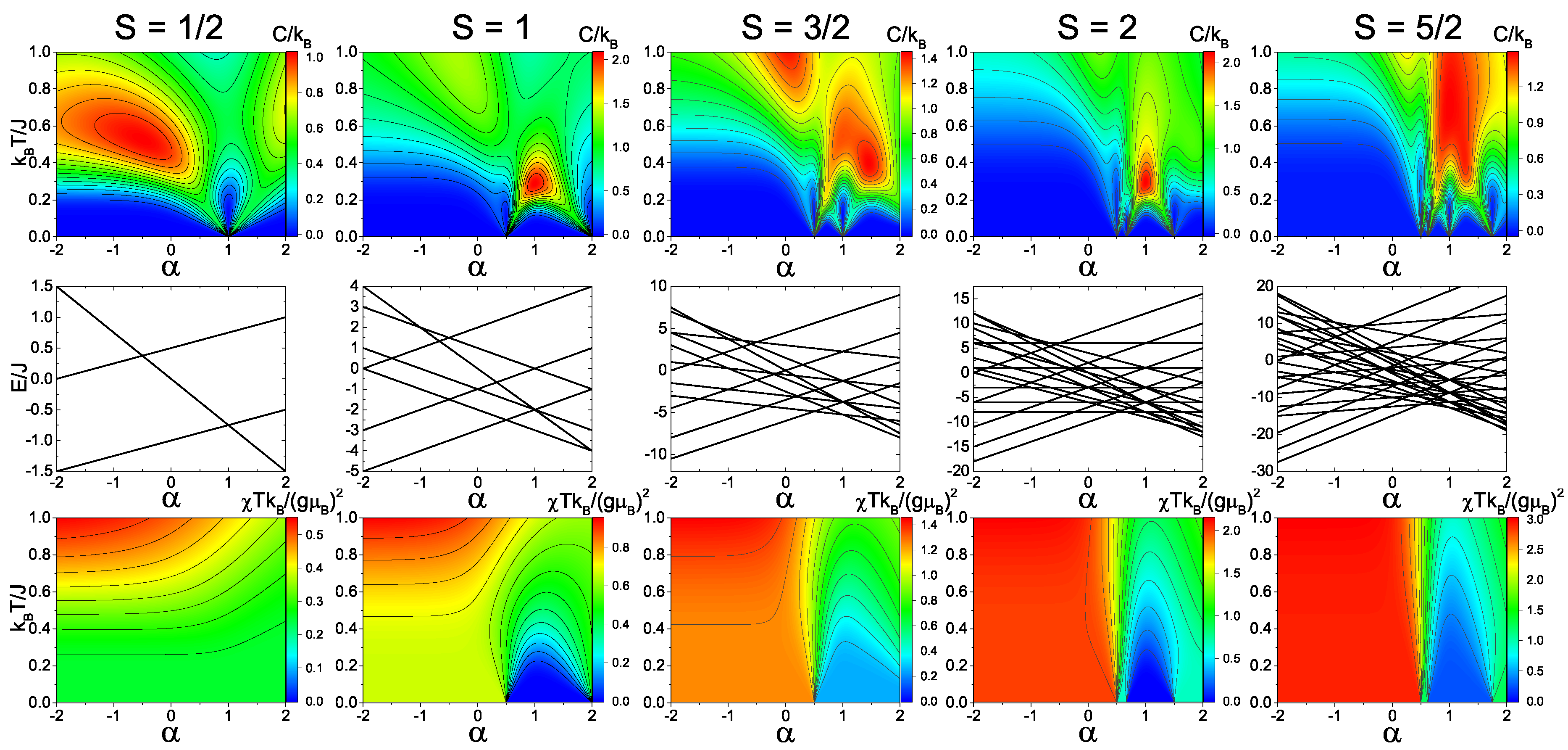
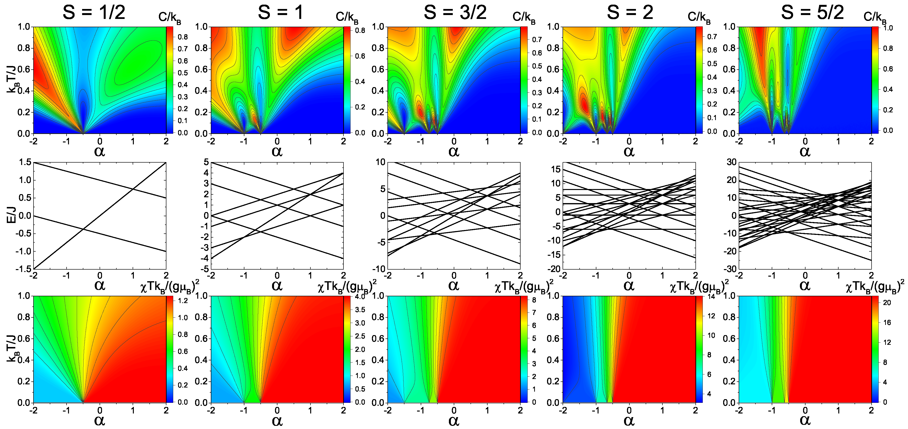
Figure 2 and Figure 3 show the calculated heat capacity, energy levels, and magnetic susceptibility as a function of temperature and dimer exchange ($\alpha$) for S = 1/2, 1, 3/2, 2, and 5/2 spin trimers with antiferromagnetic and ferromagnetic, respectively.

For the antiferromagnetic spin-1/2 model (Figure 2), there is a distinct quantum phase transition at $\alpha$ = 1. At this transition point, the system does not shift its spin total state of 1/2. However, the spin dimer state does shift from spin 1 to spin 0. The phase transition is clearly shown in the heat capacity due to the shift in the temperature dependence of the Schottky anomaly at the transition point. Since the quantum phase transition is not a shift in total spin, the magnetic susceptibility does not have any major shift. In the ferromagnetic spin-1/2 model (Figure 3), the quantum transition shifts to $\alpha$ = −0.5. Unlike the antiferromagnetic spin-1/2 model, however, the ferromagnetic case has a distinct shift in total spin from spin 1/2 to spin 3/2, which is evident in both the heat capacity and magnetic susceptibility.

In the antiferromagnetic spin-1 model (Figure 2), there are two quantum phase transition points which correspond to the shifts in the total spin S${}_t$ = 1 to 0 ($\alpha$ = 0.5) and from S${}_t$ = 0 to 1 ($\alpha$ = 2). This transition is shown in both the heat capacity and magnetic susceptibility, where the magnetic susceptibility of the spin-0 state goes to zero as the temperature approaches zero. In the ferromagnetic spin-1 model (Figure 3), there are also two phase transitions that have a ground states shift from S${}_t$ = 1 to 2 ($\alpha$ = −1.0) and from S${}_t$ = 2 to 3 ($\alpha$ = −0.5), which is evident from the magnetic susceptibility.

In the spin-3/2, spin-2, and spin-5/2 models, there are multiple quantum phase transitions in the energy spectra that correspond to distinct changes in the heat capacity and magnetic susceptibility. From Figure 2 and Figure 3, it is clear that the peak of the Schottky anomaly is directly related to the energy gap between the ground state and first excited state of the given magnetic system. Overall, these transitions allow for possible switch points in systems where $\alpha$ is variable with applied external fields. By switching the ground state with an external field, the change in the magnetization can lead to an increase or decrease in magnetic moment, which will designate the ground state and provide the state, therefore acting as a spin switch.

4. Inelastic Neutron Scattering Structure Factors

While the heat capacity and magnetic susceptibility can provide detailed information about the total spin states and quantum transition in the trimer system, inelastic neutron scattering (INS) allows for the examination of the magnetic states on a microscopic level, where it measures characteristic geometries and excitations for the trimer systems. In addition, therefore, to the calculated bulk properties, we also examined results for inelastic neutron scattering intensities.

As discussed in [31], in ”spin-only” magnetic neutron scattering at T = 0, the inelastic magnetic scattering of an incident neutron will have a differential cross section that is proportional to the unpolarized neutron scattering structure factor

$$S_{ba}(\overrightarrow{q},\omega )={\int }_{-\infty }^{\infty }\frac{dt}{2\pi }\sum _{\overrightarrow{x}{}_i,\overrightarrow{x}{}_j}{e}^{i\overrightarrow{q}·({\overrightarrow{x}}_i-{\overrightarrow{x}}_j)+i\omega t}〈{\mathsf{\Psi }}_j|{\mathrm{S}}_b^{†}({\overrightarrow{x}}_j,t){\mathrm{S}}_a({\overrightarrow{x}}_i,0)|{\mathsf{\Psi }}_i〉.$$

(10)

where the system has an initial state $|{\mathsf{\Psi }}_i\rangle$, with momentum transfer $\mathsf{\hslash }\overrightarrow{q}$ and energy transfer $\mathsf{\hslash }\omega$. Here, the site sums in Equation (10) run over all magnetic ions in one unit cell, where $a,b$ are the spatial indices of the spin operators and ${\overrightarrow{x}}_i$ are the spatial vectors for the spin sites.

Since spin clusters have transitions between discrete energy levels, the time integral in the energy transfer gives a trivial delta function $\delta$(E${}_f$− E${}_i$−$\mathsf{\hslash }\omega$). We can therefore shift to an “exclusive structure factor” for the individual excitation of states $\lambda$ within a specific magnetic multiplet, $|{\mathsf{\Psi }}_f({\lambda }_f)\rangle$, from the given initial state $|{\mathsf{\Psi }}_i\rangle$. This structure factor can be written as

$$S_{ba}^{(fi)}(\overrightarrow{q})=\sum _{{\lambda }_f}\langle {\mathsf{\Psi }}_i|V_b^{†}|{\mathsf{\Psi }}_f({\lambda }_f)\rangle \langle {\mathsf{\Psi }}_f({\lambda }_f)|V_a|{\mathsf{\Psi }}_i\rangle ,$$

(11)

where the vector $V_a(\overrightarrow{q})$ is a sum of spin operators over all magnetic ions in a unit cell,

$$V_a=\sum _{{\overrightarrow{x}}_i}{\mathrm{S}}_a({\overrightarrow{x}}_i)e^{i\overrightarrow{q}·{\overrightarrow{x}}_i}.$$

(12)

Assuming an isotropic magnetic Hamiltonian with a spherical basis for the spin operators S${}_a$, the tensor $S_{ba}^{(fi)}(\overrightarrow{q})$ is diagonal and has entries that are proportional to a universal function of $\overrightarrow{q}$ times a product of Clebsch–Gordon coefficients [21,31]. The structure factor can then be simplified by examining the unpolarized result $\langle S_{ba}^{(fi)}(\overrightarrow{q})\rangle$, which is obtained by averaging over all polarizations. Since the unpolarized $\langle S_{ba}^{(fi)}(\overrightarrow{q})\rangle$ is proportional to ${\delta }_{ab}$, the structure factor can be given by the function $S(\overrightarrow{q})$;

$$\langle S_{ba}^{(fi)}(\overrightarrow{q})\rangle ={\delta }_{ab}S(\overrightarrow{q})\propto \sum _{{\lambda }_i,{\lambda }_f}\langle {\mathsf{\Psi }}_i({\lambda }_i)|V_b^{†}|{\mathsf{\Psi }}_f({\lambda }_f)\rangle \langle {\mathsf{\Psi }}_f({\lambda }_f)|V_a|{\mathsf{\Psi }}_i({\lambda }_i)\rangle .$$

(13)

This function provides us with the overall functional form of the INS structure factors.

Since many molecular magnetic systems are not a single crystal sample, but typically powder, the result given above can be reduced to the powder average by integrating the structure factor over all angles [21,31], which is given by

$$\overline{S}(q)=\int \frac{d{\mathsf{\Omega }}_{\widehat{q}}}{4\pi }S(\overrightarrow{q}).$$

(14)

While we use this methodology to determine the complete INS structure factor, we are really more interested in the functional form of the structure factor as it provides information on excitations of the system according to spatial parameters and the excited subgeometries for the trimer system.

In

Table 2. Inelastic neutron scattering (INS) energy excitations and structure factors.

System	Transition $|{\mathsf{\Psi }}_{{\mathit{S}}_{\mathit{t}},{\mathit{S}}_{\mathit{d}}}\rangle \to |{\mathsf{\Psi }}_{{\mathit{S}}_{\mathit{t}},{\mathit{S}}_{\mathit{d}}}\rangle$	$\mathsf{\Delta }\mathit{E}$${}^1$	Structure Factors ${}^{2,3}$
Spin 1/2 Trimer	$|{\mathsf{\Psi }}_{1/2,0}\rangle \to |{\mathsf{\Psi }}_{1/2,1}\rangle$	$(\alpha -1)J$	$\frac{1}{6}$(1 − cos($\overrightarrow{q}·{\overrightarrow{r}}_{12}$))
	$|{\mathsf{\Psi }}_{1/2,0}\rangle \to |{\mathsf{\Psi }}_{3/2,1}\rangle$	$(\frac{1}{2}+\alpha )J$	$\frac{1}{3}$(1 − cos($\overrightarrow{q}·{\overrightarrow{r}}_{12}$))
	$|{\mathsf{\Psi }}_{1/2,1}\rangle \to |{\mathsf{\Psi }}_{3/2,1}\rangle$	$\frac{3}{2}J$	$\frac{1}{3}$(3 + cos($\overrightarrow{q}·{\overrightarrow{r}}_{12}$) − 2cos($\overrightarrow{q}·{\overrightarrow{r}}_{23}$) − 2cos($\overrightarrow{q}·{\overrightarrow{r}}_{31}$))
Spin 1 Isosceles Trimer	$|{\mathsf{\Psi }}_{0,1}\rangle \to |{\mathsf{\Psi }}_{1,2}\rangle$	$(2\alpha -1)J$	$\frac{5}{9}$(1 − cos($\overrightarrow{q}·{\overrightarrow{r}}_{12}$))
	$|{\mathsf{\Psi }}_{0,1}\rangle \to |{\mathsf{\Psi }}_{1,1}\rangle$	J	$\frac{1}{3}$(3 + cos($\overrightarrow{q}·{\overrightarrow{r}}_{12}$) − 2cos($\overrightarrow{q}·{\overrightarrow{r}}_{23}$) − 2cos($\overrightarrow{q}·{\overrightarrow{r}}_{31}$))
	$|{\mathsf{\Psi }}_{0,1}\rangle \to |{\mathsf{\Psi }}_{1,0}\rangle$	$(2-\alpha )J$	$\frac{4}{9}$(1 − cos($\overrightarrow{q}·{\overrightarrow{r}}_{12}$))
	$|{\mathsf{\Psi }}_{1,2}\rangle \to |{\mathsf{\Psi }}_{1,1}\rangle$	$(2-2\alpha )J$	$\frac{5}{36}$(1 − cos($\overrightarrow{q}·{\overrightarrow{r}}_{12}$))
	$|{\mathsf{\Psi }}_{1,2}\rangle \to |{\mathsf{\Psi }}_{1,0}\rangle$	$(3-3\alpha )J$	0
	$|{\mathsf{\Psi }}_{1,2}\rangle \to |{\mathsf{\Psi }}_{2,2}\rangle$	$2J$	$\frac{3}{40}$(3 + cos($\overrightarrow{q}·{\overrightarrow{r}}_{12}$) − 2cos($\overrightarrow{q}·{\overrightarrow{r}}_{23}$) − 2cos($\overrightarrow{q}·{\overrightarrow{r}}_{31}$))
	$|{\mathsf{\Psi }}_{1,2}\rangle \to |{\mathsf{\Psi }}_{2,1}\rangle$	$(4-2\alpha )J$	$\frac{1}{180}$(1 − cos($\overrightarrow{q}·{\overrightarrow{r}}_{12}$))
	$|{\mathsf{\Psi }}_{1,1}\rangle \to |{\mathsf{\Psi }}_{1,0}\rangle$	$(1-\alpha )J$	1 − cos($\overrightarrow{q}·{\overrightarrow{r}}_{12}$)
	$|{\mathsf{\Psi }}_{1,1}\rangle \to |{\mathsf{\Psi }}_{2,2}\rangle$	$2\alpha J$	1 − cos($\overrightarrow{q}·{\overrightarrow{r}}_{12}$)
	$|{\mathsf{\Psi }}_{1,1}\rangle \to |{\mathsf{\Psi }}_{2,1}\rangle$	$2J$	3 + cos($\overrightarrow{q}·{\overrightarrow{r}}_{12}$) − 2cos($\overrightarrow{q}·{\overrightarrow{r}}_{23}$) − 2cos($\overrightarrow{q}·{\overrightarrow{r}}_{31}$)
	$|{\mathsf{\Psi }}_{1,0}\rangle \to |{\mathsf{\Psi }}_{2,2}\rangle$	$(3\alpha -1)J$	0
	$|{\mathsf{\Psi }}_{1,0}\rangle \to |{\mathsf{\Psi }}_{2,1}\rangle$	$(1-3\alpha )J$	1 − cos($\overrightarrow{q}·{\overrightarrow{r}}_{12}$)
Spin 3/2 Isosceles Trimer	$|{\mathsf{\Psi }}_{1/2,2}\rangle \to |{\mathsf{\Psi }}_{1/2,1}\rangle$	$(2-2\alpha )J$	(1 − cos($\overrightarrow{q}·{\overrightarrow{r}}_{12}$))
	$|{\mathsf{\Psi }}_{1/2,2}\rangle \to |{\mathsf{\Psi }}_{3/2,3}\rangle$	$(3\alpha -\frac{3}{2})J$	$\frac{21}{40}$(1 − cos($\overrightarrow{q}·{\overrightarrow{r}}_{12}$))
	$|{\mathsf{\Psi }}_{1/2,2}\rangle \to |{\mathsf{\Psi }}_{3/2,2}\rangle$	$\frac{3}{2}J$	$\frac{3}{8}$(3 + cos($\overrightarrow{q}·{\overrightarrow{r}}_{12}$) − 2cos($\overrightarrow{q}·{\overrightarrow{r}}_{23}$) − 2cos($\overrightarrow{q}·{\overrightarrow{r}}_{31}$))
	$|{\mathsf{\Psi }}_{1/2,2}\rangle \to |{\mathsf{\Psi }}_{3/2,1}\rangle$	$(\frac{7}{2}-2\alpha )J$	$\frac{3}{40}$(1 − cos($\overrightarrow{q}·{\overrightarrow{r}}_{12}$))
	$|{\mathsf{\Psi }}_{1/2,2}\rangle \to |{\mathsf{\Psi }}_{3/2,0}\rangle$	$(\frac{9}{2}-3\alpha )J$	0
	$|{\mathsf{\Psi }}_{1/2,1}\rangle \to |{\mathsf{\Psi }}_{3/2,3}\rangle$	$(5\alpha -\frac{7}{2})J$	0
	$|{\mathsf{\Psi }}_{1/2,1}\rangle \to |{\mathsf{\Psi }}_{3/2,2}\rangle$	$(2\alpha -\frac{1}{2})J$	1 − cos($\overrightarrow{q}·{\overrightarrow{r}}_{12}$)
	$|{\mathsf{\Psi }}_{1/2,1}\rangle \to |{\mathsf{\Psi }}_{3/2,1}\rangle$	$\frac{3}{2}J$	3 + cos($\overrightarrow{q}·{\overrightarrow{r}}_{12}$) − 2cos($\overrightarrow{q}·{\overrightarrow{r}}_{23}$) − 2cos($\overrightarrow{q}·{\overrightarrow{r}}_{31}$)
	$|{\mathsf{\Psi }}_{1/2,1}\rangle \to |{\mathsf{\Psi }}_{3/2,0}\rangle$	$(\frac{5}{2}-\alpha )J$	1 − cos($\overrightarrow{q}·{\overrightarrow{r}}_{12}$)
	$|{\mathsf{\Psi }}_{3/2,3}\rangle \to |{\mathsf{\Psi }}_{3/2,2}\rangle$	$(3-3\alpha )J$	$\frac{21}{100}$(1 − cos($\overrightarrow{q}·{\overrightarrow{r}}_{12}$))
	$|{\mathsf{\Psi }}_{3/2,3}\rangle \to |{\mathsf{\Psi }}_{3/2,1}\rangle$	$5-5\alpha )J$	0
	$|{\mathsf{\Psi }}_{3/2,3}\rangle \to |{\mathsf{\Psi }}_{3/2,0}\rangle$	$(6-6\alpha )J$	0
	$|{\mathsf{\Psi }}_{3/2,3}\rangle \to |{\mathsf{\Psi }}_{5/2,3}\rangle$	$\frac{5}{2}J$	$\frac{1}{5}$(3 + cos($\overrightarrow{q}·{\overrightarrow{r}}_{12}$) − 2cos($\overrightarrow{q}·{\overrightarrow{r}}_{23}$) − 2cos($\overrightarrow{q}·{\overrightarrow{r}}_{31}$))
	$|{\mathsf{\Psi }}_{3/2,3}\rangle \to |{\mathsf{\Psi }}_{5/2,2}\rangle$	$(\frac{11}{4}-3\alpha )\alpha J$	$\frac{1}{200}$(1 − cos($\overrightarrow{q}·{\overrightarrow{r}}_{12}$))
	$|{\mathsf{\Psi }}_{3/2,3}\rangle \to |{\mathsf{\Psi }}_{5/2,1}\rangle$	$(\frac{15}{2}-5\alpha )J$	0
	$|{\mathsf{\Psi }}_{3/2,2}\rangle \to |{\mathsf{\Psi }}_{3/2,1}\rangle$	$(2-2\alpha )J$	1 − cos($\overrightarrow{q}·{\overrightarrow{r}}_{12}$)
	$|{\mathsf{\Psi }}_{3/2,2}\rangle \to |{\mathsf{\Psi }}_{3/2,0}\rangle$	$(3-3\alpha )J$	0
	$|{\mathsf{\Psi }}_{3/2,2}\rangle \to |{\mathsf{\Psi }}_{5/2,3}\rangle$	$(3\alpha -\frac{1}{2})J$	1 − cos($\overrightarrow{q}·{\overrightarrow{r}}_{12}$)
	$|{\mathsf{\Psi }}_{3/2,2}\rangle \to |{\mathsf{\Psi }}_{5/2,2}\rangle$	$\frac{5}{2}J$	3 + cos($\overrightarrow{q}·{\overrightarrow{r}}_{12}$) − 2cos($\overrightarrow{q}·{\overrightarrow{r}}_{23}$) − 2cos($\overrightarrow{q}·{\overrightarrow{r}}_{31}$)
	$|{\mathsf{\Psi }}_{3/2,2}\rangle \to |{\mathsf{\Psi }}_{5/2,1}\rangle$	$(\frac{9}{2}-2\alpha )J$	1 − cos($\overrightarrow{q}·{\overrightarrow{r}}_{12}$)

${}^1$ Due to the INS structure factor being zero, some transitions cannot be seen in INS; ${}^2$ Structure factors in bold have not been calculated and are inferred from the excitations of the geometries; ${}^3$ The calculation of the powder intensity replaces cosine function with a zeroth-order Bessel function.

, we show the calculated energy excitations and single-crystal structures factors for various transitions in S = 1/2, 1, and 3/2 isosceles trimers. In bold, we have inferred structures based on the individual subgeometry excitations. From this table, it is clear that when the subgeometry is excited, the structure factor takes on the functional form for that subgeometry. For example, the spin-1/2 trimer has an excitation from $|{\mathsf{\Psi }}_{1/2,0}\rangle \to |{\mathsf{\Psi }}_{1/2,1}\rangle$. Since the excitation is a transition from $S_d$ = 0 to $S_d$ = 1, it is a transition of the spin dimer and will have a structure factor that is characteristic of the spin dimer ($\frac{1}{6}$(1 − cos($\overrightarrow{q}·{\overrightarrow{r}}_{12}$))). Even when the total spin is changed, if the excitation is due to the dimer transition, then the structure factor will take on that functional form (as shown in the $|{\mathsf{\Psi }}_{0,1}\rangle \to |{\mathsf{\Psi }}_{1,1}\rangle$ transition.) The third transition of the spin-1/2 trimer, however, does not change the dimer subgeometry, but only the trimer or total spin. This therefore takes on the trimer functional form of $\frac{1}{3}$(3 + cos($\overrightarrow{q}·{\overrightarrow{r}}_{12}$) − 2cos($\overrightarrow{q}·{\overrightarrow{r}}_{23}$) − 2cos($\overrightarrow{q}·{\overrightarrow{r}}_{31}$)).

Since Table 2 shows the single crystal functional forms of the INS structure factors, it should be mentioned that the powder-average intensity is determined through an integration of the single crystal structure factor over the solid angle. This integration simply converts the cos($\overrightarrow{q}·{\overrightarrow{r}}_{12}$) into a zeroth-order Bessel function $j_0(\overrightarrow{q}·{\overrightarrow{r}}_{12})$, where $j_0(x)=sin(x)/x$. The functions in the table can therefore be easily adapted for powder systems.

This analysis reveals a simple and straightforward manner to determine or approximate inelastic neutron scattering structure factors for molecular magnets using an examination of the individual subgeometries. This analysis has been shown to be useful especially for larger molecular magnets. The larger the system, however, the more hidden geometries can play a role, which was shown in the case of MgCr${}_2$O${}_4$ [36,37], where a spin heptamer can be exactly determined using a trimer and hexamer basis while some excitations were pentamer excitations.

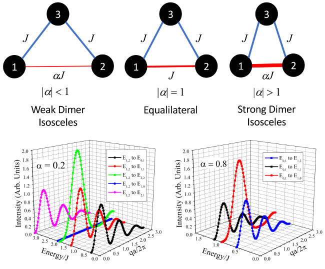
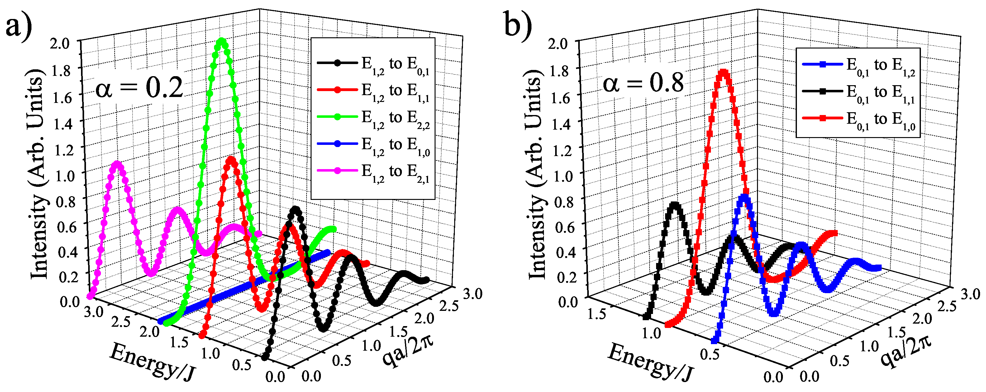
Figure 4S${}_t$ = 1 isosceles trimer single-crystal structure factors as a function of E/J vs. qa/$\pi$ with S${}_t$ = 1 ground state at $\alpha$ = 0.2 (a) and with S${}_t$ = 0 ground state at $\alpha$ = 0.8(b). Here, $r_{12}$ = $r_{13}$/2 = $r_{23}$/2 = a, where a is the spatial distance of the dimer. We also include a generic magnetic form factor to illustrate the damping effect that will be expressed at larger q [40]. Overall, the different structure factor functions allow for experimentalists to easily distinguish between dimer and trimer excitations, as well as extract geometric parameters through a fitting of the intensity profile.

Another point of interest is the change in ground state at $\alpha$ = 0.5, which brings a discontinuity to the neutron scattering intensities and helps to clarify the spin states of the ions. 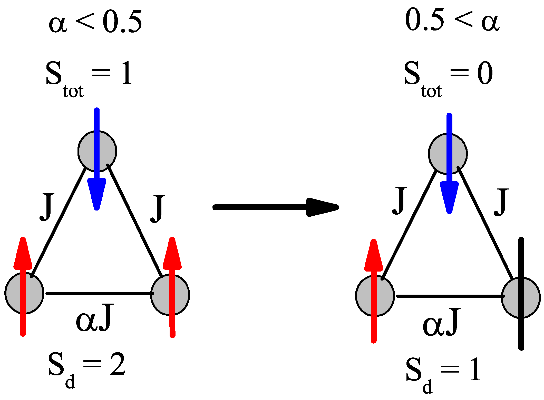The sudden change from a S${}_t$ = 0 to a S${}_t$ = 1 ground state in the S = 1 trimer immediately allows two more transitions that are described in Figure 4, where at $\alpha$ = 0.8 there are only three possible transitions and at $\alpha$ = 0.2 there are five possible transitions. As $\alpha$ decreases below 0.5 for the S = 1 case, the trimer is allowed to order itself into a less frustrated state with an overall spin of 1, but a dimer spin state of 2 (both ions are in spin up states. Whereas with $\alpha$ > 0.5, the trimer experiences a greater frustration that pushes the spins into a S${}_d$ = 1 dimer state (one spin and one neutral), which means the overall spin of the trimer is zero. This transition is illustrated in Figure 5. The S = 3/2 trimer has an analogous state flip at $\alpha$ = 0.5. The use of the spin dimer basis states therefore allows for the spin configurations to be known and a better understanding of the frustration of the trimer becomes clear. The nature of the change in ground state can be attributed to a change in the dimer basis.

Furthermore, an analysis of the inelastic neutron scattering structure factors reveals a hidden selection rule for magnetic clusters and molecular magnets. From Table 2, some of the transitions have no structure factor or inelastic scattering intensity, even though they have the standard neutron scattering transition of $\mathsf{\Delta }{S}_t$ = ±1 or 0. This zero intensity is due to the transition of the dimer being greater than ±1. This therefore clarifies the selection rule for magnetic clusters by extending it to the individual subgeometries.

5. Conclusions

We have presented calculations of the thermodynamics, inelastic neutron scattering excitations, and structure factors for general isosceles trimers. Using a Heisenberg spin-spin exchange model, we determined general relationships for the quantum energy levels, spin states, and spin decomposition of isosceles trimers for any spin. Through a calculation of the partition function, we determined the heat capacity and magnetic susceptibility as functions of temperature and dimer exchange coupling ($\alpha$). An analysis of the thermodynamics revealed multiple quantum phase transitions, where the temperature dependence of the Schottky anomaly indicated the proximity to this transition in $\alpha$. These transitions provided the potential for active spin switching in molecular clusters through a dynamic transition from external fields.

Furthermore, we examined the calculated neutron scattering structure factors (scattering intensities) for various excitations and showed that the spin total transitions did not just govern molecular magnet excitations, but the spin transition of the individual subgeometries. INS has a typical selection rule for magnetic states of $\mathsf{\Delta }$S = ±1 or 0, which means that neutron scattering will only examine transitions that are of a small spin variation. We presented here that the selection rules of neutron scattering of finite clusters should include another selection rule that is $\mathsf{\Delta }{S}_d$ = ±1 or 0, where $\mathsf{\Delta }{S}_d$ is that of that spin dimer basis. Because each spin state has a specific dimer basis associated with it, the different states are also bound by that basis. For example, the spin-1 equilateral trimer has three S = 1 excited states and two S = 2 excited states. Under standard INS selection rules, the transition from any of the S = 1 to the two S = 2 excited states is allowed. When the structure factors for these transitions are calculated, however, it becomes evident that not all the transitions are allowed. When examined closer, the S = 1 excited states have dimer bases of S${}_d$ = 0, 1, 2, and the S = 2 excited states have dimer bases of S${}_d$ = 1, 2.

Overall, the examination of spin trimers helps to provide insights into the foundational characteristics of molecular magnets. Through an understanding of the individual excitations of smaller clusters, one can determine the properties of larger, more complex clusters, which can help in the determination and realization of new and exciting spintronic materials and device applications.

In this model, we examined the isotropic Heisenberg Hamiltonian and the standard interactions to show the variation as spin evolves. Further studies could include other interactions and parameters (e.g., anisotropy, external magnetic field, biquadratic term, etc.) to examine the effect on the quantum phase transitions and the excitations that occur. Overall, these other terms should not have any impact on the functional form of the INS structure factors. Although, parameters like the external magnetic field will produce a Zeeman splitting of the excitations and anisotropy may shift the overall ground states. Further comprehensive studies can examine these effects.