Quasicrystal Tilings in Three Dimensions and Their Empires

Abstract

The projection method for constructing quasiperiodic tilings from a higher dimensional lattice provides a useful context for computing a quasicrystal’s vertex configurations, frequencies, and empires (forced tiles). We review the projection method within the framework of the dual relationship between the Delaunay and Voronoi cell complexes of the lattice being projected. We describe a new method for calculating empires (forced tiles) which also borrows from the dualisation formalism and which generalizes to tilings generated projections of non-cubic lattices. These techniques were used to compute the vertex configurations, frequencies and empires of icosahedral quasicrystals obtained as a projections of the $D_6$ and ${\mathbb{Z}}^6$ lattices to ${\mathbb{R}}^3$ and we present our analyses. We discuss the implications of this new generalization.

1. Introduction

Quasicrystals, since their discovery [1], had been an active area of research in mathematics, physics, chemistry and mineralogy. They have intriguing and complex structure which lies between disorder and periodicity and which exhibits several physical properties [2]. The mathematics describing aperiodic tilings come from a variety of methodologies [3,4,5] which give ideal geometries that model quasicrystalline structure on a global (infinite) scale.

Physically, quasicrystals are formed in materials via the local growth patterns of atoms as they anneal and coalesce. The atomic configurations are dictated by the geometry of the neighboring chemical bonds and the growth patterns are determined by how these configurations join together. A quasicrystal growing from a local configuration can benefit (have less defects) if there is a lower variability in possible growth patterns, that is, if more of the structure surrounding the site is forced [6,7]. Mathematically, the question regarding what portions of a quasicrystal are forced by an initial configuration is called the empire problem [8].

Previous research on the subject has been carried out by several authors using different approaches. One method is specific to the decorated Penrose tilings and uses Ammann bars in order to derive forced tiles [9,10]. Another method uses the multigrid formalism and introduces linear constraints imposed by tiles on the shift parameter to calculate empires [11]. Most recently, a method investigated by Fang et al. [12], is set in the context of the projection method and involves modifying [13] the cut-window in order to form a smaller empire window which serves as the acceptance domain for the empire of a specified patch of tiles. The latter construction is the more general of the three methods and has been used successfully to compute empires for several tilings generated as projections of cubic lattices ${\mathbb{Z}}^N\to {\mathbb{E}}^n$ [12].

In this paper, we present a new way of calculating empires which generalizes to quasiperiodic tilings derived as projections of non-cubic lattices. This method is also set within the framework of the cut-and-project formalism and relies on the dualisation of a lattice’s Voronoi and Delaunay complexes as prescribed by the Klotz construction [5].

In Section 2 we provide an overview of the projection method in the context of the dualisation formalism and introduce the cut-window along with its regions and sectors which serve as acceptance domains for vertices, tiles, and vertex configurations, respectively. In Section 3 we describe how sectors are used to compute vertex frequencies and present calculated results of the frequencies and sectors for each of the 36 vertex configurations of an icosahedral tiling, ${\mathcal{T}}^{(D_6)}$, defined a projection of the $D_6$ lattice to ${\mathbb{E}}^3$ [14,15,16]. In Section 4 we introduce our new method for computing empires and present empires calculated for vertex configurations of ${\mathcal{T}}^{(D_6)}$ as well as a tiling of Ammann [17] defined as a projection ${\mathbb{Z}}^6\to {\mathbb{E}}^3$.

2. Projection Method

In this section we summarize the projection method for generating quasiperiodic tilings. We first outline the selection process for vertices and introduce the cut-window. We demonstrate why more information is needed when determining tiles for projections of non-cubic lattices. Finally, we describe the projection method within the framework of the dualisation formalism between a lattice’s Voronoi and Delaunay cell complexes [3,14,15].

2.1. Overview of Projection Method

The projection method for constructing quasicrystals is characterized by a lattice $\mathsf{\Lambda }\subset {\mathbb{E}}^N$ along with projections ${\pi }_{\parallel } \mathrm{and} {\pi }_{\perp }$ onto orthogonal subspaces ${\mathbb{E}}_{\parallel } \mathrm{and} {\mathbb{E}}_{\perp }$. A convex volume $\mathcal{W}$ in the perpendicular space ${\mathbb{E}}_{\perp }$ called the cut-window acts as an acceptance domain for determining which points $\lambda \in \mathsf{\Lambda }$ are selected to have their projections ${\lambda }_{\parallel }$ included in the tiling $\mathcal{T}$ of ${\mathbb{E}}_{\parallel }$. For cubic lattices ($\mathsf{\Lambda }={\mathbb{Z}}^N$) the cut-window is sufficient for determining which tiles fill the tiling space ${\mathbb{E}}_{\parallel }$. But when projecting non-cubic lattices, the proper selection of tiles is more nuanced and requires that the cut-window be subdivided into regions which act as acceptance domains for individual tiles types. These regions can be further subdivided into sectors which serve as acceptance domains for specific vertex configurations; computing the relative sector volumes gives the vertex frequencies. Furthermore, similar constructions involving the regions of the cut-window can be used to compute empires in a concise and novel way.

Let $\mathsf{\Lambda }$ be a regular point lattice in an N-dimensional Euclidean space, ${\mathbb{E}}^N$, which is defined as the integer combinations of some finite set of lattice root vectors $v_i$:

$$\mathsf{\Lambda }=\{a_1{v}_1+\cdots +a_k{v}_k:a_i\in \mathbb{Z},v_i\in {\mathbb{E}}^N\}.$$

(1)

It is assumed [5] that the vectors $v_i$ span all of ${\mathbb{E}}^N$, and that the convex hull of the lattice itself is the entire space, $\mathrm{conv}(\mathsf{\Lambda })={\mathbb{E}}^N$. Also, we assume that the lattice is a discrete point set, meaning that it has no accumulation points in ${\mathbb{E}}^N$. Let ${\mathbb{E}}_{\parallel }$ be an n-dimensional affine subspace of ${\mathbb{E}}^N$ in which a space-filling tiling $\mathcal{T}$ will be constructed. For the purpose of creating an aperiodic tiling in ${\mathbb{E}}_{\parallel }$, it is necessary for ${\mathbb{E}}_{\parallel }$ to lie at irrational angles to the vectors which generate the lattice. Let ${\mathbb{E}}_{\perp }$ be the orthogonal complement to ${\mathbb{E}}_{\parallel }$ and let ${\pi }_{\parallel }$ and ${\pi }_{\perp }$ denote the projections onto ${\mathbb{E}}_{\parallel }$ and ${\mathbb{E}}_{\perp }$, respectively.

The projection method dictates that a lattice point $\lambda \in \mathsf{\Lambda }$ will be included in the tiling $\mathcal{T}$ precisely when the tiling subspace ${\mathbb{E}}_{\parallel }$ intersects non-trivially with the Voronoi cell $V(\lambda )$ containing $\lambda$ [5]:

$$\lambda \in \mathcal{T}\iff V\left(\lambda \right)\cap {\mathbb{E}}_{\parallel }\ne \varnothing ,$$

(2)

where the Voronoi cell of a lattice point $V\left(\lambda \right)$ is the convex region in ${\mathbb{E}}^N$ defined relative to the lattice by:

$$V\left(\lambda \right)=\{x\in {\mathbb{E}}^N:|x-\lambda |\le |x-{\lambda }^{\prime }|, \forall {\lambda }^{\prime }\in \mathsf{\Lambda }\}.$$

(3)

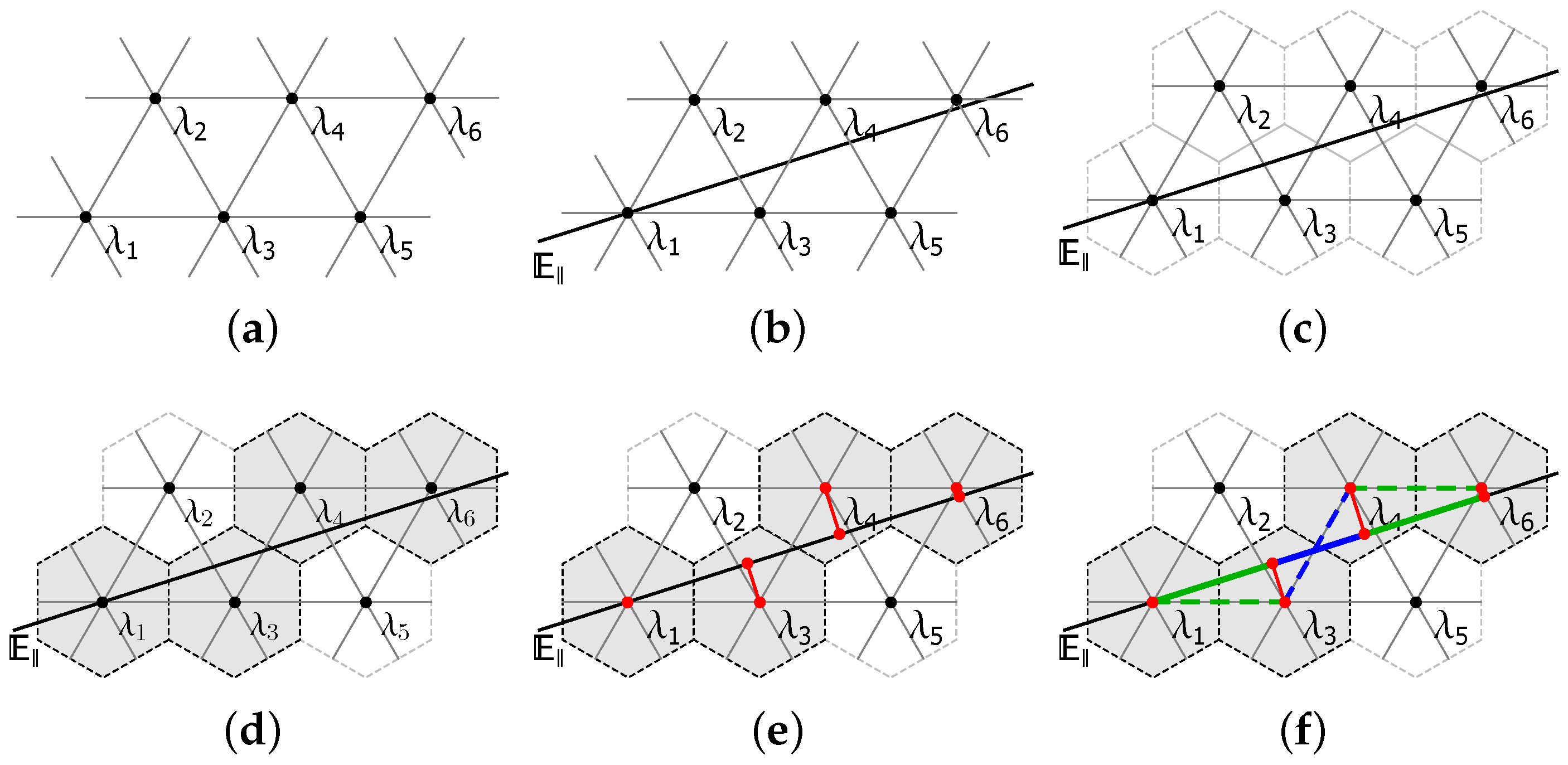
See Figure 1 for an example of the selection process defined by Equation (2) for a quasicrystal tiling, denoted ${\mathcal{T}}^{(A_2)}$, defined as a projection of the triangular $A_2$ lattice to ${\mathbb{R}}^1$. This selection criteria determines which vertices $\lambda$ are included in the tiling $\mathcal{T}$. The next step is to understand how the selected vertices are connected by edges, faces, …, and k-polytopes. The polytopes of $\mathcal{T}$ are selected from the polytopes of the Delaunay complex of the lattice. The polytopes which become the proper space-filling tiles $\mathbf{t}$ covering ${\mathbb{E}}_{\parallel }$ are n-dimensional polytopes of the lattice’s Delaunay complex which project to n-dimensional polytopes in ${\mathbb{E}}_{\parallel }$. In order for such a polytope $\mathbf{t}=\mathrm{conv}\{{\lambda }_1,\dots ,{\lambda }_k\}$ to be included in the tiling $\mathcal{T}$, it is certainly necessary that each of its vertices be included in $\mathcal{T}$ as well (i.e., $V({\lambda }_i)\cap {\mathbb{E}}_{\parallel }\ne \varnothing$). 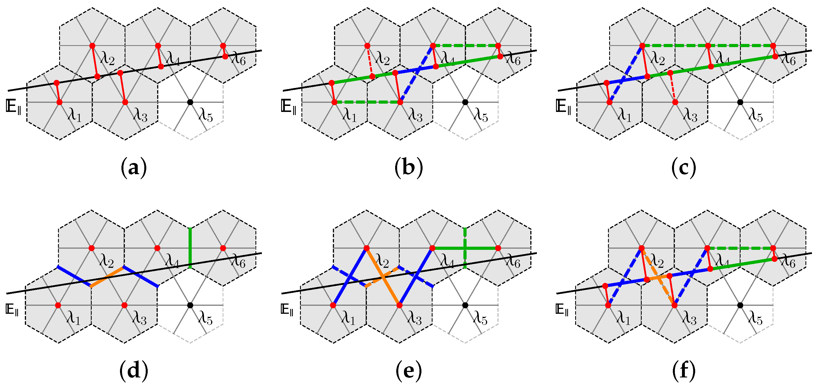This condition is necessary, and for cubic lattices it suffices to yield an accurate selection of tiles. But when projecting from a non-cubic lattice, these criteria are insufficient and in some cases can lead to an inconsistent selection of tiles (e.g., tiles that overlap or otherwise intersect). See Figure 2 for a scenario (in the case of a projection $A_2\to {\mathbb{E}}^1$) where following this rule alone leads to overlapping tiles in ${\mathbb{E}}_{\parallel }$.

Figure 1. Step-by-step illustration of the cut-and-project process for the triangular lattice $\mathsf{\Lambda }=A_2$ (a) projecting onto a 1-dimensional tiling space ${\mathbb{E}}_{\parallel }$ (b). The Voronoi cells for the lattice are all regular hexagons (c) and it is only those vertices with Voronoi cells that intersect ${\mathbb{E}}_{\parallel }$ which are selected (d). These vertices are then projected onto ${\mathbb{E}}_{\parallel }$ and define the vertices of the tiling of ${\mathbb{E}}_{\parallel }$ (e). The lattice edges (dashed lines) connecting the selected lattice points are projected to ${\mathbb{E}}_{\parallel }$ to form the (1-dimensional) tiles which fill ${\mathbb{E}}_{\parallel }$ (f).

Figure 2. A cut and projection $A_2\to {\mathbb{E}}^1$, where ${\mathbb{E}}_{\parallel }$ has a shallow enough slope that overlapping edges can arise when one is deciding which edges to select as tiles. (a) The space ${\mathbb{E}}_{\parallel }$ intersects the Voronoi cells of lattices points ${\lambda }_i$ for $i=\{1,2,3,4,6\}$. It is not clear, however, which edges should be selected as tiles in ${\mathbb{E}}_{\parallel }$. For instance (b) the edge from ${\lambda }_1^{\parallel }$ to ${\lambda }_3^{\parallel }$ clashes with the vertex ${\lambda }_2^{\parallel }$ and similarly (c) the edge connecting ${\lambda }_2^{\parallel }$ to ${\lambda }_4^{\parallel }$ conflicts with the vertex ${\lambda }_3^{\parallel }$. The solution lies with the boundary facets of the Voronoi cells. Each lattice edge $\{{\lambda }_a,{\lambda }_b\}$ is dual to the facet that forms the common boundary between $V({\lambda }_a)$ and $V({\lambda }_b)$. It is only when ${\mathbb{E}}_{\parallel }$ intersects with the boundary facet $V({\lambda }_a)\cap V({\lambda }_b)$ that the edge $\{{\lambda }_a^{\parallel },{\lambda }_b^{\parallel }\}$ is selected for the tiling. The boundary facets which intersect ${\mathbb{E}}_{\parallel }$ (d) and the edges to which they are dual (e) are the correct choice of edges which project to ${\mathbb{E}}_{\parallel }$ without overlapping (f).

Before giving the condition for properly selecting which edges to project to ${\mathbb{E}}_{\parallel }$ for inclusion in the tiling $\mathcal{T}$, we first take a moment to talk about the polytopes which comprise the Voronoi cells themselves. This has investigated in detail by previous authors [5,18], so here we provide only an overview. The Voronoi cells are convex polytopes which tessellate and fill the space ${\mathbb{E}}^N$. These polytopes have boundary facets which are themselves convex polytopes (of co-dimension 1), and which themselves have boundaries (of co-dimension 2), and so on.

Let $\mathcal{V}$ denote the Voronoi complex defined (relative to the lattice) as the set of all the Voronoi cells $V(\lambda )$ along with all of their boundary polytopes:

$$\mathcal{V}:=\{P\subset V(\lambda ):P \mathrm{is} \mathrm{a} \mathrm{boundary} \mathrm{of} V(\lambda ) \mathrm{for} \mathrm{some} \lambda \in \mathsf{\Lambda }\}.$$

(4)

It should be noted that the Voronoi cells themselves, being volumetric N-cells in ${\mathbb{E}}^N$, are also considered as ‘boundaries’ and are included in $\mathcal{V}$. The Voronoi cells are situated in face-to-face relation so the set $\mathcal{V}$ is a proper honeycomb in ${\mathbb{E}}^N$ and exhibits properties similar to that of a simplicial complex [5]:

$$\begin{array}{c}\mathrm{If} P_1\in \mathcal{V} \mathrm{and} P_2 \mathrm{is} \mathrm{a} \mathrm{boundary} \mathrm{of} P_1, \mathrm{then} P_2\in \mathcal{V}.\hfill \end{array}$$

(5)

$$\begin{array}{c}\mathrm{If} P_2,P_2\in \mathcal{V} \mathrm{and} (P_1\cap P_2)\ne \varnothing , \mathrm{then} (P_1\cap P_2) \mathrm{is} \mathrm{also} \mathrm{a} \mathrm{boundary} \mathrm{in} \mathcal{V}.\hfill \end{array}$$

(6)

The dual to the Voronoi complex is the Delaunay complex ${\mathcal{V}}^{\ast }$ which also exhibits properties (5) and (6). The Delaunay complex ${\mathcal{V}}^{\ast }$ has as its vertices precisely the lattice points $\mathsf{\Lambda }$. The n-cells ${\mathbf{t}}^n$ of ${\mathcal{V}}^{\ast }$ are the polytopes from which the tiles of $\mathcal{T}$ are selected and projected to ${\mathbb{E}}_{\parallel }^n$. The regularity of the lattice ensures that the Voronoi domains form a regular tessellation of ${\mathbb{E}}^N$, and the polytopes of $\mathcal{V}$ are translated copies of the set of polytopes which comprise the (generic) Voronoi polytope at the origin, $V=V(\overrightarrow{0})$. So the polytopes of $\mathcal{V}$ can be categorized by computing the cell decomposition of the single polytope: $V$. Similarly, the polytopes of ${\mathcal{V}}^{\ast }$ can be seen as translated copies of just those polytopes that are dual to the polytopes of $V$, which are precisely the polytopes of the Delaunay complex that are adjacent to the origin. The dual correspondence between $\mathcal{V}$ and ${\mathcal{V}}^{\ast }$ is given as follows:

$$\begin{array}{ccc}\hfill P\in \mathcal{V},& P^{\ast }:=& \mathrm{conv}\{\lambda \in \mathsf{\Lambda }:V(\lambda ) \mathrm{contains} P \mathrm{as} \mathrm{a} \mathrm{boundary}\},\hfill \end{array}$$

(7)

$$\begin{array}{ccc}\hfill Q\in {\mathcal{V}}^{\ast },& Q^{\ast }:=& \bigcap _{\lambda \in Q}V(\lambda ).\hfill \end{array}$$

(8)

Individual lattice points (0-polytopes), ${\mathbf{t}}^0=\{\lambda \}$, are dual to their respective Voronoi N-cells ${\{\lambda \}}^{\ast }=V\left(\lambda \right)$. An edge (1-polytope) inscribed between neighboring lattice points, ${\mathbf{t}}^1=\mathrm{conv}\{{\lambda }_1,{\lambda }_2\}$, is dual to the $(N-1)$-facet which their Voronoi domains both share at their intersection $\mathrm{conv}{\{{\lambda }_1,{\lambda }_2\}}^{\ast }=V({\lambda }_1)\cap V({\lambda }_2)$. In general, a k-polytope ${\mathbf{t}}^k=\mathrm{conv}\{{\lambda }_1,\dots ,{\lambda }_l\}\in {\mathcal{V}}^{\ast }$ will be dual to the polytope that lies at the common intersection of all the lattice points’ Voronoi domains, ${\mathbf{t}}^{\ast }={\bigcap }_{i}V({\lambda }_i)$. In all cases, a polytope and its dual are always orthogonal to each other, $\mathbf{t}\perp {\mathbf{t}}^{\ast }$, and their dimensions are always complementary in ${\mathbb{E}}^N$, $\dim (\mathbf{t})+\dim ({\mathbf{t}}^{\ast })=N$.

It is in this context of this dualisation formalism that we give the criteria for selecting which polytopes are included in the tiling. The tiles $\mathbf{t}$ of $\mathcal{T}$ are selected among the n-dimensional polytopes of ${\mathcal{V}}^{\ast }$. An n-polytope $\mathbf{t}\in {\mathcal{V}}^{\ast }$ is selected for the tiling if its dual polytope ${\mathbf{t}}^{\ast }$ intersects non-trivially with the tiling space ${\mathbb{E}}_{\parallel }$. Also, we are interested in only those polytopes which have non-degenerate projections to ${\mathbb{E}}_{\parallel }$ [18]. It is in this regard that we give the definition for the tiling $\mathcal{T}$:

$$\mathcal{T}=\{\mathbf{t}\in {\mathcal{V}}^{\ast }:\dim (\mathbf{t})=n=\dim ({\mathbf{t}}_{\parallel }),{\mathbf{t}}^{\ast }\cap {\mathbb{E}}_{\parallel }\ne \varnothing \}.$$

(9)

2.2. Lattice Points and the Cut-Window

For a regular lattice, the Voronoi cells are identical up to translation, satisfying $V\left(\lambda \right)=(V+\lambda )$. The condition $V\left(\lambda \right)\cap {\mathbb{E}}_{\parallel }\ne \varnothing$ is equivalent to there being some point $x\in (V+\lambda )$ where $x\in {\mathbb{E}}_{\parallel }$, or rather, $(x-\lambda )\in V$. Taking the projection under ${\pi }_{\perp }$, we have $(x_{\perp }-{\lambda }_{\perp })\in V_{\perp }$, but $x_{\perp }=\overrightarrow{0}$ (since $x\in {\mathbb{E}}_{\parallel }$) which gives $-{\lambda }_{\perp }\in V_{\perp }$, or simply: ${\lambda }_{\perp }\in -V_{\perp }$. The regularity of the lattice comes into play again, giving the symmetry $V=-V$, so the final condition is just ${\lambda }_{\perp }\in V_{\perp }$. The projected image $V_{\perp }\subset {\mathbb{E}}_{\parallel }$ is called the cut-window, denoted by $\mathcal{W}$, and it plays a central role in both the construction and analysis of the tilings generated via the projection method.

Determining if a lattice point $\lambda$ is to be included in the tiling, ${\lambda }_{\parallel }\in \mathcal{T}$, reduces to finding out if that lattice point’s orthogonal projection ${\lambda }_{\perp }$ falls within the fixed convex volume in ${\mathbb{E}}_{\perp }$ given by the cut-window $\mathcal{W}=V_{\perp }$:

$${\lambda }_{\parallel }\in \mathcal{T}\iff {\lambda }_{\perp }\in \mathcal{W}.$$

(10)

In Figure 3, the cut-window is depicted for a quasicrystal tiling ${\mathcal{T}}^{(A_2)}$ projection $A_2\to {\mathbb{R}}^1$ in which the Voronoi domains are hexagons and the cut-window is an interval in ${\mathbb{E}}_{\perp }$ defined by the total width of a hexagon’s projection to ${\mathbb{E}}_{\parallel }$.

Figure 3. A tiling ${\mathcal{T}}^{(A_2)}$ defined as a projection $A_2\to {\mathbb{E}}^1$ of the triangular lattice to the line. The cut-window $\mathcal{W}=V_{\perp }$ is an interval in ${\mathbb{E}}_{\perp }$ (thick red line) and dictates which lattice points $\lambda$ are selected for the tiling $\mathcal{T}$: if a lattice points falls within the cut-window ${\lambda }_{\perp }\in \mathcal{W}$ then it is included in the tiling $\lambda \in \mathcal{T}$.

2.3. Tiles and Regions of the Cut-Window

The regularity of lattice allows us to characterize all tiles $\mathbf{t}\in {\mathcal{V}}^{\ast }$ using a finite set of tile types, $\tilde{\mathbf{t}}$, which are just those tiles of ${\mathcal{V}}^{\ast }$ which are adjacent to the origin. Each tile $\mathbf{t}\subset {\mathbb{E}}^N$ can be expressed as a translation of one of the tile types: for any $\lambda \in \mathbf{t}$, $\mathbf{t}=\tilde{\mathbf{t}}+\lambda$ where $\tilde{\mathbf{t}}=(\mathbf{t}-\lambda )$ is a tile containing the origin. The dual to a tile can then be expressed as a translation of the dual of some tile type: ${\mathbf{t}}^{\ast }={(\tilde{\mathbf{t}}+\lambda )}^{\ast }=({\tilde{\mathbf{t}}}^{\ast }+\lambda )$. For $\mathbf{t}\in \mathcal{T}$ to be included in a tiling, it is necessary that ${\mathbf{t}}^{\ast }$ intersects non-trivially with ${\mathbb{E}}_{\parallel }$, which can be written as $({\tilde{\mathbf{t}}}^{\ast }+\lambda )\cap {\mathbb{E}}_{\parallel }\ne \varnothing$. Supposing $\overrightarrow{x}\in ({\tilde{\mathbf{t}}}^{\ast }+\lambda )\cap {\mathbb{E}}_{\parallel }$, we take the projection to ${\mathbb{E}}_{\perp }$ and find ${\overrightarrow{x}}_{\perp }\in {({\tilde{\mathbf{t}}}^{\ast }+\lambda )}_{\perp }$ which gives $\overrightarrow{0}\in ({\tilde{\mathbf{t}}}_{\perp }^{\ast }+{\lambda }_{\perp })$ or simply: ${\lambda }_{\perp }\in -{\tilde{\mathbf{t}}}_{\perp }^{\ast }$.

The volumes $\mathfrak{r}=(-{\tilde{\mathbf{t}}}_{\perp }^{\ast })\subset \mathcal{W}$ are called regions of the cut-window. The regions are in direct correspondence to the tile types and each region serves as an acceptance domain for its respective tile type (see Figure 4) in the following way: for a region $\mathfrak{r}=-{\tilde{\mathbf{t}}}_{\perp }^{\ast }$, if a lattice point $\lambda$ has a projection ${\lambda }_{\perp }$ that lands within $\mathfrak{r}$, ${\lambda }_{\perp }\in \mathfrak{r}$, then the tile $\mathbf{t}=(\tilde{\mathbf{t}}+\lambda )$ will be a valid tile in $\mathcal{T}$.

Figure 4. (a–c) Three of the six tile types $\tilde{\mathbf{t}}$ (colored arrows) are shown for the ${\mathcal{T}}^{(A_2)}$ along with their corresponding regions $\mathfrak{r}=-{\tilde{\mathbf{t}}}_{\perp }^{\ast }\subset \mathcal{W}$ (thick red lines). Any lattice point $\lambda$ which falls into a region, ${\lambda }_{\perp }\in \mathfrak{r}$, will be adjacent to a tile $\mathbf{t}$ which is a translated copy $\mathbf{t}=(\tilde{\mathbf{t}}+\lambda )$ of the tile type $\tilde{\mathbf{t}}$ corresponding to $\mathfrak{r}$. (d) The selected tiles are shown along with the whole cut-window.

It should be noted that it is only those regions $\mathfrak{r}=-{\tilde{\mathbf{t}}}_{\perp }^{\ast }$ which are proper $(N-n)$-dimensional volumes in $\mathcal{W}$ that are useful in selecting the proper (space-filling) tiles of ${\mathbb{E}}_{\parallel }$. If a region is degenerate, that is if $\dim ({\tilde{\mathbf{t}}}_{\perp }^{\ast })<(N-n)$ inside ${\mathbb{E}}_{\perp }$, then $\dim ({\tilde{\mathbf{t}}}_{\parallel })<n$ inside ${\mathbb{E}}_{\parallel }$ and $\mathbf{t}=(\mathbf{t}+\lambda )$ cannot be included in $\mathcal{T}$ as $\dim ({\mathbf{t}}_{\parallel })<n$ meaning ${\mathbf{t}}_{\parallel }$ cannot be a space-filling tile of ${\mathbb{E}}_{\parallel }$. In this regard, we may redefine the tiling in the following way:

$$\mathcal{T}=\{\mathbf{t}=(\tilde{\mathbf{t}}+\lambda ):{\lambda }_{\perp }\in \mathfrak{r} \mathrm{where} \mathfrak{r}=-{\tilde{\mathbf{t}}}_{\perp }^{\ast }\}.$$

(11)

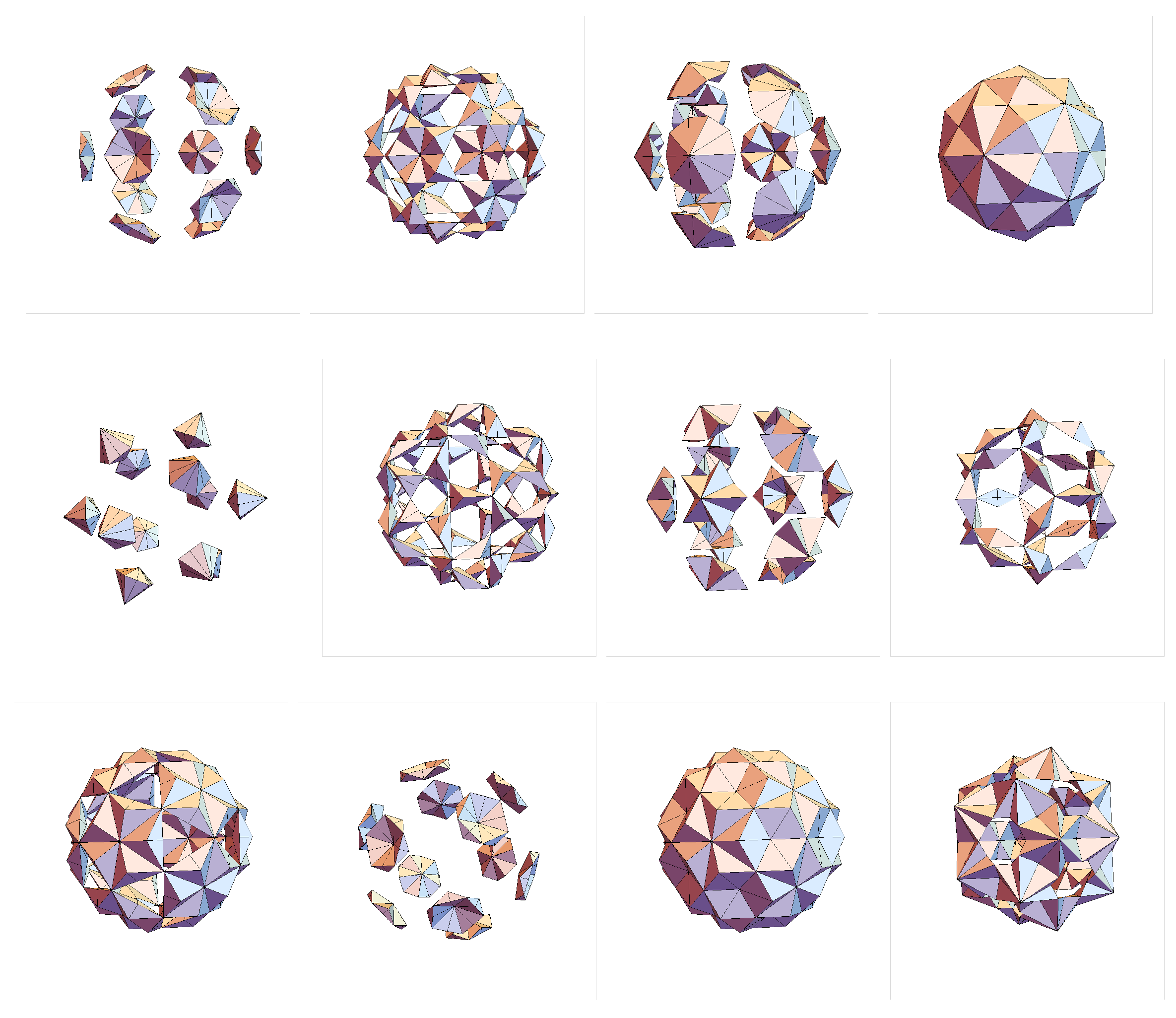
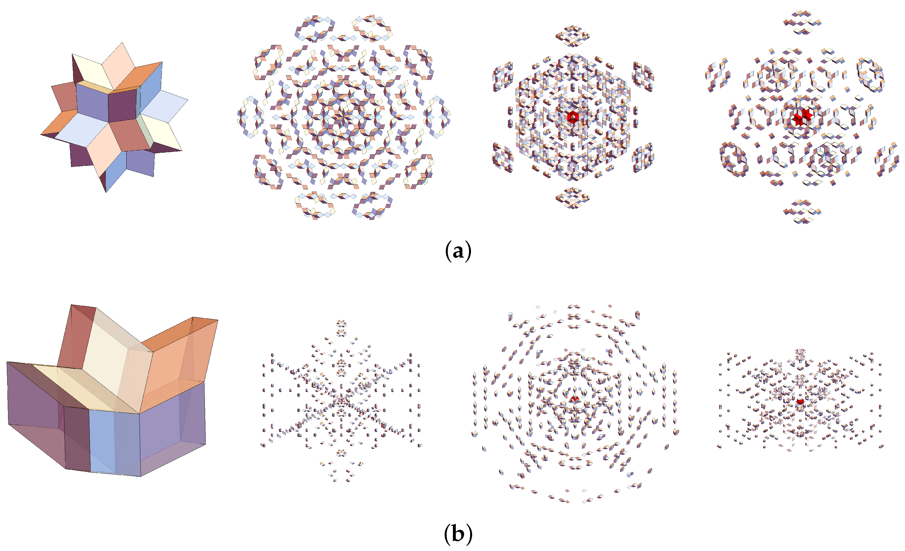
It should be noted that the cut-window regions may be quite different than the tiles to which they correspond. In the case of the tiling ${\mathcal{T}}^{(D_6)}$ (Figure 5) defined by a certain projection of the lattice $\mathsf{\Lambda }=D_6$ to ${\mathbb{R}}^3$, the Voronoi cell is a 6-dimensional polytope that has as its 3-dimensional boundaries 960 pyramids (with rhombus bases) and 160 rhombohedrons (parallelepipeds) [18], (see Figure 6). The duals to these pyramids and rhombohedrons are 1120 regular tetrahedrons in ${\mathbb{E}}^6$ whose vertices are lattice points $\lambda \in D_6$. The tetrahedrons are distorted in the projection to ${\mathbb{E}}_{\parallel }$ (their images are no longer regular) and 240 of them are degenerate in the projection to ${\mathbb{E}}_{\perp }$ leaving 880 non-degenerate regions of $\mathcal{W}$ corresponding to 880 non-degenerate tiles types for ${\mathcal{T}}^{(D_6)}$.

Figure 5. Various tilings ${\mathcal{T}}^{(D_6)}$ generated as projections $D_6\to {\mathbb{E}}^3$ with randomly chosen shift vectors.

Figure 6. Tiles and corresponding cut-window regions for the tiling ${\mathcal{T}}^{(D_6)}$. Four tiles are shown (left) alongside their corresponding regions (right) in the cut-window. The tiles ${\mathcal{T}}^{(D_6)}$ are all tetrahedrons while their corresponding regions are pyramids with a rhombic base (a–c) or parallelepipeds (d).

2.4. Vertex Configurations and Sectors of $\mathcal{W}$

For a lattice point $\lambda \in \mathcal{T}$, its vertex configuration $\mathfrak{C}\left(\lambda \right)$ is defined to be the set of tiles that are adjacent to it:

$$\mathfrak{C}\left(\lambda \right):=\{\mathbf{t}\in \mathcal{T}:\lambda \in \mathbf{t}\}.$$

(12)

Because each tile $\mathbf{t}=(\tilde{\mathbf{t}}+\lambda )$ corresponds to a region $\mathfrak{r}=-{\tilde{\mathbf{t}}}_{\perp }^{\ast }$, the vertex configuration for a lattice point $\mathfrak{C}\left(\lambda \right)$ can be derived by taking the tiles associated with those regions of the cut-window which contain ${\lambda }_{\perp }$:

$$\mathfrak{C}(\lambda ):=\{(\tilde{\mathbf{t}}+\lambda )\in \mathcal{T}:{\lambda }_{\perp }\in \mathfrak{r}, \mathfrak{r}=-{\tilde{\mathbf{t}}}_{\perp }^{\ast }\}.$$

(13)

The mutual intersection of all the regions which contain ${\lambda }_{\perp }$ defines a certain sector, $\mathfrak{s}$, a volume inside the cut-window which corresponds to the vertex configuration $\mathfrak{C}\left(\lambda \right)$ associated with $\lambda$.

$$\mathfrak{s}\left(\lambda \right):=\bigcap _{{\lambda }_{\perp }\in \mathfrak{r}}\mathfrak{r}.$$

(14)

Any other lattice point ${\lambda }^{\prime }$ whose projection ${\lambda }_{\perp }^{\prime }$ falls within the same sector $\mathfrak{s}\left(\lambda \right)$ will have an identical vertex configuration to $\lambda$, since by definition $\lambda$ and ${\lambda }^{\prime }$ are adjacent to the same types of tiles. See Figure 7 for an example vertex configuration and corresponding sector for the ${\mathcal{T}}^{(A_2)}$ tiling.

Figure 7. A vertex configuration $\tilde{\mathfrak{C}}$ (the combination of blue and green tile types) and its corresponding sector $\mathfrak{s}\subset {\mathbb{E}}_{\perp }$ (red) for the ${\mathcal{T}}^{(A_2)}$ tiling. Two tile types $\tilde{\mathbf{t}}$ (blue arrow) and ${\tilde{\mathbf{t}}}^{\prime }$ (green arrow) together make up the vertex configuration $\tilde{\mathfrak{C}}=\{\tilde{\mathbf{t}},{\tilde{\mathbf{t}}}^{\prime }\}$. Their corresponding regions in the cut-window, $\mathfrak{r}=-{\mathbf{t}}_{\perp }^{\ast }$ (thick blue) and ${\mathfrak{r}}^{\prime }=-{{\mathbf{t}}^{\prime }}_{\perp }^{\ast }$ (thick green) overlap in $\mathcal{W}$ and their intersection $\mathfrak{s}=\mathfrak{r}\cap {\mathfrak{r}}^{\prime }$ is the sector which corresponds to the configuration defined by the two tile types. A lattice point $\lambda$ which falls into this sector, ${\lambda }_{\perp }\in \mathfrak{s}$, will have a translated copy of $\tilde{\mathfrak{C}}$ as its vertex configuration, $\mathfrak{C}(\lambda )=\tilde{\mathfrak{C}}+\lambda$.

For the tiling ${\mathcal{T}}^{(D_6)}$ there are 880 pyramids and rhombohedrons which serve as the regions of the cut-window. Their intersections go on to form 4230 sectors, corresponding to the different vertex configurations of the tiling. There are 36 vertex configurations, and each one comes in 120 different orientations up to icosahedral symmetry in ${\mathbb{E}}_{\parallel }$ (except for one configuration which exhibits only distinct 30 orientations). This accounts for all of the 4230 sectors ($35\times 120+1\times 30=4230$), and when the sectors are grouped according to these 36 vertex configurations, the sectors are seen to exhibit the same icosahedral symmetry within the cut-window $\mathcal{W}\subset {\mathbb{E}}_{\perp }$ (see Figure 8).

Figure 8. Sectors corresponding to twelve of the 36 vertex types of the tiling ${\mathcal{T}}^{(D_6)}$ (projection $D_6\to {\mathbb{E}}^3$) are shown. Each vertex configuration comes in 120 orientations (respecting the $H_3$ symmetry present in ${\mathbb{E}}_{\parallel }$) and so each configuration corresponds to 120 individual sectors in $\mathcal{W}$. Each group of 120 sectors, in turn, exhibits the same $H_3$ symmetry in the cut-window $\mathcal{W}\subset {\mathbb{E}}_{\perp }$.

3. Frequencies of Vertex Configurations

The cut-window $\mathcal{W}$ is divided up into non-overlapping sectors $\mathfrak{s}$ which correspond to all the possible vertex configurations (in all possible orientations) that are found in the tiling $\mathcal{T}$. The volume of a given sector, $\mathrm{vol}\left(\mathfrak{s}\right)$, as measured relative to the volume of the cut-window $\mathcal{W}$ as a whole, $(\mathrm{vol}(\mathfrak{s})/\mathrm{vol}(\mathcal{W}))$, gives the probability that a lattice point falling in the cut-window (${\lambda }_{\perp }\in \mathcal{W}$) will have the region’s corresponding arrangement of tiles as its vertex configuration. It is in this context that we define the frequency, $\mathcal{F}(\mathfrak{C})$, of a vertex configuration as this ratio of volumes:

$$\mathcal{F}(\mathfrak{C}(\lambda )):=\frac{\mathrm{vol}(\mathfrak{s}(\lambda ))}{\mathrm{vol}(\mathcal{W})}.$$

(15)

Frequency analysis for vertex configurations have computed in the past for several quasicrystals including the Penrose tiling [19], the Danzer tiling [20], and others [18,21]. For this paper, we have calculated the vertex configurations and their corresponding sectors, empires, and frequencies for the tiling ${\mathcal{T}}^{(D_6)}$ (see Table 1). The same analysis has been carried out by Kramer et al. [18] for ${\mathcal{T}}^{(D_6)}$ (which they notate as ${\mathcal{T}}^{\ast (2F)}$) and in Table 2 we provide a comparison of our results with their data and give the correspondence between the two lists.

Table 1. The 36 vertex configurations $\mathfrak{C}$ for the tiling ${\mathcal{T}}^{(D_6)}$ are shown along with their corresponding cut-window sectors $\mathfrak{s}\left(\mathfrak{C}\right)$, their empires $\mathcal{E}\left(\mathfrak{C}\right)$, and their frequencies $\mathcal{F}\left(\mathfrak{C}\right)$.

$\mathfrak{C}$	$\mathfrak{S}(\mathfrak{C})$	$\mathcal{E}(\mathfrak{C})$	$\mathcal{F}(\mathfrak{C})$	$\mathfrak{C}$	$\mathfrak{S}(\mathfrak{C})$	$\mathcal{E}(\mathfrak{C})$	$\mathcal{F}(\mathfrak{C})$
			$-38+17\sqrt{5}$				$-360+161\sqrt{5}$
			$843-377\sqrt{5}$				$-521+233\sqrt{5}$
			$233\sqrt{5}-521$				$161-72\sqrt{5}$
			$322-144\sqrt{5}$				$233\sqrt{5}-521$
			$161-72\sqrt{5}$				$843-377\sqrt{5}$
			$161-72\sqrt{5}$				$47-21\sqrt{5}$
			$305\sqrt{5}-682$				$161-72\sqrt{5}$
			$17\sqrt{5}-38$				$123-55\sqrt{5}$
			$47-21\sqrt{5}$				$17\sqrt{5}-38$
			$17\sqrt{5}-38$				$17\sqrt{5}-38$
			$9-4\sqrt{5}$				$17\sqrt{5}-38$
			$89\sqrt{5}-199$				$322-144\sqrt{5}$
			$34\sqrt{5}-76$				$233\sqrt{5}-521$
			$161-72\sqrt{5}$				$17\sqrt{5}-38$
			$161-72\sqrt{5}$				$161-72\sqrt{5}$
			$18-8\sqrt{5}$				$-2+\sqrt{5}$
			$-38+17\sqrt{5}$				$9-4\sqrt{5}$
			$-11+5\sqrt{5}$				$9-4\sqrt{5}$

Table 2. Comparison of data computed for the ${\mathcal{T}}^{(D_6)}$ by authors and by Kramer et at. [18]. Here, $\tau =(1+\sqrt{5})/2$ is the Golden Ratio and the ambiguity between types 16.1 and 23.1 is notated.

$\mathfrak{C}$	$\mathfrak{S}\left(\mathfrak{C}\right)$	$\mathcal{F}\left(\mathfrak{C}\right)$	$\mathcal{F}\left(\mathfrak{C}\right)$ (Kramer et al.)	Type (Kramer et al.)
		$-38+17\sqrt{5}$	$\frac{1}{{\tau }^9}$	$24.1$
		$-360+161\sqrt{5}$	$\frac{1+{\tau }^2}{{\tau }^{13}}$	$14.1$
		$843-377\sqrt{5}$	$\frac{2}{{\tau }^{14}}$	$13.1$
		$-521+233\sqrt{5}$	$\frac{2}{{\tau }^{13}}$	$17.1$
		$-521+233\sqrt{5}$	$\frac{2}{{\tau }^{13}}$	$12.1$
		$161-72\sqrt{5}$	$\frac{1}{{\tau }^{12}}$	$20.1$
		$322-144\sqrt{5}$	$\frac{2}{{\tau }^{12}}$	$18.1$
		$-521+233\sqrt{5}$	$\frac{2}{{\tau }^{13}}$	$21.1$
		$161-72\sqrt{5}$	$\frac{1}{{\tau }^{12}}$	$16.1$ (or $23.1$)
		$843-377\sqrt{5}$	$\frac{2}{{\tau }^{14}}$	$19.1$
		$161-72\sqrt{5}$	$\frac{1}{{\tau }^{12}}$	$15.1$
		$47-21\sqrt{5}$	$\frac{2}{{\tau }^8}$	$11.4$
		$-682+305\sqrt{5}$	$\frac{1}{{\tau }^{15}}$	$22.1$
		$161-72\sqrt{5}$	$\frac{1}{{\tau }^{15}}$	$23.1$ (or $16.1$)
		$-38+17\sqrt{5}$	$\frac{1}{{\tau }^9}$	$11.1$
		$123-55\sqrt{5}$	$\frac{2}{{\tau }^{10}}$	$9.1$
		$47-21\sqrt{5}$	$\frac{2}{{\tau }^8}$	$9.3$
		$-38+17\sqrt{5}$	$\frac{1}{{\tau }^9}$	$2.2$
		$-38+17\sqrt{5}$	$\frac{1}{{\tau }^9}$	$10.4$
		$-38+17\sqrt{5}$	$\frac{1}{{\tau }^9}$	$1.2$
		$9-4\sqrt{5}$	$\frac{1}{{\tau }^6}$	$11.3$
		$-38+17\sqrt{5}$	$\frac{1}{{\tau }^9}$	$2.1$
		$-199+89\sqrt{5}$	$\frac{2}{{\tau }^{11}}$	$9.2$
		$322-144\sqrt{5}$	$\frac{2}{{\tau }^{12}}$	$5.1$
		$-76+34\sqrt{5}$	$\frac{2}{{\tau }^9}$	$10.1$
		$-521+233\sqrt{5}$	$\frac{2}{{\tau }^{13}}$	$3.1$
		$161-72\sqrt{5}$	$\frac{1}{{\tau }^{12}}$	$1.1$
		$-38+17\sqrt{5}$	$\frac{1}{{\tau }^9}$	$11.2$
		$161-72\sqrt{5}$	$\frac{1}{{\tau }^{12}}$	$4.1$
		$161-72\sqrt{5}$	$\frac{1}{{\tau }^{12}}$	$10.2$
		$18-8\sqrt{5}$	$\frac{2}{{\tau }^6}$	$11.5$
		$-2+\sqrt{5}$	$\frac{1}{{\tau }^3}$	$6.1$
		$-38+17\sqrt{5}$	$\frac{1}{{\tau }^9}$	$10.3$
		$9-4\sqrt{5}$	$\frac{1}{{\tau }^6}$	$7.1$
		$11-5\sqrt{5}$	$\frac{2}{{\tau }^5}$	$7.2$
		$9-4\sqrt{5}$	$\frac{1}{{\tau }^6}$	$8.1$

4. Empires

The empire problem for aperiodic tilings poses a very different question than the calculations of the tilings themselves or the frequency of their vertex configurations. The empire problem asks, for an initial patch of tiles $\mathfrak{p}\subset \mathcal{T}$, what other tiles are forced into place by the tiles of $\mathfrak{p}$? Put another way, of all the possible tilings ${\mathcal{T}}^{\prime }$ that contain $\mathfrak{p}$, which tiles do they all have in common? These are called the forced tiles or empire, $\mathcal{E}\left(\mathfrak{p}\right)$, of the patch $\mathfrak{p}$:

$$\mathcal{E}\left(\mathfrak{p}\right):=\{\mathbf{t}\in \mathcal{T}:\mathbf{t}\in {\mathcal{T}}^{\prime } \mathrm{for} \mathrm{all} {\mathcal{T}}^{\prime }\supset \mathfrak{p}\}=\bigcap _{\mathfrak{p}\subset {\mathcal{T}}^{\prime }}{\mathcal{T}}^{\prime }.$$

(16)

In the context of the projection method, the other tilings ${\mathcal{T}}^{\prime }$ are generated by a translational shift of the tiling space ${\mathbb{E}}_{\parallel }$ away from the origin by some shift vector $\overrightarrow{\gamma }\in {\mathbb{E}}^N$. We let ${\mathbb{E}}_{\parallel }^{\prime }={\mathbb{E}}_{\parallel }+\overrightarrow{\gamma }$ be the translated copy of ${\mathbb{E}}_{\parallel }$. Since translations of ${\mathbb{E}}_{\parallel }$ in a direction parallel to itself yields the same subspace, we only are concerned with the ‘vertical’ component of the shift vector, as so we take $\overrightarrow{\gamma }\in {\mathbb{E}}_{\perp }\subset {\mathbb{E}}^N$. The process for generating the on ${\mathbb{E}}_{\parallel }^{\prime }$ is the same as before: for the $(N-n)$-dimensional polytopes of $\mathcal{V}$ which intersect ${\mathbb{E}}_{\parallel }^{\prime }$, take their duals and project them onto ${\mathbb{E}}_{\parallel }^{\prime }$ to form the tiling ${\mathcal{T}}^{\prime }$ of ${\mathbb{E}}_{\parallel }^{\prime }$. In this way, we define new tiling ${\mathcal{T}}_{\overrightarrow{\gamma }}$ for a given shift vector $\overrightarrow{\gamma }$:

$${\mathcal{T}}_{\overrightarrow{\gamma }}:=\{\mathbf{t}\in {\mathcal{V}}^{\ast }:\dim \left(\mathbf{t}\right)=n=\dim ({\mathbf{t}}_{\parallel }), {\mathbf{t}}^{\ast }\cap ({\mathbb{E}}_{\parallel }+\overrightarrow{\gamma })\ne \varnothing \}.$$

(17)

In terms of the lattice points $\lambda \in \mathsf{\Lambda }$ and the sectors $\mathfrak{s}\subset \mathcal{W}$, we can rewrite ${\mathcal{T}}_{\overrightarrow{\gamma }}$ in a manner very similar to Equation (11) in the following way:

$${\mathcal{T}}_{\overrightarrow{\gamma }}:=\{\mathbf{t}=(\tilde{\mathbf{t}}+\lambda ):({\lambda }_{\perp }-{\overrightarrow{\gamma }}_{\perp })\in \mathfrak{r}, \mathrm{where} \mathfrak{r}=-{\tilde{\mathbf{t}}}_{\perp }^{\ast }\}.$$

(18)

Computing an empire $\mathcal{E}\left(\mathfrak{p}\right)$ for some arbitrary finite patch of tiles $\mathfrak{p}\subset {\mathcal{T}}_{\overrightarrow{\gamma }}$ for some shift vector $\overrightarrow{\gamma }\in {\mathbb{E}}_{\perp }$ amounts to computing the shift-window, $\mathsf{\Gamma }(\mathfrak{p})\subset {\mathbb{E}}_{\perp }$, which is the space of all the possible shift vectors ${\overrightarrow{\gamma }}^{\prime }$ for which ${\mathcal{T}}_{\overrightarrow{\gamma }}$ contains the patch $\mathfrak{p}$:

$$\mathsf{\Gamma }\left(\mathfrak{p}\right):=\{\overrightarrow{\gamma }\in {\mathbb{E}}_{\perp }:\mathfrak{p}\subset {\mathcal{T}}_{\overrightarrow{\gamma }}\}.$$

(19)

In the case that the patch $\mathfrak{p}$ consists of a single tile $\mathfrak{p}=\{\mathbf{t}\}$, the space $\mathsf{\Gamma }(\{\mathbf{t}\})$ is inferred by the tile’s corresponding cut-window sector $\mathfrak{s}\subset \mathcal{W}$ as follows: for any vertex of the tile, $\lambda \in \mathbf{t}$, the translation $\tilde{\mathbf{t}}=(\mathbf{t}-\lambda )$ is a tile adjacent to the origin and its dual projects to one of the sectors in the cut-window $\mathfrak{s}=-{\tilde{\mathbf{t}}}_{\perp }^{\ast }$. For the tile $\mathbf{t}$ to remain a valid tile in a ${\mathcal{T}}_{\overrightarrow{\gamma }}$, it is necessary that ${(\lambda -\overrightarrow{\gamma })}_{\perp }\in \mathfrak{s}$, so in terms of $\overrightarrow{\gamma }$ we have: ${\overrightarrow{\gamma }}_{\perp }\in ({\lambda }_{\perp }-\mathfrak{s})=({\lambda }_{\perp }-(-{\tilde{\mathbf{t}}}_{\perp }^{\ast }))=({\lambda }_{\perp }+{({\mathbf{t}}^{\ast }-\lambda )}_{\perp }))=({\lambda }_{\perp }+{\mathbf{t}}_{\perp }^{\ast }-{\lambda }_{\perp })={\mathbf{t}}_{\perp }^{\ast }$. In other words, for a tile $\mathbf{t}$ to be included in a tiling ${\mathcal{T}}_{\overrightarrow{\gamma }}$, it is necessary that ${\overrightarrow{\gamma }}_{\perp }\in {\mathbf{t}}_{\perp }^{\ast }$. This allows us to express ${\mathcal{T}}_{\overrightarrow{\gamma }}$ concisely as:

$${\mathcal{T}}_{\overrightarrow{\gamma }}=\{\mathbf{t}:{\overrightarrow{\gamma }}_{\perp }\in {\mathbf{t}}_{\perp }^{\ast }\}.$$

(20)

So the shift-window for an individual tile is given by the orthogonal projection of that tile’s dual:

$$\mathsf{\Gamma }(\{\mathbf{t}\})={\mathbf{t}}_{\perp }^{\ast }.$$

(21)

Now for a patch of tiles, $\mathfrak{p}=\{{\mathbf{t}}_1,\dots ,{\mathbf{t}}_k\}$, the shift-window $\mathsf{\Gamma }(\mathfrak{p})$ is the mutual intersection of all the orthogonal components of the tiles’ duals:

$$\mathsf{\Gamma }(\mathfrak{p}=\{{\mathbf{t}}_1,\dots ,{\mathbf{t}}_k\})=\bigcap _{i=1}^k{({\mathbf{t}}_i^{\ast })}_{\perp }.$$

(22)

For any other tile $\mathbf{t}$, we have $\mathbf{t}\in {\mathcal{T}}_{\overrightarrow{\gamma }}\iff \overrightarrow{\gamma }\in {\mathbf{t}}_{\perp }^{\ast }$. For $\mathbf{t}$ to be in the empire $\mathcal{E}(\mathfrak{p})$, it is necessary that $\mathbf{t}\in {\mathcal{T}}_{\overrightarrow{\gamma }}$ whenever $\overrightarrow{\gamma }\in \mathsf{\Gamma }(\mathfrak{p})$, which equates to $\overrightarrow{\gamma }\in {\mathbf{t}}_{\perp }^{\ast }$ whenever $\overrightarrow{\gamma }\in \mathsf{\Gamma }(\mathfrak{p})$, in other words, $\mathsf{\Gamma }(\mathfrak{p})\subset {\mathbf{t}}_{\perp }^{\ast }$. The empire $\mathcal{E}(\mathfrak{p})$ is therefore given by:

$$\mathcal{E}\left(\mathfrak{p}\right)=\{\mathbf{t}:\mathsf{\Gamma }(\mathfrak{p})\subset {\mathbf{t}}_{\perp }^{\ast }\}.$$

(23)

It is a direct consequence of Equation (20) that an empire $\mathcal{E}\left(\mathfrak{p}\right)$ is a subset of any tiling ${\mathcal{T}}_{\overrightarrow{\gamma }}$ for which $\overrightarrow{\gamma }\in \mathsf{\Gamma }(\mathfrak{p})$. In practice, to compute the empire $\mathcal{E}(\mathfrak{p})$ of some patch $\mathfrak{p}$, it is sufficient to start with the tiles computed for an initial tiling ${\mathcal{T}}_{\overrightarrow{\gamma }}$ and then check each tile $\mathbf{t}\in {\mathcal{T}}_{\overrightarrow{\gamma }}$ for the condition ${\mathbf{t}}_{\perp }^{\ast }\supset \mathsf{\Gamma }(\mathfrak{p})$. The shift-window $\mathsf{\Gamma }\left(\mathfrak{p}\right)$ is the convex polytope which is the intersection of finitely many convex polytopes, and so can be expressed as the convex hull of some set of finitely many vertices $\mathsf{\Gamma }\left(\mathfrak{p}\right)=\mathrm{conv}\{{\omega }_1,\dots ,{\omega }_k\}\subset {\mathbb{E}}_{\perp }$. Determining if $\mathsf{\Gamma }(\mathfrak{p})\subset {\mathbf{t}}_{\perp }^{\ast }$ amounts to checking only those vertices $\{{\omega }_i\}$ for point-wise inclusion within the volume ${\mathbf{t}}_{\perp }^{\ast }$.

$$\mathcal{E}\left(\mathfrak{p}\right)=\{\mathbf{t}:\{{\omega }_i\}\subset {\mathbf{t}}_{\perp }^{\ast }\}, \mathrm{where} \mathsf{\Gamma }(\mathfrak{p})=\mathrm{conv}\{{\omega }_1,\dots ,{\omega }_k\}\subset {\mathbb{E}}_{\perp }.$$

(24)

See Figure 9 for examples of empires computed for two vertex configurations for a tiling of Ammann, a projection from the lattice $\mathsf{\Lambda }={\mathbb{Z}}^6$ to ${\mathbb{E}}^3$. In Table 1, the empires are shown for each of the 36 vertex configurations of the tiling ${\mathcal{T}}^{(D_6)}$.

Figure 9. Vertex configurations and their empires for the Ammann tiling (projection ${\mathbb{Z}}^6\to {\mathbb{E}}^3$). The tiles of this quasicrystal are all rhombohedrons, and the vertex configurations are analogous to those of the Penrose tiling. The empires (shown in three orientations to the right the vertex configurations) vary in both structure and density.

The methodology for computing empires as described by Fang et al. [12] involves a modification of the cut-window to form a smaller empire window which serves as an acceptance domain for the empire: if all the vertices of a tile fall within the empire window, then the tile is included in the empire. The empire window approach is based on the condition that a tile is included in a tiling ${\mathcal{T}}_{\overrightarrow{\gamma }}$ whenever its projection ${(\mathbf{t}-\overrightarrow{\gamma })}_{\perp }$ falls inside the cut-window. As we have seen, this condition is not true in general (Figure 2), and computing empires for projections of non-cubic lattices requires the dualisation formalism and methodology as described above.

5. Conclusions

In this paper we have reviewed the projection method and how it relates to the dualisation formalism of the Voronoi and Delaunay complexes of the lattice being projected. We have shown how empires can be computed within the context of the projection and dualisation methods. Using a projection of $D_6$ to ${\mathbb{R}}^3$ as an example, we produced the quasicrystal and conducted analysis of the vertex configurations, their distribution in the perpendicular space, and their relative frequencies.

More importantly, we have generalized the calculation of empires for quasicrystals projected from arbitrary higher dimensional lattices. We calculated empires for a 3-dimensional tiling of Ammann (a projection of the cubic lattice ${\mathbb{Z}}^6\to {\mathbb{E}}^3$) using a previous method [12]. We then argue that the previous method would not be able to calculate the empires for quasicrystals that are projected from non-cubic lattice, therefore it has to be generalized by considering the dual relationships of the Voronoi and Delaunay complexes. Using this generalized method, we calculated the empires for the 3-dimensional quasicrystal that is projected from $D_6$. This generalization is significant for understanding not only the distributions and frequencies of vertex configurations, but also for deriving the structure of their empires through the projection method.

References

- Shechtman, D.; Blech, I.; Gratias, D.; Cahn, J.W. Metallic phase with long-range orientational order and no translational symmetry. Phys. Rev. Lett. 1984, 53, 20. [Google Scholar] [CrossRef]
- Bindi, L.; Steinhardt, P.J.; Yao, N.; Lu, P.J. Natural quasicrystals. Science 2009, 324, 1306. [Google Scholar] [CrossRef] [PubMed]
- Quiquandon, M.; Portier, R.; Gratias, D. Atomic clusters and atomic surfaces in icosahedral quasicrystals. Acta Crystallogr. 2014, 70, 229–238. [Google Scholar] [CrossRef] [PubMed]
- Socolar, J.; Steinhardt, P. Quasicrystals. II. Unit-cell configurations. Phys. Rev. B 1985, 34, 617. [Google Scholar] [CrossRef]
- Kramer, P.; Schlottmann, M. Dualisation of Voronoi domains and Klotz construction: a general method for the generation of proper space fillings. J. Phys. A Math. Gen. 1989, 22, L1097. [Google Scholar] [CrossRef]
- Jeong, H.C. Growing Perfect Decagonal Quasicrystals by Local Rules. Phys. Rev. Lett. 2007, 98, 135501. [Google Scholar] [CrossRef] [PubMed]
- Onoda, G.; Steinhardt, P.; DiVincenzo, D.; Socolar, J. Growing Perfect Quasicrystals. Phys. Rev. Lett. 1988, 60, 2653. [Google Scholar] [CrossRef] [PubMed]
- Conway, J.H. Triangle tessellations of the plane. Am. Math. Mon. 1965, 72, 915. [Google Scholar]
- Healy, J. Automatic Generation of Penrose Empires. Ph.D. Thesis, Williams College, Williamstown, MA, USA, 19 May 2000. [Google Scholar]
- Minnick, L. Generalized Forcing in Aperiodic Tilings. Bachelor’s Thesis, Williams College, Williamstown, MA, USA, 23 May 1998. [Google Scholar]
- Effinger-Dean, L. The Empire Problem in Penrose Tilings. Bachelor’s Thesis, Williams College, Williamstown, MA, USA, 8 May 2006. [Google Scholar]
- Fang, F.; Hammock, D.; Irwin, K. Methods for Calculating Empires in Quasicrystals. Crystals 2017, 7, 304. [Google Scholar] [CrossRef]
- Katz, A.; Duneau, M. Quasiperiodic patterns and icosahedral symmetry. J. Phys. France 1986, 47, 181–196. [Google Scholar] [CrossRef]
- Papadopolos, Z.; Kramer, P.; Zeidler, D. The F-Type icosahedral phase: Tiling and vertex models. J. Non-Cryst. Solids 1993, 153, 215–220. [Google Scholar] [CrossRef]
- Mermin, N.D. The space groups of icosahedral quasicrystals and cubic, orthorhombic, monoclinic, and triclinic crystals. Rev. Mod. Phys. 1992, 64, 3–49. [Google Scholar] [CrossRef]
- Danzer, L.; Papadopolos, Z.; Talis, A. Full equivalence between Socolar’s tilings and the (A, B, C, K)-tilings leading to a rather natural decoration. Int. J. Mod. Phys. B 1993, 7, 1379–1386. [Google Scholar] [CrossRef]
- Katz, A. Theory of Matching Rules for the 3-Dimensional Penrose Tilings. Commun. Math. Phys. 1988, 118, 263–288. [Google Scholar] [CrossRef]
- Kramer, P.; Papadopolos, Z.; Zeidler, D. Symmetries of Icosahedral Quasicrystals. In Symmetries in Science V; Springer: Boston, MA, USA, 1991. [Google Scholar]
- Au-Yang, H.; Perk, J.H.H. Quasicrystals: Projections of 5-D Lattice into 2 and 3 Dimensions. arXiv, 2006; arXiv:math-ph/0606028. [Google Scholar]
- Kramer, P.; Papadopolos, Z.; Schlottmann, M.; Zeidler, D. Projection of the Danzer tiling. J. Phys. A Math. Gen. 1994, 27, 4505. [Google Scholar] [CrossRef]
- Kramer, P. Modelling of quasicrystals. Phys. Scr. 1993, T49, 343. [Google Scholar] [CrossRef]
© 2018 by the authors. Licensee MDPI, Basel, Switzerland. This article is an open access article distributed under the terms and conditions of the Creative Commons Attribution (CC BY) license (http://creativecommons.org/licenses/by/4.0/).