Abstract
Achieving targeted nanoparticle (NP) size and concentration combinations in Pulsed Laser Ablation in Liquid (PLAL) remains a challenge due to the highly nonlinear relationships between laser processing parameters and NP properties. Despite the promise of PLAL as a surfactant-free, scalable synthesis method, its industrial adoption is hindered by empirical trial-and-error approaches and the lack of predictive tools. The current literature offers limited application of machine learning (ML), particularly recommender systems, in PLAL optimization and automation. This study addresses this gap by introducing a ML-based recommender system trained on a 3 × 3 design of experiments with three replicates covering variables, such as fluence (1.83–1.91 J/cm2), ablation time (5–25 min), and laser scan speed (3000–3500 mm/s), in producing magnesium nanoparticles from powders. Multiple ML models were evaluated, including K-Nearest Neighbors (KNN), Extreme Gradient Boosting (XGBoost), Random Forest, and Decision trees. The DT model achieved the best performance for predicting the NP size with a mean percentage error (MPE) of 10%. The XGBoost model was optimal for predicting the NP concentration attaining a competitive MPE of 2%. KNN and Cosine similarity recommender systems were developed based on a database generated by the ML predictions. This intelligent, data-driven framework demonstrates the potential of ML-guided PLAL for scalable, precise NP fabrication in industrial applications.
1. Introduction
Among all nanoparticle (NP) synthesis methods, Pulsed Laser Ablation in Liquid (PLAL) stands out as one of the most promising techniques due to its potential for scalability and precise control over NP properties such as size and concentration [1,2,3,4]. PLAL operates by ablating a solid target submerged in a liquid medium, as illustrated in the schematic in Figure 1. A substantial body of research has focused on this technique, with most studies employing design of experiments (DOE) frameworks to explore how variations in laser processing parameters affect the NP size and concentration [5,6]. Typical input parameters include laser fluence, scan speed (an often-overlooked variable in the literature), ablation time (usually ranging from 1 to 30 min), pulse width, repetition rate, and the choice of liquid medium (DI water is mostly used). Output parameters generally include NP mean diameter, concentration, zeta potential (indicative of colloidal stability), and conductivity. However, the relationships between these inputs and outputs are highly nonlinear and often influenced by synergistic effects among multiple processing parameters. These complex interdependencies have hindered the industrial adoption of PLAL, confining it largely to lab scale. The literature agrees that PLAL is highly sensitive to multiple parameters—especially laser fluence, ablation time, scan speed, repetition rate, and liquid medium. The liquid medium affects NP size, shape, and chemistry, with DI water often leading to oxidation, while organic solvents reduce oxidation but may lower NP yield. Laser fluence influences NP size and ablation rate, but effects vary by material and must be optimized to avoid energy waste or NP fragmentation. Shorter pulse widths and higher repetition rates enhance efficiency due to reduced thermal losses, while optimal ablation time balances yield and shielding effects. The aforementioned review articles also highlighted that laser wavelength also impacts NP characteristics; shorter wavelengths produce smaller particles but can cause more fragmentation. These complex, nonlinear relationships underscore the need for automated, AI-guided optimization to ensure reproducible, high-quality NP synthesis.
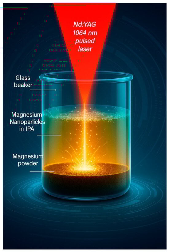
Figure 1.
Schematic of the pulsed laser ablation in liquid process (PLAL) showing Mg powder ablation in isopropanol alcohol.
Despite the relatively low cost of PLAL and over two decades of active research with hundreds of published studies, the field remains underutilized in industry [7,8]. The key barriers are the complexity of input–output relationships and the low concentrations of the resulting colloids. However, machine learning (ML) has the potential to transform this landscape by predicting NP properties directly from laser processing parameters, thereby accelerating optimization and reducing the need for extensive experimental campaigns. To date, few studies have applied ML specifically to PLAL, representing a significant gap in the literature that this work aims to address [7,8]. While some notable efforts have applied ML to laser processing more broadly, specific use cases involving NP synthesis via PLAL remain limited.
Tsai et al. [9] applied ML to optimize laser ablation parameters in the CMOS-MEMS process, focusing on silicon nitride films. Their study used supervised classifiers including Extreme Gradient Boosting (XGBoost), Random Forest (RF), and Logistic Regression (LR) to categorize ablation quality based on laser fluence and laser processing time (similar to ablation time in PLAL). Key findings revealed the existence of a fluence threshold above which further increases in laser processing time did not significantly improve ablation quality. XGBoost outperformed the other models with classification accuracies up to 0.78, demonstrating its effectiveness for identifying complex relationships in laser processing datasets. Although the application focused on post-CMOS Si3N4 removal rather than NP synthesis, the use of data-driven methods to link laser processing input parameters with process outcomes aligns closely with the goals of PLAL process optimization. Importantly, this study reinforces the value of XGBoost in high-dimensional laser processing datasets and highlights the potential of ML for parameter prediction and quality assurance.
Yildiz [10] demonstrated the potential of artificial neural networks (ANNs) in accurately predicting laser ablation efficiency during neurosurgical applications using a 1940 nm thulium fiber laser. The study utilized 12 experimental and four validation data points of laser ablation on cortical and subcortical ovine brain tissue (a total of 16 data points). Inputs included laser mode, laser fluence or power, laser processing time (analogous to ablation time in PLAL), and thermal metrics, while the ANN output was the ratio of ablated to thermally altered area. The optimized ANN achieved ablation efficiency prediction mean absolute error (MAE) as low as 2.1% and classification accuracy of 88% for optimal laser mode selection (continuous vs. pulsed). Notably, the study confirmed the capability of ANNs to model complex, nonlinear relationships between multiple laser parameters and thermal effects, especially under small data conditions. While this work focused on thermal damage in soft tissues for medical laser ablation, its core findings align with challenges in PLAL-based NP synthesis—namely, the need to manage multidimensional, nonlinear input–output mappings under sparse data regimes. Yildiz’s work exemplifies how ML can improve precision and parameter optimization in laser-material interactions, supporting the approach to applying ML-based models to PLAL for predictive control over NP size and concentration.
Wang et al. [11] also demonstrated the impact of ML in predicting outputs using laser processing parameters as features during femtosecond laser-induced periodic surface structures (LIPSS) studies. Their study used several ML models for predictions, including ANN, RF, decision tree (DT), support vector machine (SVM), k-nearest neighbors (KNN) and Naive Bayesian Classifier algorithms, for the prediction of laser processing outputs. The results show that DT gives the best accuracy of 97% and provided fast processing and good explainability of how the classification was performed, another advantage of DTs over the other algorithms. In their study, k-fold cross-validation with k = 5 was used to prevent the data overfitting problem, especially for a small dataset. Their data collection process involved laser processing of Ti6Al4V surfaces at various laser processing parameters. The parameters were generated by a uniform sampling method (laser power varied from 1 to 5 mW, scanning speed from 0.5 to 1.5 mm/s and scanning number from 1 to 5 times), resulting in a dataset of 150 samples. For feature characterization, scanning electron microscope (SEM) was used to examine the LIPSS and images were collected, labelled by human inspection (and k-means clustering), and stored for machine learning processing.
Oh and Ki [12] presented a groundbreaking data-driven deep learning model for predicting hardness distributions in the laser heat treatment of steel (a laser processing method similar that reassembles PLAL). They used a Conditional Generative Adversarial Networks (cGANs)-based Convolutional Neural Network (CNN) encoder–decoder to map a single cross-sectional temperature snapshot—captured at peak surface temperature following a 3D thermal simulation—to corresponding hardness profiles. Trained on only three laser processing conditions that were augmented to 213 samples via sliding-window cropping, the network delivered an impressive 94% accuracy, significantly outperforming a physics-based carbon diffusion model (85%). Their study addressed a key issue that can hinder ML in PLAL research, which is the limited data (small datasets) due to the time and resource consuming nature of experiments. With just three experiments, they were able to add synthetic data to increase the data size to 213 rows and produced a highly accurate model. Data augmentation should, therefore, be considered when training ML models suing PLAL data to potentially reduce model errors. Other studies have also shown the positive impact of data augmentation during training ML models, including KNN [13] and DTs [14] models.
Park et al. [15] highlighted in their perspective review paper, the need to automate NP synthesis to overcome the limitations of traditional trial-and-error methods, which are slow, manual, and inefficient for exploring large experimental parameter spaces. Producing consistent and functional NPs requires fine control over synthesis conditions, which is something difficult to achieve without automation due to the complexity and nonlinearity of the process. They added that integrating robotics, real-time characterization, and machine learning allows for the development of closed-loop systems that can intelligently plan, execute, and optimize experiments. This approach speeds up the discovery and tuning of NP properties while minimizing human effort and experimental cost. The research team added that, although full automation across all steps is still a work in progress, advances in robotic platforms and ML models are rapidly closing the gap. Automating synthesis workflows is especially important for scaling from lab to pilot production, where conditions often differ significantly. The use of automated systems ensures greater reproducibility, faster optimization, and better scalability, making NP synthesis technologies, such as PLAL, more accessible for real-world applications.
Bakhtiyari et al. [16] also agreed with Park et al. [15] in their recent review article that advancing NP synthesis requires shifting from manual, trial-based experimentation to automated, intelligent recommender systems that can recommend processing parameters. Traditional synthesis approaches struggle with navigating the vast and complex parameter space needed to reliably produce NP with precise size and concentration. In their review paper, they concluded that these manual methods are time-consuming, lack reproducibility, and are unsuitable for industrial scaling. The integration of robotic synthesis platforms, automated characterization tools, and machine learning models offers a solution. Bakhtiyari et al. [16] added that closed-loop frameworks—where machines learn from each experiment and iteratively refine the process—enable the rapid exploration of synthesis conditions while minimizing human intervention, whereby ML, can recommend optimal experiments, reducing time and cost. The article emphasizes that while full automation is not yet universally achieved, progress in each stage—from synthesis to property evaluation and structural analysis—is rapidly accelerating. Automation is also critical for scaling up from laboratory to production, where variables, such as heat and mass transfer, differ significantly. They finished by stating that, ultimately, automating NP synthesis is not just a matter of efficiency; it is essential for consistent, scalable, and intelligent materials discovery.
Prediction of outputs based on laser processing parameters alone is insufficient for real-world industrial and practical applications. The integration of recommender systems enables the construction of intelligent databases that can guide users or robots in selecting appropriate processing parameters to achieve desired NP size and concentration combinations. Recommender systems assist users in making informed decisions. Common applications include shopping platforms, such as Amazon, where items are recommended based on previously selected products (content-based recommenders), or music streaming services like YouTube or Spotify, where popular content is suggested based on collective viewing trends (ranking-based recommenders). In research, recommender systems are increasingly being explored for tasks, such as material selection, and, in this case, processing parameter optimization. This approach allows users—regardless of their familiarity with PLAL—to operate laser systems efficiently by inputting the desired NP characteristics and following system-generated recommendations. Such advancements can significantly reduce the need for iterative experiments and complex characterization, potentially accelerating the industrial adoption of PLAL by bringing the technology to a higher technology readiness level (TRL). Herein, seven machine learning models, including Decision Trees (DT), Random Forest (RF), Extreme Gradient Boosting (XGBoost), Support Vector Regression (SVR), k-Nearest Neighbors (KNN), Multiple Linear Regression (MLR), and Multiple Polynomial Regression (MPR), are explored in predicting magnesium NP size and concentration during PLAL of magnesium powder. After NP size and concentration prediction, the best ML model is used to produce a database from which a recommender system is developed to recommend laser processing parameters (ablation time, laser fluence, and laser scan speed) based on the required combination of NP size and concentration. The ML models are selected based on a combination of five evaluation metrics during the regression task, including root mean squared error (RMSE), mean absolute percentage error (MAPE), mean percentage error (MPE), mean absolute error (MAE), and R-squared value (R2). Two recommender systems, based on either Cosine similarity or KNN, are compared and the best is picked for deployment. This work addresses a key literature gap whereby we move PLAL from an experimental trial-and-error phase to a more practical phase where processing parameters are recommended by ML, which goes towards fully or semi-automated nanoparticle production systems.
2. Materials and Methods
2.1. Data Collection (Pulsed Laser Ablation in Liquid Experiments)
A 3 × 3 full factorial design of experiments (DOE) with 3 replicates was used to produce the dataset after preliminary experiments. To produce the Mg NPs, magnesium powder (99% purity, 0.06–0.3 mm diameter, Sigma Aldrich Ireland Limited, Wicklow, Ireland) was ablated at different laser processing parameters. A Nd:YAG laser system (WEDGE HF 1064, Bright Solutions, Cura Carpignano, Italy) with pulses centered at 1064 nm was used for ablation experiments in a batch mode set-up. A schematic of the PLAL process is shown in Figure 1 where we can see the powder on the bottom of the beaker, the isopropyl alcohol (IPA) liquid on top, and the Mg NPs within the IPA liquid following laser ablation. IPA was used as a liquid medium as it was found to be more compatible with Mg particles than water (water reacts with Mg powder). There was no mixing or reaction between the powder and IPA (one of the reasons why IPA was selected as a liquid medium), the powder particles simply sink at the bottom of the IPA due to its higher density. The repetition rate was kept constant at 10 kHz and the pulse width was kept at 0.6 ns. Three ablation times (2, 5, and 25 min), three laser fluences (1.83, 1.88, and 1.91 J/cm2) and three laser scan speeds (3000, 3250, and 3500 mm/s) were considered. Three samples were produced at each set of the 27 sets of process parameters, resulting in a dataset of 81 datapoints based on a combination of these three features (ablation time, fluence, and laser scan speed). After NP synthesis each sample was characterized to produce the two target variables which are mean nanoparticle diameter (nanoparticle size) and nanoparticle concentration.
The nanoparticle size was measured via Dynamic light scattering (DLS). Zetasizer Nano ZS system (Malvern Instruments Ltd., Worcestershire, UK). DLS system was used for NP size measurement and 10 DLS runs/measurements (2 min each) were conducted for each sample and averaged automatically by the software. The DLS give a direct NP mean size for each measurement (mean particle diameter size) and these were recorded for each experiment, taking an average of 10 repeated recordings for each experiment. The NP concentration and plasmonic peak outputs were measured via Ultraviolet Visible spectroscopy (UV–Vis). UV–Vis spectroscopy was conducted with a Varian Cary 50 UV–Vis spectrophotometer using a quartz cuvette (10 mm path length, Helma). The scan range was 190–900 nm with a scan rate of 600 nm/min. The absorbance value at the signature peak (204 nm) was used as a measure of NP concentration in accordance to Beer Ambert’s Law as shown in Equations (1a) and (1b). For each NP concentration measurement, 1 μL of the colloid was diluted into 1 mL of IPA (a dilution factor of 1000) to avoid spectra saturation. The concentration was calibrated (factoring in the 1000 dilution factor) and an absorbance record of 1 in the diluted sample represented a concentration of 2 mg/mL; however, for simplicity, the raw UV–Vis recordings (unitless) are used as a measure of concentration, which can easily be translated to mg/mL by multiplying each value by 2. Field emission scanning electron microscopy and scanning transmission microscopy (STEM, Hitachi S5500 Field Emission SEM instrument) was used to study the NP morphology and size as a qualitative measure but not used in generating the dataset for training ML models (SEM was used just for NP visualization). One μL of colloid was pipetted onto a copper SEM grid for analysis; no drying time was needed as IPA evaporates quickly. A thin powder layer (2 mm thickness) was carefully placed and evenly spread on the bottom of a glass beaker (60 mm diameter). A 3 mm height of liquid (IPA) above the powder layer was ensured for each sample. Fresh powder was used for each PLAL data collection experiment. The laser scanning pattern was in a spiral shape (outer diameter of 55 mm) with a hatch spacing of 50 μm. Each PLAL experiment was carefully timed using a stopwatch and the resulting nanocolloid was immediately collected by carefully pipetting some of the colloid (5 mL) on top of the remaining powder using a standard plastic pipette, ensuring that no powder particles (large particles) were collected. The as-collected magnesium colloid of ink was used in characterization processes without any filtration process to avoid this post processing to bias the results.
where,
- A = Absorbance (unitless)
- ε= Molar absorptivity (or molar extinction coefficient) in L/mol·cm
- C = Concentration of the absorbing species in mol/L
- L = Path length of the sample cell in cm (10 mm in this case)
- Absorbance (A) is related to the intensity of incident (I0) and transmitted (I) light by
2.2. Machine Learning Algorithms and Hyperparameter Tuning
The dataset was randomly split into a testing and training set with a 20:80 split, respectively. Seven ML models were trained in regression mode on the training dataset including Decision Trees (DT), Random Forest (RF), Extreme Gradient Boosting (XGBoost), Support Vector Regression (SVR), k-Nearest Neighbors (KNN), Multiple Linear Regression (MLR), and Multiple Polynomial Regression (MPR). One model was selected for further development and deployment based on predictive performance and computational efficiency. Model evaluation was performed using five regression metrics, namely R-squared (R2), Mean Absolute Error (MAE), Mean Percentage Error (MPE), Mean Absolute Percentage Error (MAPE), and Root Mean Squared Error (RMSE). Each model was used to predict NP mean size and NP concentration independently, and the results were compared to identify the optimal model for each output variable. The best model among these was employed to generate synthetic datasets (augmented datasets) by predicting NP characteristics for a wide range of processing parameters. These augmented datasets serve as the foundation for constructing a database for a recommendation system. Cosine similarity and the KNN algorithms were utilized in building recommender systems that can recommend laser processing parameters based on user-defined targets for NP mean size and concentration. The recommender system returns either an exact match or the closest available configuration from the database (formed using the predictions from the ML models). All model training and recommender system implementation were conducted using Python version 3.12.7. A schematic overview of the methodological framework is presented in Figure 2. The remainder of this section outlines the rationale for selecting the seven regression models and the two recommendation algorithms, including details of the hyperparameter tuning procedures.
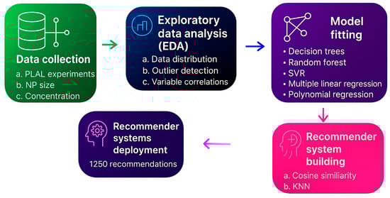
Figure 2.
Schematic of the sequential steps in this study starting at experimental steps (data collection), through the data analytics procedure, model fitting and comparison, recommender system building, and ending at recommender system deployment.
2.2.1. Decision Trees
DT can work both in classification mode and regression mode. In regression mode, DTs partition data based on error measurements, such as mean absolute error or room mean squared error; the user needs to define the matric used. Similarly, in classification mode, DT partitions data based on information gain, which is calculated using either entropy (Hs) or Gini impurity (Hs), as shown in the schematic in Figure 3a. At each node, the DT algorithm computes the information gain (IG) for each feature and selects the feature with the highest IG to split the data. This process is repeated recursively until the data is fully partitioned into leaf nodes (also called termination node), where no further splitting is possible. Entropy, Gini impurity, and information gain are given by Equations (2)–(4), respectively, where H(s) represents entropy or Gini impurity, Pi is the proportion of samples in a given class/category, C is the number of classes, |Sv| is the number of examples in S for which feature A takes value V, |S| is the total number of examples in S, and H(Sv) is the entropy of the subset Sv. The hyperparameters tuned in the decision tree regressor are presented in Table 1, including before tree construction pruning strategies, such as restricting the maximum depth of the tree to 3, 4, 5, and 10 layers. An option of no depth restriction (no pruning) is also explored as shown in Table 1.
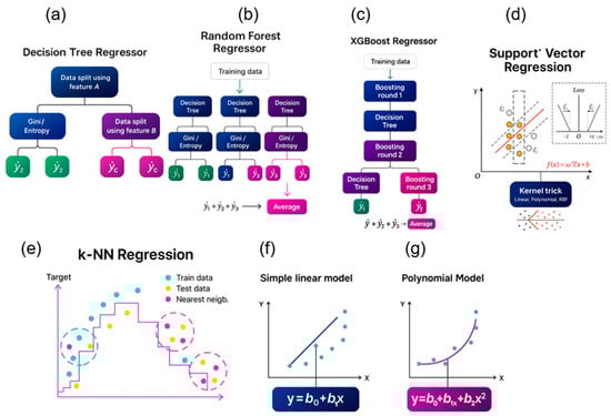
Figure 3.
Schematic representation of (a) a decision tree regressor, data is split at each node using the feature with the highest information gain calculated by Equation (3); (b) Random Forest regressor, which uses multiple decision trees gives a mean result from the outputs of the decision trees; (c) support vector regressor; (d) k-nearest neighbor; (e) multiple linear regression; (f) multiple polynomial regression, and; (g) polynomial regression.

Table 1.
Hyperparameter tuning using grid search k = 5 cross-validation.
2.2.2. Random Forest
Random Forest is an ensemble model, meaning it is not a standalone algorithm but rather, is composed of multiple instances of another model, in this case, decision trees. RF is designed to improve upon DT algorithm by aggregating the predictions of multiple trees, thereby reducing error, as illustrated in the schematic in Figure 3b. However, RF does not always outperform a single DT; in some cases, a simpler model yields better performance; such a case was reported by Wang et al. [11], who reported the DT algorithm attaining higher classification accuracy than random forest (and other models). If the errors from individual trees propagate into the ensemble, RF may even produce higher overall error than a well-tuned single DT. That said, with appropriate hyperparameter tuning, RF can outperform a single DT by mitigating overfitting and achieving better generalization. Tree-based models are particularly effective for numerical data in both regression and classification tasks. They are computationally efficient and offer interpretability, making them highly suitable for use in AI workflows. For these reasons, DT, RF, and XGBoost—each a tree-based model—were selected for the regression task in this study, as they are expected to achieve low prediction errors. In addition, the existing literature supports the application of these models to numerical datasets, reinforcing their inclusion in this work. The hyperparameters tuned for the RF model are presented in Table 1. These include number of DTs (2, 5, 10, or 20) and tree pruning strategies before tree construction.
2.2.3. XGBoost
XGBoost, like Random Forest, is an ensemble model composed of multiple DTs. The key distinction is that rather than averaging outputs as RF does, XGBoost builds trees sequentially. Each new tree is trained to correct the errors made by the previous one, as illustrated in the schematic in Figure 3c. This iterative approach is intended to enhance performance over both RF and individual DTs. Nevertheless, XGBoost does not consistently outperform a single DT. For this reason, DT, RF, and XGBoost are all evaluated in this work. One contributing factor to XGBoost’s potential underperformance over simple DTs is its tendency to overfit, particularly on small or noisy datasets. In such instances, the simplicity of a single DT can lead to better generalization, while the complexity of XGBoost may result in fitting to noise rather than underlying patterns. Additionally, XGBoost demands extensive hyperparameter tuning; without proper optimization, its predictive performance may be inferior to that of a well-tuned DT. Furthermore, ensemble models, such as RF and XGBoost, require significantly more computational resources and processing time than simpler models like DT. Thus, final model selection should balance prediction accuracy with computational efficiency. The hyperparameters tuned for the XGBoost model are presented in Table 1.
2.2.4. Support Vector Regression
Support Vector Regressor (SVR), also known as Support Vector Machine (SVM) when used for classification, is a powerful and well-established model that performs effectively on numerical data, making it a suitable choice for this study. SVR operates based on the kernel trick [17,18], a technique in which data is projected from a lower-dimensional space into a higher-dimensional feature space to enable separation that may not be possible in the original space. This is illustrated in Figure 3d. The kernel function defines the hyperplane that separates the data in the transformed space, allowing the model to handle both linear and nonlinear relationships. SVR requires feature engineering which involves standardizing the data or scaling the data.
Several kernel functions are available for SVR, and the four most common ones are explored in this work:
- Linear kernel, which is effective when the relationship between features and target is approximately linear;
- Polynomial kernel, suitable for modeling more complex relationships with curved boundaries;
- Radial Basis Function (RBF) kernel, widely used for its ability to capture highly nonlinear patterns;
- Sigmoid kernel, which also models nonlinear relationships but behaves differently due to its resemblance to activation functions in neural networks.
Each kernel brings unique advantages depending on the nature of the data. Their inclusion ensures that the SVR model is flexible enough to capture a wide range of trends present in the dataset. The hyperparameters tunned in the SVR are presented in Table 1.
2.2.5. K-Nearest Neighbor
KNN is a distance-based model and operates differently from the previously discussed models, offering a unique prediction mechanism that may outperform others depending on the dataset. KNN is well-suited for numerical data and, similar to SVR, requires feature standardization. This is because the algorithm relies on distance calculations, and features with larger values can disproportionately influence predictions if the data are not standardized. The working principle of KNN is illustrated in Figure 3e, where new data points are compared to their nearest neighbors from the training set to make predictions. Equations (4) and (5) present the mathematical formulation underlying the KNN algorithm. In Equation (5), the output or prediction ((x)) based on the input point x, (Yi) is the output value (target) of the ith neighbor, k is the number of nearest neighbors considered, and Nk(x) is the set of indices of the k nearest neighbors of x. The nearest neighbors are calculated based on the distance and this can be calculated in a number of different ways; however, Euclidean distance is the most used method, represented by Equation (6), whereby n is the number of features, xj and xij are the jth feature values of the test point and the ith training point, respectively. The hyperparameters tunned in the KNN are presented in Table 1, including how the distance between neighbors is calculated, which is controlled by hyperparametric ‘p’. Setting p = 1 uses Manhattan distance, which calculates distance based on the sum of absolute differences while setting p = 2 uses Euclidean distance, which calculates distance-based straight-line distance.
2.2.6. Multiple Linear Regression
Multiple linear regression (MLR) is among the simplest AI models—so common that it is sometimes overlooked as part of the AI landscape. It fits data to a linear equation and is, therefore, most effective when the underlying patterns are linear. Given the nonlinear nature of PLAL, MLR is not expected to perform strongly, particularly for NP size prediction. Nonetheless, it was selected for its simplicity and to serve as a baseline for comparison with more complex models, such as DT and KNN. Equations (7)–(9) shows the working mechanism of MLR (Ordinary least squares) whereby Y is the predicted value (output), b0 is a constant, bi is the weighting of input feature i, and Xi is ith input feature. and represent the mean of the ith feature in the training dataset and the mean of the output in the training dataset, respectively, and k represents the kth row or kth datapoint of the training dataset. There are not many hyperparameters to tune in MLR as shown in Table 1, making it a fast model to fit, another advantage over the AI models and its mechanism is shown in the schematic in Figure 3f.
2.2.7. Multiple Polynomial Regression
The hyperparameters tuned for the MPR model are presented in Table 1. Similar to MLR, there are relatively few hyperparameters to optimize, which makes MPR a fast model to train—an additional advantage over more complex AI models. Its underlying mechanism is illustrated in the schematic in Figure 3g. MPR may offer improved performance over MLR as it is capable of capturing certain nonlinear relationships inherent in PLAL. The model allows for the inclusion of polynomial terms of varying degrees (in this case squared and cubic terms were considered), adding complexity and flexibility compared to MLR. Despite this added complexity, both MLR and MPR can be summarized using a single equation, making them the most interpretable models among the seven evaluated in this study.
2.2.8. Evaluation Metrics
Five evaluation metrics were used to evaluate the models discussed in the previous sections to ensure that the models are evaluated from different perspectives. The evaluation metrics considered for each model are the following:
- 1.
- R-squared value (R2):
R2 quantifies how much of the variability in the dependent variable is explained by the model. It is an effective metric for understanding how well the model fits the data and is useful when comparing models trained on the same dataset. R2 is highly affected by extreme values, which can skew the score and lead to misleading interpretations of model performance. While R2 indicates the proportion of variance explained, it does not communicate the actual size of the errors in practical terms. Thus, it lacks direct interpretability regarding prediction accuracy.
- 2.
- Mean absolute error (MAE):
MAE calculates the average of the absolute differences between predicted and actual values. Because it uses absolute values rather than squared differences, it gives a straightforward, unit-consistent measure of prediction error. Unlike RMSE, which squares errors and exaggerates the influence of outliers, MAE treats all errors equally. Because of its simplicity and interpretability, MAE is widely used across various domains—especially where equal importance is placed on all errors. While this may be an advantage in some cases, it can be a disadvantage in contexts where large errors are particularly costly. MAE treats a 1-unit error and a 10-unit error linearly, with no additional penalty. This makes it more robust in datasets with occasional large deviations. However, because it uses absolute values, the negative and positive errors can cancel out leading to unrealistically low mean error values. Since MAE does not square the errors, it provides less insight into the variance or distribution of errors, which may limit its usefulness for comparing highly variable datasets.
- 3.
- Mean percentage error (MPE):
MPE calculates the average percentage difference between predicted and actual values. This makes it useful when you want to interpret errors relative to the magnitude of actual values, such as in financial forecasting or sales data. Unlike MAPE, MPE retains the sign of the errors. This allows it to reflect whether a model systematically overpredicts (positive MPE) or underpredicts (negative MPE), making it a useful diagnostic for model bias. If actual values are close to zero, MPE can become extremely large or undefined, leading to misleading or unusable results. Since MPE preserves the sign of errors, positive and negative deviations can offset one another. This can result in a deceptively low MPE just like MAE, even if individual prediction errors are large. MPE can misrepresent performance in datasets with wide-ranging values or asymmetrical distributions, as it focuses on relative rather than absolute error.
- 4.
- Mean absolute percentage error (MAPE):
MAPE presents errors in percentage terms, which makes it intuitive and easy to interpret for nontechnical stakeholders. This makes it ideal for communicating performance to broader audiences. Unlike RMSE, MAPE remains relatively stable even in the presence of a few extreme values. It does not exaggerate the impact of outliers, particularly when the actual values are also high. Conversely, when actual values are close to zero, MAPE can become misleading by inflating error percentages drastically, which could distort the accuracy interpretation. Additionally, MAPE might significantly understate the severity of prediction errors when actual values are large, leading to a falsely optimistic impression of model performance.
- 5.
- Root mean squared error (RMSE):
RMSE calculates the square root of the average squared differences between predicted and actual values. This provides a clear measure of the magnitude of prediction errors and emphasizes larger errors, making it valuable when precision is critical. It is a good measure when large deviations are priority. RMSE is particularly suitable for applications where large prediction errors are especially costly or undesirable. It penalizes larger deviations more heavily than other metrics like MAE or MAPE. On the other hand, because errors are squared before being averaged, RMSE can be disproportionately influenced by outliers, potentially misrepresenting the model’s typical performance if large errors are infrequent but extreme. Furthermore, unlike MAPE, RMSE does not offer a percentage-based view of the error, which can make it harder for stakeholders to interpret the results in a relative context.
GridsearchCV was used during hyperparameter tuning to select the best hyperparameters for both NP size and concentration predictions. The hyperparameters achieving the highest R2 value in k = 5 cross-validation during training were selected. R2 was selected because models were doing much better in other evaluation metrics than in R2; therefore, to ensure that the models captured maximum variability in the data, R2 was used. Final model selection was then based on the evaluation of all five metrics described earlier.
2.3. Recommender Systems
After selecting the best-performing models from the seven presented in Section 2.2—based on a balanced assessment across the five-evaluation metrics discussed in Section 2.2.8—two recommender systems were developed and compared. The better of the two was selected for deployment and further analysis. The recommender systems are designed to suggest laser processing parameters (ablation time, laser scan speed, and laser fluence) that yield the desired NP size-concentration combination (instead of individual predictions). To achieve this, the system searches a database for the most similar set of processing parameters expected to produce an output closest to the requested combination of NP properties. The database used by the recommender system is generated using the predictive ML models. The best models for NP size and NP concentration prediction were used to generate synthetic outputs for various random combinations of laser processing parameters sampled from the original 3 × 3 full factorial DOE. Two versions of the database were constructed: a smaller set containing 331 entries (81 experimental data points plus 250 predictions) and a larger set with 1331 entries (81 experimental data points plus 1250 predictions). This dual-database approach was employed to examine the effect of database size on recommendation accuracy. Recommendation accuracy was evaluated using MAPE, calculated between the requested output values (NP size and concentration) and the values corresponding to the recommended parameter set.
One of the recommender systems is based on Cosine Similarity, which calculates the angle between two vectors and uses the value as a measure of similarity. The vector (or row) with highest similarity to the user-requested outputs is recommended. Equation (10) shows the basis of Cosine Similarity where w1 and w2 are two n-dimensional vectors (rows in a dataset in this case), each represents an entity (a feature set in this case), w1j and w2j are the j-th components (or entries or columns in this case) of vectors w1 and w2, respectively. The numerator calculates the dot product of vectors w1 and w2, measuring the similarity in the direction between the two vectors. The summation runs over all n components of the vectors. Cos (θ) is between 0 and 1 with a value closer to 1 showing similarity between the two rows, or entries under comparison.
The second recommender system is based on KNN, which calculates the distance between vectors using Euclidean distance, as shown in Equations (5) and (6). The database entry with the smallest distance to the requested outputs (NP size-concentration combination) is returned as the recommended set of processing parameters. The accuracy of this recommendation is assessed using MAPE, which quantifies the similarity between the requested and predicted outputs, and is used to compare the two systems. To evaluate recommendation performance, 100 random combinations of NP size and concentration were generated using Excel’s random number generator. These values were constrained within the minimum and maximum observed values of NP size and concentration in the database. The same set of 100 randomly generated outputs was used to test both recommender systems. The system that yielded the lower MAPE across all test cases was selected for further analysis and recommended for real-world deployment.
3. Results and Discussion
3.1. Exploratory Data Analysis (EDA)
The as-fabricated Mg NP colloids or inks are shown in the photograph in Figure 4, where the color intensity of each colloid is influenced by both NP size and concentration. Inks produced with a 2-min ablation time generally appear grey, while longer ablation durations result in a pale yellow to dark yellow/brown color. This variation arises because different NP sizes absorb light at different wavelengths, and the intensity of this absorption depends on the number of absorbing species (NP concentration). The observed color differences suggest that ablation time influences both NP size and concentration. This hypothesis is examined further through data analysis later in this section.
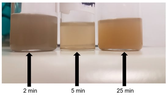
Figure 4.
Images of magnesium nanoparticle colloids produced at various ablation times including 2 min (left), 5 min (middle), and 25 min (right).
The NPs were predominantly spherical, as expected, as shown in Figure 5. Figure 5a–c illustrate that some samples contain very small particles, approximately 20 nm in size. However, due to the measurement method used, the mean diameter is skewed by the presence of larger particles. In such cases, where a high proportion of small NPs is present, the Mean Number Diameter method is most appropriate. Other size measurement methods will be discussed in Section 4. Particle aggregation is evident in Figure 5a,b, where NPs appear attached to each other in tree-like networks. This is likely due to covalent bonding and Van der Waals forces, which may cause NP size measurements to reflect larger sizes than the actual individual particles. Nevertheless, if this effect is consistent across all samples, the DLS measurements remain reliable for comparative purposes, though the true NP sizes may be smaller in the absence of aggregation. Figure 5d shows the UV–Vis spectra of the as-fabricated Mg inks, all of which display a distinct absorbance peak at 204 nm. The magnitude of this peak corresponds to NP concentration, consistent with Beer–Lambert law (Equation (1)). Absorbance values were recorded for each of the 81 samples, forming the dataset used for NP concentration prediction (Section 3.2), and ultimately for developing the recommender system (Section 3.3), which recommends PLAL parameters required to produce a specified NP concentration and size.
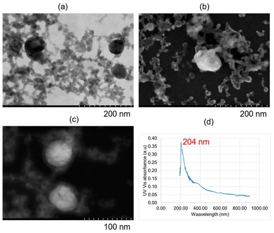
Figure 5.
Electron microscopy images of magnesium nanoparticles (a) using bright field-transmission electron microscope at an excitation voltage of 30 kV; (b) using scanning electron microscopy at an excitation voltage of 5 kV; (c) using dark field-transmission electron microscope at an excitation voltage of 30 kV; and (d) ultraviolet–visible spectroscopy of magnesium nanoparticles.
The correlation heat map in Figure 6 was used to analyze correlations between the variables. All the input parameters had zero correlation with each other giving them similar importance at this stage in terms of predictions. The ablation time has a strong positive correlation with the NP concentration (0.94), this a longer ablation time produces more NPs as expected. Longer ablation times tend to produce smaller NP sizes also as expected. With longer times, the secondary ablation process begins to occur whereby the primary NPs can still absorb laser photons, leading to fragmentation. This is not always the case in ablation processes as sometimes longer ablation times can lead to larger particles via the process of melting and reforming of larger NPs due to the newly available Gibbs free energy from secondary laser photon absorptions. Primary nanoparticles can also get sucked into an ablation plume and cavitation bubble events leading to particle attachment or reforming which can result in larger particles. But usually, smaller particles are formed. The NP concentration is also slightly negatively correlated to the NP size. As more NPs are added to the mix, the mean size tends to become smaller, which is attributed to secondary laser absorptions, a term called laser fragmentation in liquid (LFL).
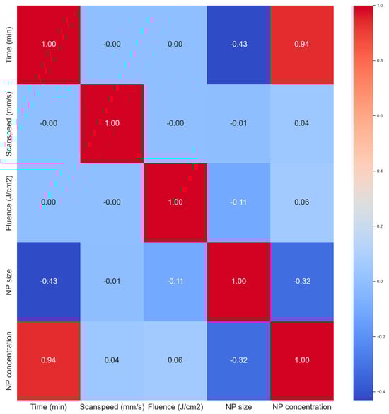
Figure 6.
Correlation matrix (heat map) of the dataset.
The histogram of the NP size is shown in Figure 7a. The distribution looks close to normally distributed with the mean size just above 100 nm. The NP concentration distribution is bimodal as shown in Figure 7b with concentrations on the small sizes. These usually need to be avoided for most applications since most applications require a high BNP concentration. The box plots show that the NP size distribution is almost even with no outliers while the NP concentration is skewed to the right and also without any outliers. Outliers tend to cause difficulties in machine learning models, and their absence here makes the prediction problem easier. Also, a lack of outliers shows some level of consistency in the data collection process (experiments and characterization).

Figure 7.
Histogram showing the distribution of nanoparticle (a) mean diameters and (b) concentration. Box plot showing the distribution of nanoparticle (c) mean diameters and (d) concentration.
The violin plot (Figure 8a) of the NP size data shows that the distribution is roughly symmetric with a slightly wider spread between 100 and 175 nm. The data suggests most NPs tend to fall in the 125–150 nm size range, indicating a consistent synthesis process. There is a high density of values centered around 125–150 nm (thickest part of the violin) and the white dot (median) is well-centered, showing a balanced distribution without significant skew. As for the NP concentration violine (Figure 8b), the distribution is skewed to the right (positively skewed), most values are concentrated around 0.5, but there is a long tail toward higher concentrations (~2.5), the white median dot lies close to the bottom, supporting this skew. The shape indicates bimodality or clustering, especially noticeable bulges around 0.5 and 2.0. The data suggests that are two major different conditions or regimes in your synthesis that are yielding different concentration levels, and ablation time seems to be the most contributing factor to the concentration according to the correlation heat map in Figure 6. The bimodal distribution is primarily caused by the difference between short (2 and 5 min) and long (25 min) ablation times. The skew in the data indicates that most experiments resulted in lower concentrations, with only a few producing higher absorbance values. This trend aligns with the design of experiments (DOE), where 66.7% of the runs were performed at shorter ablation times (2 and 5 min).
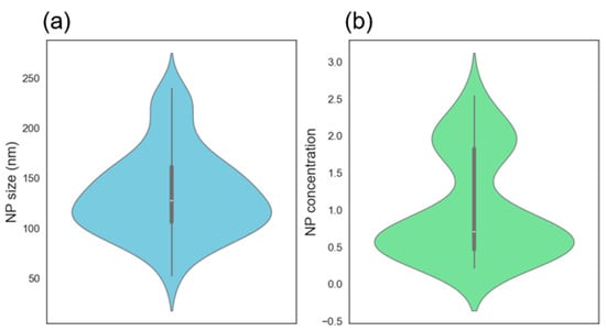
Figure 8.
Violin plot showing the distribution of nanoparticle (a) mean diameters and (b) concentration.
Furthermore, summary statistics were used to establish a data-driven threshold for acceptable model error. Specifically, the standard deviation or standard error was calculated for each of the 27 experiments in the 3 × 3 DOE. Each experiment was repeated three times, resulting in a dataset of 81 samples. The variation among these three replicates was quantified using standard deviation or standard error, which defines the permissible error range that the ML models can aim to match or exceed. The standard deviations for each experiment, covering both NP size and concentration, are presented in Table 2. These values were then averaged to obtain an overall estimate of experimental variability. As shown in Table 2, average MAE or RMSE values of 27.2 nm for NP size and 0.15 for concentration represent the baseline error limits, corresponding to the average experimental standard deviations. These values are considered optimal targets for ML model performance, as the models cannot be expected to predict with greater accuracy than the inherent experimental variability. This performance ceiling can be lowered by increasing the number of experimental replicates. While three repeats are standard practice in scientific research and provide a realistic representation of experimental conditions, additional repetitions are known to reduce experimental error. It is important to note that this baseline standard error constitutes the maximum achievable accuracy for the AI models, beyond which further improvement is not feasible without reducing experimental uncertainty.
Table 2.
Summary statistics for each or the 27 experiments.
3.2. Machine Learning Models
The optimal hyperparameters for each model, identified using GridSearchCV with five-fold cross-validation and based on the highest R2 values, are presented in Table 3. The traditional regression models exhibited the highest errors across all metrics and showed significant overfitting, indicated by large discrepancies between training and testing results. Although these models offer the advantage of faster training and inference times, they failed to capture the nonlinear relationships present in the concentration prediction task. While polynomial regression can model certain nonlinear effects, the minimal performance difference compared to the simple MLR model suggests limited nonlinear structure in the data. This is evident from the similar results observed in both the concentration predictions (Figure 9) and NP size predictions (Figure 10). Despite these limitations, all models achieved high R2 values of at least 89%, indicating that the majority of data variability was captured. The KNN model achieved the highest R2 value, as reported in Table 4. Overall, model performance across evaluation metrics was strong, with RF and XGBoost demonstrating particularly good generalization, evidenced by lower testing errors. The prediction errors appeared balanced, with both overestimations and underestimations distributed evenly, as shown by the mean percentage errors in Figure 9d, which remained within ±10%. The predictive accuracy of XGBoost was notable, with MAE and RMSE values of 0.12 and 0.15, respectively. These values fall below or equal to the experimental standard deviation of 0.15 determined during EDA in Section 3.1, making them acceptable within the bounds of experimental uncertainty. Therefore, an absolute error below 0.15 is considered satisfactory given the inherent error in the raw data.
Table 3.
Optimized hyperparameters for each machine learning model with k-fold cross-validation (k = 5) found via GridSearchCV.
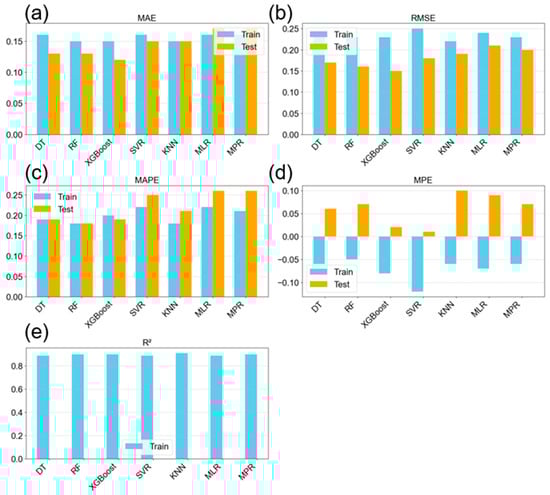
Figure 9.
Evaluation metrics of the seven models from k = 5 cross-validation, showing both training and testing results for the prediction of the nanoparticle concentration; (a) mean absolute error; (b) root mean squared error; (c) mean absolute percentage error; (d) mean percentage error; and (e) R-squared value.
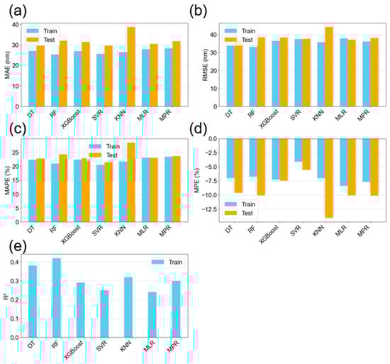
Figure 10.
Evaluation metrics of the seven models from k = 5 cross-validation showing both training and testing results for the prediction of the nanoparticle mean diameter; (a) mean absolute error; (b) root mean squared error; (c) mean absolute percentage error; (d) mean percentage error; and (e) R-squared value.
Table 4.
Evaluation metrics of the seven models from k = 5 cross-validation, showing both training and testing results for the prediction of the nanoparticle concentration.
Model predictions for NP mean diameter are summarized in Table 5 and visualized in Figure 10. In this case, the R2 values were generally lower than for concentration, indicating greater difficulty in modeling NP size. This aligns with the EDA findings, which showed stronger feature correlations and lower variability for concentration than for NP mean diameter. The RF model achieved the highest R2 for NP size prediction (Figure 10e) and ranked among the top performers across all evaluation metrics. Interestingly, despite having a slightly lower R2, the DT model outperformed RF in terms of absolute error, achieving MAE, RMSE, and MAPE values of 30 nm, 37 nm, and 23%, respectively. These errors are comparable to the experimental standard deviation of 27 nm, suggesting that the model delivers predictions within an acceptable margin. The simplicity of DT—using a single tree compared to RF’s ensemble of 10—combined with its lower error values, makes it a favorable choice for NP size prediction.
Table 5.
Evaluation metrics of the seven models from k = 5 cross-validation, showing both training and testing results for the prediction of the nanoparticle mean diameter.
The MPE graph (Figure 10d) is quite interesting, showing that on average, the model is over predicting the values by about 9.62% for the DT for example. This trend seems to be consistent across both training and testing, which gives the opportunity for potential further model optimization by adjusting the predicted values with the percentage error from training. This was performed for the DT model, whereby, during test prediction, was adjusted by the percentage error according to Equation (11), where y_testpred is the predicted value and MPE is the mean percentage error from the test dataset.
Implementing this adjustment led to the results in Figure 11 whereby the model improved across all evaluation metrics. Thus, the DT model with MAE adjustment is the best model among those investigated for NP mean size prediction.
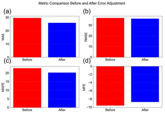
Figure 11.
Decision tree model evaluation before and after training mean percentage error adjustment; (a) mean absolute error; (b) root mean squared error; (c) mean absolute percentage error; and (d) mean percentage error.
Effect of Data Augmentation
It is well established in the literature that data augmentation is a powerful and effective tool in ML that enables small to medium datasets to attain high performance. Oh and Ki [12] trained an ML model on only three laser processing conditions that were augmented to 213 samples via sliding-window cropping, delivering an impressive 94% accuracy, significantly outperforming a physics-based carbon diffusion model (85%). Other studies have also shown the impact of data augmentation on ML model performance including KNN [13] and DT [14] models.
The dataset used in this study consists of 81 samples and can be considered small to medium in size. In general, ML models tend to perform better with larger datasets. While the dataset includes repeated measurements (n = 3) to account for experimental variability and is bounded by a well-defined 3 × 3 DOE, the addition of more intermediate data points would likely help the model capture the nonlinear characteristics of the PLAL process more effectively. However, data collection in PLAL is time-consuming, energy-intensive, and material-costly. As a result, researchers are increasingly adopting strategies, such as data augmentation or physics-informed models, to generate synthetic data that is representative of real-world observations, thereby improving model generalization. In some cases, synthetic data are deliberately used to introduce noise and challenge the model, enhancing its ability to generalize. In this work, data augmentation was explored as a strategy to improve the R2 value of the DT model used for NP size prediction.
Although model errors already fell within the acceptable range, as defined by the standard experimental error (27.2 nm), an attempt was made to further improve performance by generating synthetic data. A random sampling from a normal distribution was assumed for each experiment in order to generate the augmented data. These synthetic values sampled using the calculated means and standard deviations from the three repeated measurements. Different levels of oversampling were examined: 33.3%, 66.7%, and 100%. At 33.3% oversampling, one new synthetic sample was generated for each of the 27 experiments, resulting in 27 additional samples. At 66.7%, two new synthetic points per experiment yielded 54 additional samples, while 100% oversampling produced three synthetic data points per experiment, resulting in a total dataset of 162 entries (double the origin 81 data points).
Given the enlarged dataset, a 70:30 train–test split was used to increase the proportion of test data. Data augmentation at the 66.7% level improved model performance, as shown in Figure 12. In contrast, both 33.3% and 100% augmentation led to reductions in R2. The lower impact at 33.3% suggests insufficient new information, while 100% augmentation may have introduced excessive noise due to the high proportion of synthetic data.
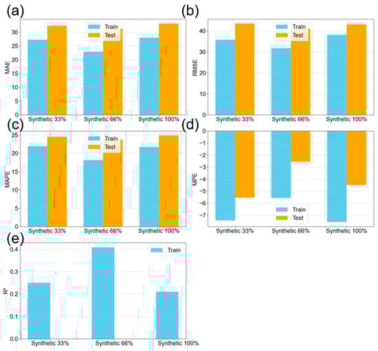
Figure 12.
Evaluation metrics of the decision tree model with synthetic data from k = 5 cross-validation showing both training and testing results for the prediction of the nanoparticle mean diameter; (a) mean absolute error; (b) root mean squared error; (c) mean absolute percentage error; (d) mean percentage error; and (e) R-squared value.
It is important to note that without k = 5 cross-validation, the model achieved higher R2 values (e.g., around 90%). However, cross-validation provides a more reliable estimate of model performance on unseen data and is, therefore, preferred. Data augmentation did not significantly reduce MAE or RMSE (Figure 12a–d), but it did lead to increased R2 (Figure 12e) and a reduction in MPE. Additionally, data augmentation at 66.7% did not alter the shape of the NP size distribution when compared to the original dataset (Figure 13a,b), although three outliers were introduced. These outliers likely arose from the random sampling process and are a known risk when generating data from probabilistic distributions. Furthermore, the addition of synthetic data increased the magnitude of correlation coefficients in the dataset, as shown in the heatmap in Figure 14 (compared to Figure 6). This allowed the model to capture stronger relationships, thereby enhancing predictive performance. Although the correlation signs remained unchanged, the magnitude increase supports the observed model improvements. Some correlations among the input features also began to emerge (although weak), consistent with expectations in PLAL, where input parameters often exhibit synergistic interactions.
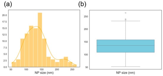
Figure 13.
(a) Histogram showing the distribution (after adding 66% synthetic data) of nanoparticle mean diameters and (b) box plot showing the distribution (after adding 66% synthetic data) of nanoparticle mean diameters.
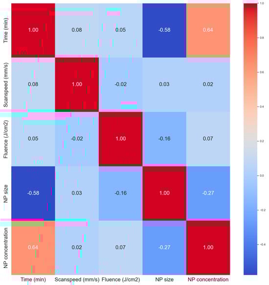
Figure 14.
Correlation matrix (heat map) of the dataset after adding 66% synthetic data.
3.3. Recommender System
Recommender systems assist users in making informed decisions. Common applications include shopping platforms, where items are recommended based on previously selected products (content-based recommenders), or streaming services, where popular content is suggested based on collective viewing trends (ranking-based recommenders). In research, recommender systems are increasingly being explored for tasks, such as material selection and, in this case, processing parameter optimization. Here, a similarity-based recommender system is developed to suggest laser processing parameters based on the user’s desired nanoparticle properties. Two systems were constructed: one using Cosine similarity and the other using KNN. Both recommenders aim to suggest processing parameters that produce a target NP mean size and concentration. To avoid bias, both outputs were normalized, ensuring equal weighting between size and concentration in the recommendation process.
XGBoost, previously identified as the optimal model for predicting NP concentration (with errors matching experimental uncertainty), and DT, the best model for predicting NP size, were used to generate synthetic datasets. Using these models, 250 and 1250 random experimental conditions were generated using Excel’s random number generator. These conditions, along with the original dataset, were used to construct two databases: a smaller one with 331 entries and a larger one with 1331 entries. The goal was to investigate the effect of database size on recommendation performance. It is important to acknowledge that the recommender system operates with constraints. Predictions are inherently limited by the accuracy of the ML models and confined within the original 3×3 DOE design space. These limitations make the recommender more realistic, as its outputs remain grounded in experimentally validated regions.
The first recommender is based on Cosine similarity, as described by Equation (10), where the most similar row from the database is recommended. The second system uses KNN with 1, 2, or 3 nearest neighbors and relies on Euclidean distance (Equation (6)) to identify similar cases. To evaluate performance, 100 random combinations of NP mean size and concentration were generated, bounded between the minimum and maximum values in the database: 53–240 nm for NP size, and 0.219–2.541 for concentration. The recommender systems were then tasked with suggesting processing parameters that yield the requested outputs. MAPE was computed between the requested and actual database values for both NP size and concentration, with results summarized in Table 6. The KNN recommender outperformed the Cosine similarity model, as shown in Table 6. This is attributed to the fact that Cosine similarity assumes outputs reside in a linearly meaningful vector space, whereas KNN, particularly with appropriate scaling, can approximate nonlinear mappings more effectively by evaluating local neighborhoods in multi-dimensional space. The KNN model achieved the best performance at k = 1; increasing the number of neighbors increased model error (MAPE).
Table 6.
Cosine similarity and KNN recommender systems evaluation.
Interestingly, increasing the database size from 331 to 1331 entries had no impact on MAPE for either recommender system. This suggests that the current database size is sufficient and that model performance may be approaching a ceiling under the constraints of the current design space. Residual plots for the NP size and concentration recommendations are shown in Figure 15a and Figure 15b, respectively. The residuals are centered around zero, indicating that the errors resemble white noise and are unlikely to be reduced through simple modeling techniques. The overall low error values and balanced performance across both outputs demonstrate that the recommender system is well-suited for real-world applications. While the addition of further data did not enhance performance within the current DOE boundaries, expanding the experimental space beyond the 3 × 3 DOE may offer new insights and further improvements in the future.
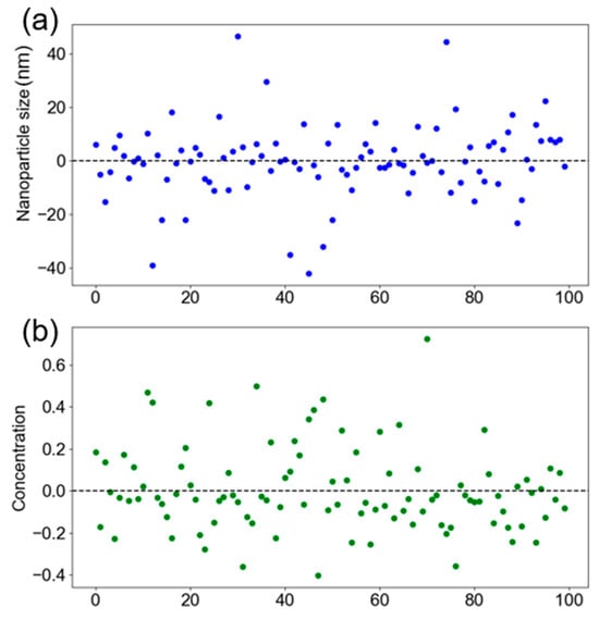
Figure 15.
KNN based recommender system residual error plot for the (a) nanoparticle size and (b) nanoparticle concentration.
The distribution of the small database (331 datapoints) is shown in Figure 16 for both NP size and concentration. The overall distribution shape remains consistent with that of the original dataset, where bimodal tendencies are observed for both output variables. However, a number of outliers are present, likely due to the extreme values introduced by the random nature of the synthetic data generation process. These outliers could potentially be reduced through additional replicate experiments in the original dataset, which would lower the standard error and increase the reliability of synthetic sampling. In the case of concentration, the boxplot identifies values around two as outliers. However, these values are known to be valid entries from the original experimental dataset and are, therefore, not considered true anomalies. The presence of outliers is likely due to the distribution of randomly generated processing parameters, which resulted in a higher concentration of predictions around 0.5 and 1. Consequently, the perceived outliers are a reflection of the sampling bias and not a significant concern for the integrity of the data. Figure 17 presents the correlation heatmap for the larger database (1331 entries). The correlation signs remain consistent with those of the original dataset, indicating that the augmented database is representative of the real experimental data. Figure 18 shows the distribution of the larger dataset, which closely mirrors that of the smaller database in Figure 16. This similarity in distribution supports the observation that database size had no impact on model performance, as reflected in the results presented in Table 6.
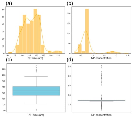
Figure 16.
Histogram showing the distribution (from the smaller database with 331 datapoints) of nanoparticle (a) mean diameters and (b) concentration. Box plot showing the distribution (from the smaller database with 331 datapoints) of nanoparticle (c) mean diameters and (d) concentration.
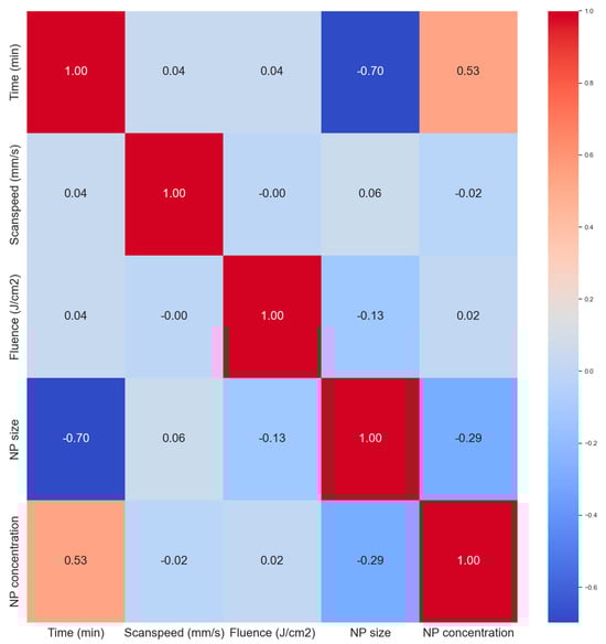
Figure 17.
Correlation matrix (heat map) of the dataset after making 1250 predictions using decision tree model (for nanoparticle size) and XGBoost (for nanoparticle concentration).
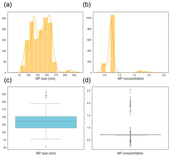
Figure 18.
Histogram showing the distribution (from the final database with 1331 datapoints) of nanoparticle (a) mean diameters, and (b) concentration. Box plot showing the distribution (from the final database with 1331 datapoints) of nanoparticle (c) mean diameters, and (d) concentration.
4. Recommendations
The recommender system can be further validated through more physical experimentation. By conducting new experiments guided by the system’s recommendations, especially within the existing 3 × 3 DOE zone—it is possible to assess its predictive accuracy under real conditions. The current design space already spans a wide range of NP sizes (52–240 nm), which is sufficient for many practical applications. However, further optimization could focus on identifying processing parameters that achieve similar results while minimizing resource usage, for example, reducing ablation time or laser fluence. These refinements would contribute to more sustainable manufacturing, an important consideration for industrial applications where PLAL may operate continuously. In such scenarios, energy efficiency and throughput become more critical than in laboratory-scale research.
To test the system’s robustness, a selection of 10 randomly generated NP property combinations could be physically tested. This would enable further comparison between predicted and experimental outcomes. Additionally, the model could be challenged to predict outside the established DOE boundaries—such as producing NP sizes below 50 nm or above 240 nm, and concentrations beyond current experimental limits. These extrapolations, guided by AI, could lead to the discovery of new, high-performance nanoparticle formulations.
As the system is tested in these uncharted regions, the model can continue to evolve, learning from prediction errors and refining its recommendations over time. Even unsuccessful experiments will contribute valuable information to the database, incrementally improving the model’s accuracy and efficiency. Compared to traditional trial-and-error or fixed DOE strategies, this adaptive, AI-driven approach could significantly accelerate the discovery of optimal laser processing parameters.
Another potential avenue for future work is testing the system with different materials. At initial deployment, performance may be suboptimal if the new material significantly differs from magnesium in properties such as starting powder particle size or laser absorption at 1064 nm. Nonetheless, this approach could serve as the foundation for building a broader, open-access database for PLAL across materials. Such a system would help transition PLAL from a laboratory-scale technique to an industrial-scale solution by mitigating the complexity of parameter selection and improving consistency in NP yield and quality. The recommender system can be adapted to other materials, starting with those that share similar properties with magnesium, such as metal oxides. This extension will require additional experiments using these materials. To further accelerate prediction and reduce the number of required experiments—especially when working with new materials—a physics-informed model can be incorporated. Such a model would leverage material-specific properties, including density, absorption at the laser wavelength, powder particle size, crystal structure, melting point, boiling point, and others. Integrating this physics-informed layer would enhance the system’s generalizability and efficiency across a broader range of materials.
Further investigation into additional PLAL parameters, such as the liquid medium (IPA was used in this study) or laser repetition rate (fixed at 10 kHz), is also recommended. With appropriate calibration, the recommender system architecture developed here could be extended to different laser systems. In the long term, the recommender system or its framework could support the creation of open-access dashboards or mobile applications, allowing researchers to bypass years of manual data generation and focus on applying NPs in advanced domains such as sensing, Mg-ion batteries, or cancer therapy. Magnesium nanoparticles are widely recognized for their potential in various advanced applications, including sensing [19], battery anode fabrication [20], and antimicrobial material [21]. In each of these domains, there exists an optimal NP size–concentration combination that directly influences the performance and efficiency of the application. For example, smaller NPs may enhance surface reactivity in sensors or improve diffusion in antimicrobial applications, while larger or more concentrated NPs may be preferable for specific energy storage requirements. This study demonstrates that such application-specific NP targets can be integrated into the recommender system, enabling users to input the desired end-use scenario (e.g., antimicrobial or Mg-ion batteries). The system can then suggest optimal PLAL processing parameters that produce the appropriate NP size and concentration for that particular application. This functionality significantly enhances the practicality and usability of PLAL-based synthesis, moving it closer to tailored, on-demand, automated NP production guided by artificial intelligence.
On another note, in this study, NP mean size was measured via DLS. Various metrics exist for reporting NP size in colloids, including Mean Intensity Diameter, Mean Volume Diameter, Mean Area Diameter, and Mean Number Diameter. The Mean Intensity Diameter is heavily influenced by larger particles due to the dependence on light scattering intensity. Mean Volume Diameter accounts for particle volume, still favoring larger particles, albeit less so. Mean Area Diameter weights by surface area, offering a more balanced representation. Mean Number Diameter, which gives equal weight to all particle sizes, is the most commonly reported metric in the literature and tends to produce lower values than other methods. Therefore, this method was adopted and used consistently throughout this work. In future studies, ML models could be developed to account for multiple NP size metrics simultaneously, enabling a more comprehensive understanding of particle size distributions. A recommender system that integrates multiple measurement approaches could further enhance robustness and provide a more complete representation of colloidal characteristics beyond a single average size.
Another important avenue for future work is the prediction of nanoparticle (NP) size distribution metrics, such as the full width at half maximum (FWHM) or its half-width. This task will involve applying and evaluating various machine learning algorithms—similar to the approach used for predicting NP size and concentration—to identify the optimal model. Incorporating this capability will enhance the recommender system’s comprehensiveness and increase the specificity of its recommendations. Additionally, further predictive variables can be integrated into the system, including the viscosity of the colloid, its electrical conductivity in liquid form, and the Zeta potential, which serves as an indicator of colloidal stability. The crystal structure of the Mg NPs can also be investigated using techniques such as X-ray Diffraction (XRD) and/or Electron Backscatter Diffraction (EBSD). Measurements and recordings from these techniques can be collected to build a dataset for predicting the crystal structure of the resulting nanoparticles. Incorporating this information further enhances the recommender system, making it more comprehensive and informative. The system could be designed with a user interface that allows users to select the specific properties that are critical for their application—for example, size and crystal structure, or size and Zeta potential. As more user-defined requirements are added, the system can generate more precisely tailored nanoparticle inks optimized for the intended application. Furthermore, future work should include a detailed analysis of time-based measurements, such as the 10 Dynamic Light Scattering (DLS) runs per sample, to investigate temporal drift or fluctuations across measurements. Techniques, such as autocorrelation analysis or variance-over-time assessments, will be valuable in determining the stability and reliability of the DLS data, thereby improving the accuracy of size-related predictions in the recommender system.
5. Conclusions
The three key conclusions from this research article are as follows:
- Research Question and Gap: The study addressed the lack of machine learning-based, data-driven methods for selecting Pulsed laser ablation in liquid (PLAL) parameters to control nanoparticle (NP) size and concentration combinations. This area historically driven by trial-and-error and DOE methods, which limits practical and industrial applications of the technology. There was not a direct comparison of the developed recommender system with literature examples since this is the first article to propose such approach.
- Approach and Models Used: seven machine learning models, including K-Nearest Neighbors (KNN), Extreme Gradient Boosting (XGBoost), Support Vector Regressor, Random Forest, Decision trees (DT), Multiple linear regression, and Multiple Polynomial regression, were developed and compared to predict NP properties and enable a recommender system. The DT model achieved the best performance for predicting the NP size with the XGBoost model achieved the best performance for predicting the NP concentration. The XGBoost model attained a competitive mean percentage error (MPE) of 2% for NP concentration while the DT model attained an MPE of 10% for NP size prediction. The optimized recommender system based on KNN attained a MPAE of 8% and 29% for NP size and concentration, respectively.
- Recommendations: The model is ready for deployment in physical experiments. Future work will involve extrapolation beyond the design space (targeting beyond 52–240 nm range explored herein), and adaptation to other materials other than magnesium.
Author Contributions
Conceptualization, A.N. and D.B.; Software, A.N.; Validation, A.N. and D.B.; Investigation, A.N.; Writing—original draft, A.N.; Writing—review & editing, A.N. and D.B.; Visualization, A.N.; Supervision, D.B.; Funding acquisition, D.B. All authors have read and agreed to the published version of the manuscript.
Funding
This research was funded by Research Ireland and the European Regional Development Fund, grant number 21/RC/10295_P2 and the APC was funded by Dublin City University.
Data Availability Statement
The raw data supporting the conclusions of this article will be made available by the authors on request.
Acknowledgments
For the purpose of Open Access, the author has applied a CC BY public copyright license to any Author Accepted Manuscript version arising from this submission. This work is supported by I-Form. The material characterization was carried out at the Nano Research Facility in Dublin City University which was funded under the Programme for Research in Third Level Institutions (PRTLI) Cycle 5. The PRTLI is co-funded through the European Regional Development Fund (ERDF), part of the European Union Structural Funds Programme 2011–2015.
Conflicts of Interest
The authors declare that they have no known competing financial interests or personal relationships that could have appeared to influence the work reported in this paper.
References
- Guillén, G.G.; Zuñiga Ibarra, V.A.; Mendivil Palma, M.I.; Krishnan, B.; Avellaneda, D.A.; Shaji, S. Effects of Liquid Medium and Ablation Wavelength on the Properties of Cadmium Sulfide Nanoparticles Formed by Pulsed-Laser Ablation. Chem. Phys. Chem. 2017, 18, 1035–1046. [Google Scholar] [CrossRef] [PubMed]
- Al-Hamaoy, A.; Chikarakara, E.; Jawad, H.; Gupta, K.; Kumar, D.; Rao, M.S.R.; Krishnamurthy, S.; Morshed, M.; Fox, E.; Brougham, D.; et al. Liquid Phase-Pulsed Laser Ablation: A route to fabricate different carbon nanostructures. Appl. Surf. Sci. 2014, 302, 141–144. [Google Scholar] [CrossRef]
- Saraj, C.S.; Singh, S.C.; Verma, G.; Alquliah, A.; Li, W.; Guo, C. Rapid fabrication of CuMoO4 nanocomposites via electric field assisted pulsed-laser ablation in liquids for electrochemical hydrogen generation. Appl. Surf. Sci. Adv. 2023, 13, 100358. [Google Scholar] [CrossRef]
- Hahn, A.; Barcikowski, S.; Chichkov, B.N. Influences on nanoparticle production during pulsed laser ablation. J. Laser Micro Nanoeng. 2007, 3, 73–77. [Google Scholar] [CrossRef]
- Pereira, H.; Moura, C.G.; Miranda, G.; Silva, F.S. Influence of liquid media and laser energy on the production of MgO nanoparticles by laser ablation. Opt. Laser Technol. 2021, 142, 107181. [Google Scholar] [CrossRef]
- Attallah, A.H.; Abdulwahid, F.S.; Ali, Y.A.; Haider, A.J. Effect of Liquid and Laser Parameters on Fabrication of Nanoparticles via Pulsed Laser Ablation in Liquid with Their Applications: A Review. Plasmon. 2023, 18, 1307–1323. [Google Scholar] [CrossRef]
- Fazio, E.; Gökce, B.; De Giacomo, A.; Meneghetti, M.; Compagnini, G.; Tommasini, M.; Waag, F.; Lucotti, A.; Zanchi, C.G.; Ossi, P.M.; et al. Nanoparticles Engineering by Pulsed Laser Ablation in Liquids: Concepts and Applications. Nanomaterials 2020, 10, 2317. [Google Scholar] [CrossRef] [PubMed]
- Khairani, I.Y.; Mínguez-Vega, G.; Doñate-Buendía, C.; Gökce, B. Green nanoparticle synthesis at scale: A perspective on overcoming the limits of pulsed laser ablation in liquids for high-throughput production. Phys. Chem. Chem. Phys. 2023, 25, 19380–19408. [Google Scholar] [CrossRef] [PubMed]
- Tsai, C.C.; Yiu, T.H. Investigation of Laser Ablation Quality Based on Data Science and Machine Learning XGBoost Classifier. Appl. Sci. 2024, 14, 326. [Google Scholar] [CrossRef]
- Hussein, M.M.; Mutlag, H.; Shareef, H. Optimization of an artificial neural network to estimate laser ablation efficiency. Laser Phys. 2019, 29, 115603. [Google Scholar] [CrossRef]
- Wang, B.; Wang, P.; Song, J.; Lam, Y.C.; Song, H.; Wang, Y.; Liu, S. A hybrid machine learning approach to determine the optimal processing window in femtosecond laser-induced periodic nanostructures. J. Mater. Process Technol. 2022, 308, 117716. [Google Scholar] [CrossRef]
- Oh, S.; Ki, H. Deep learning model for predicting hardness distribution in laser heat treatment of AISI H13 tool steel. Appl. Therm. Eng. 2019, 153, 583–595. [Google Scholar] [CrossRef]
- Chaudhari, P.; Agarwal, H.; Bhateja, V. Data augmentation for cancer classification in oncogenomics: An improved KNN based approach. Evol. Intell. 2021, 14, 489–498. [Google Scholar] [CrossRef]
- Juwara, L.; El-Hussuna, A.; El Emam, K. An evaluation of synthetic data augmentation for mitigating covariate bias in health data. Patterns 2024, 5, 100946. [Google Scholar] [CrossRef] [PubMed]
- Park, J.; Kim, Y.M.; Hong, S.; Han, B.; Nam, K.T.; Jung, Y. Closed-loop optimization of nanoparticle synthesis enabled by robotics and machine learning. Matter 2023, 6, 677–690. [Google Scholar] [CrossRef]
- Bakhtiyari, A.N.; Wang, Z.; Wang, L.; Zheng, H. A review on applications of artificial intelligence in modeling and optimization of laser beam machining. Opt. Laser Technol. 2021, 135, 106721. [Google Scholar] [CrossRef]
- Shao, W.; Lin, X.; Huang, Y.; Qu, L.; Zhuo, W.; Liu, H. Effect of Kernel Functions on the Performance of Support Vector Regression Algorithm in Predicting Patient-Specific Organ Doses from CT Scans. Radiat. Sci. Technol. 2025, 11, 1–11. [Google Scholar] [CrossRef]
- Wang, Z.; Xu, H.; Xia, L.; Zou, Z.; Soares, C.G. Kernel-based support vector regression for nonparametric modeling of ship maneuvering motion. Ocean. Eng. 2020, 216, 107994. [Google Scholar] [CrossRef]
- Shanawad, S.S.; Chethan, B.; Prasad, V.; Sunilkumar, A.; Veena, V.S. Humidity sensing performance of the magnesium oxide nanoparticles. J. Mater. Sci. Mater. Electron. 2023, 34, 244. [Google Scholar] [CrossRef]
- Sosnin, I.M.; Akimov, E.G.; Merson, E.D.; Golovanov, A.A.; Merson, D.L.; Kostin, V.I.; Linderov, M.L. Magnesium nanoparticles as a highly stable anode for the electrochemical cell. Mater. Sci. Eng. B 2023, 296, 116648. [Google Scholar] [CrossRef]
- Fouda, A.; Eid, A.M.; Abdel-Rahman, M.A.; EL-Belely, E.F.; Awad, M.A.; Hassan, S.E.D.; AL-Faifi, Z.E.; Hamza, M.F. Enhanced Antimicrobial, Cytotoxicity, Larvicidal, and Repellence Activities of Brown Algae, Cystoseira crinita-Mediated Green Synthesis of Magnesium Oxide Nanoparticles. Front. Bioeng. Biotechnol. 2022, 10, 849921. [Google Scholar] [CrossRef] [PubMed]
Disclaimer/Publisher’s Note: The statements, opinions and data contained in all publications are solely those of the individual author(s) and contributor(s) and not of MDPI and/or the editor(s). MDPI and/or the editor(s) disclaim responsibility for any injury to people or property resulting from any ideas, methods, instructions or products referred to in the content. |
© 2025 by the authors. Licensee MDPI, Basel, Switzerland. This article is an open access article distributed under the terms and conditions of the Creative Commons Attribution (CC BY) license (https://creativecommons.org/licenses/by/4.0/).