
Optimization of ATIG Weld Based on a Swarm Intelligence Approach: Application to the Design of Welding in Selected Manufacturing Processes


Abstract
1. Introduction
- -
- -
2. Materials and Methods
2.1. Materials
2.2. Welding Procedure
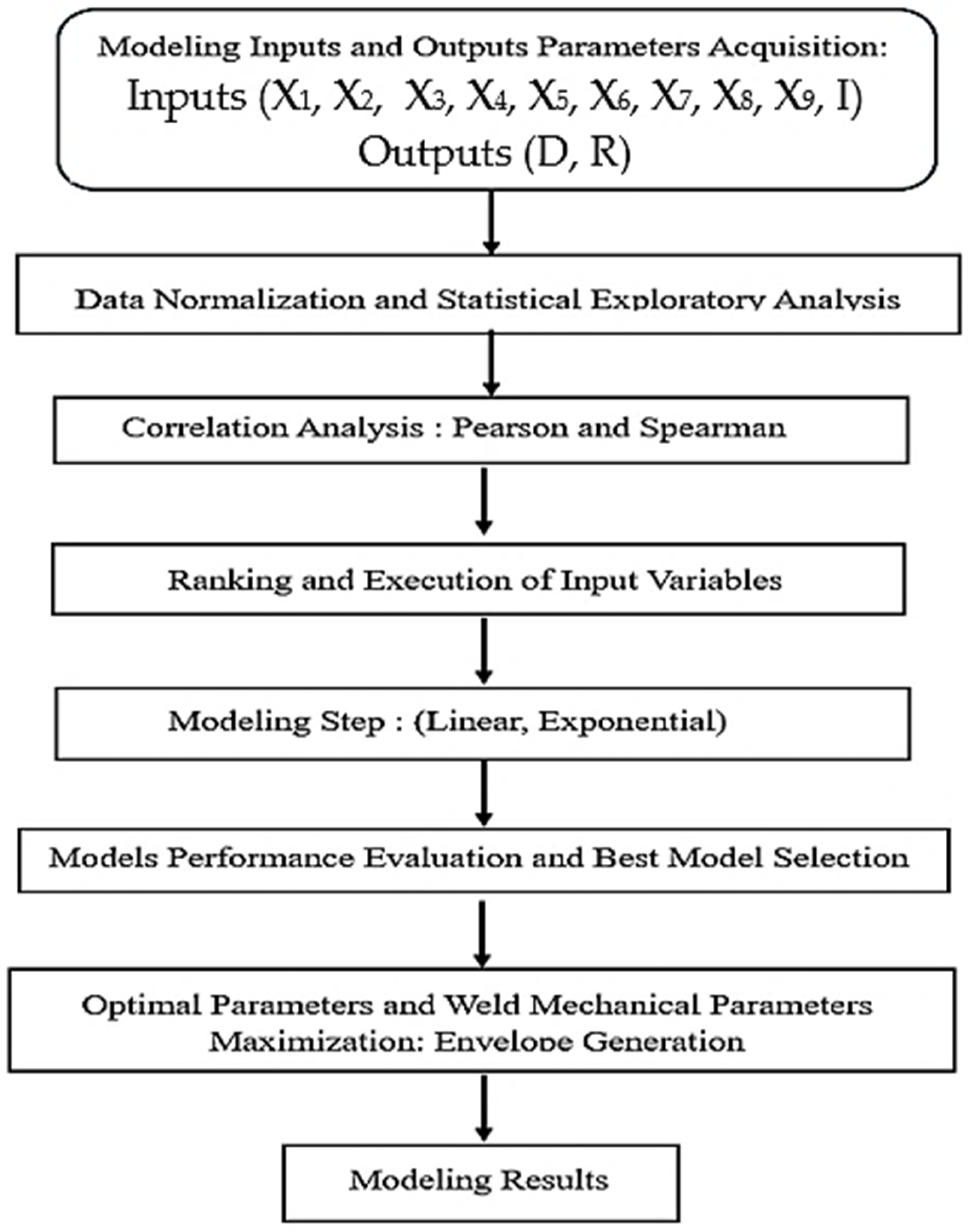
2.3. Methodology
- Initialization: A swarm (group) of particles is initialized randomly inside an interval ranging from the lower limit to the upper limit of the coefficient. However, random initialization may be replaced by manual initialization if the user has an idea about the coefficient’s probable value. In PSO, each particle represents a potential solution of the optimization problem coded as the particle position.
- Fitness Evaluation: The fitness of each particle is evaluated based on an objective function, such as the mean squared error (MSE) between the welding process model’s predicted outputs and the actual observed outputs.
- Update Personal Best and Global Best: Each particle keeps records of its personal best position (“P”) and the swarm collectively maintains a global best position (“G”) based on the best fitness values achieved. During the search process, each process tends to imitate the global best particle among the swarm and to track its previous best discoveries if no improved position is found.
- Velocity and Position Update: Each particle updates its velocity and position based on its personal best, the global best, and its current velocity. The particle moves equations involve three components: current velocity, past own visited position, and the position of the global best particle. Based on this combination, each particle illustrates the social behavior and the cognitive behavior.
- Iteration: The optimization process is repeated for a preset number of iterations until a convergence criterion is met, such as when the change in global best fitness value falls below a threshold or if there is no improvement in the discovered solution for a certain number of iterations. Those conditions are usually known as the possible stopping criteria.
- Output: After stopping, the PSO algorithm provides the global best position (position of the global best particle among the swarm), which represents the optimized model coefficients of the welding process.
- is the velocity of particle i at iteration k.
- is the inertia weight for controlling the impact of the previous velocity.
- are the acceleration coefficients for cognitive and social components.
- , are the random numbers uniformly distributed in [0, 1].
- is the best position of particle i.
- is the global best position.
- is the current position of particle i.
- is the observed output for the j-th data point.
- is the model-predicted output for the j-th data point given the coefficients .
- n is the number of data points.
3. Results and Discussions
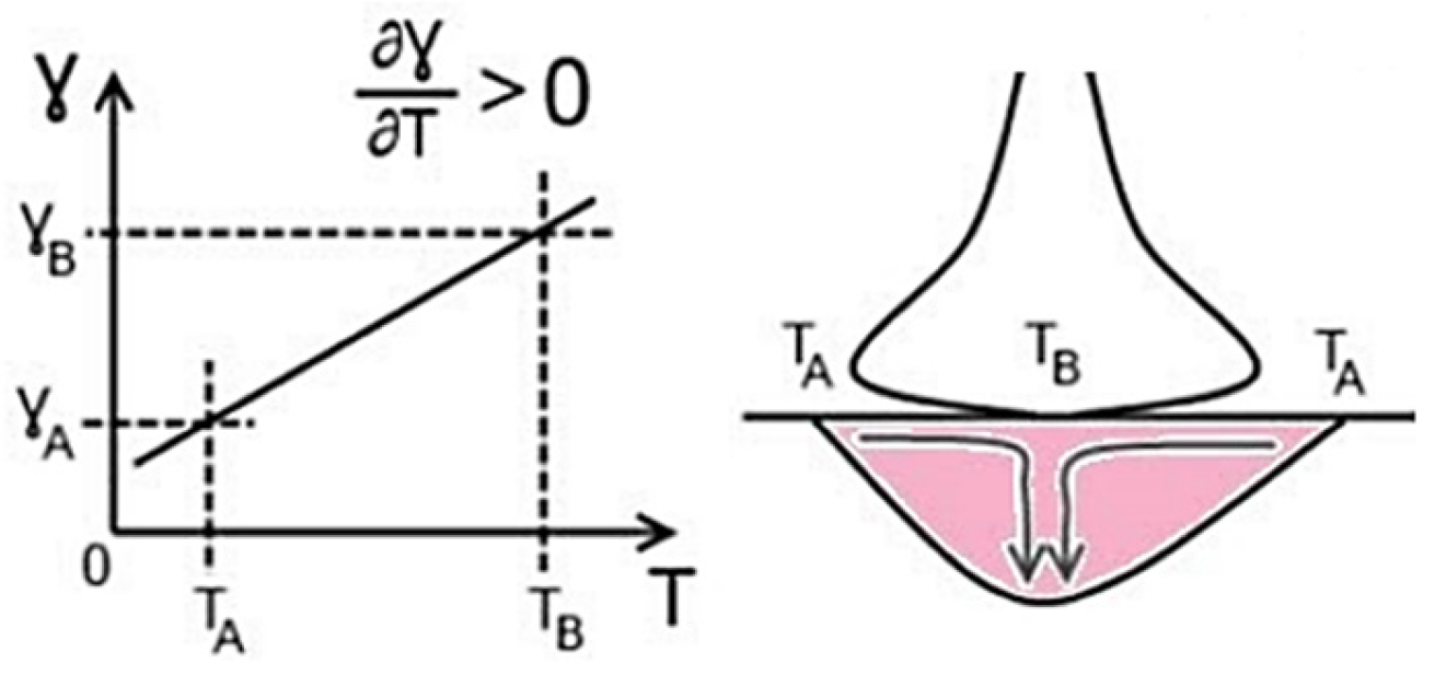
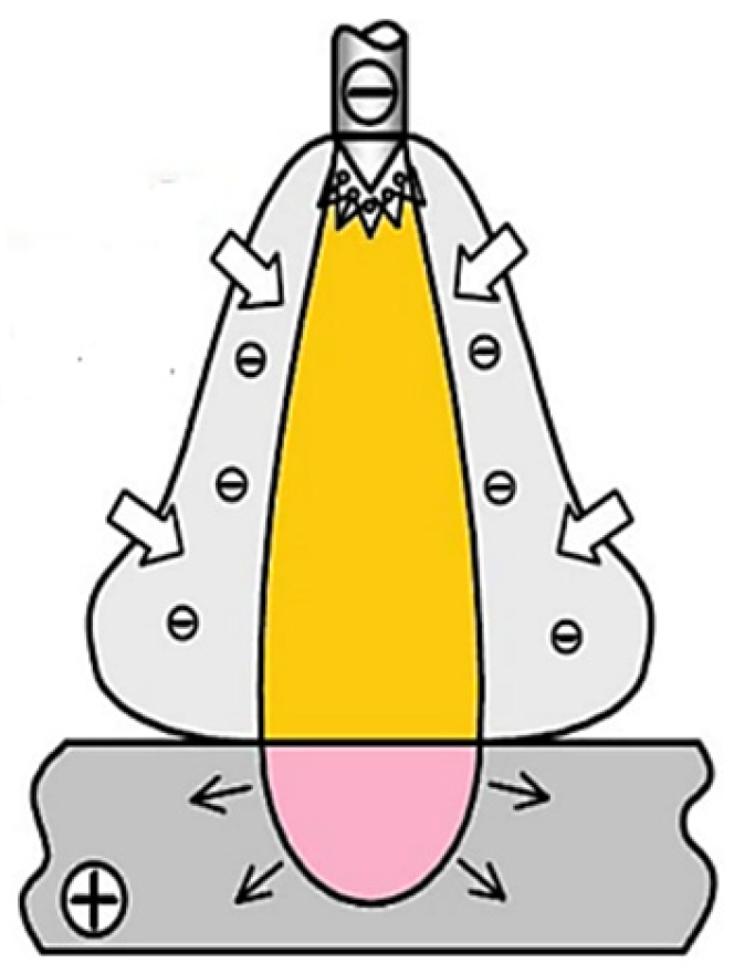
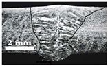
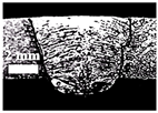
3.1. Weld Morphology
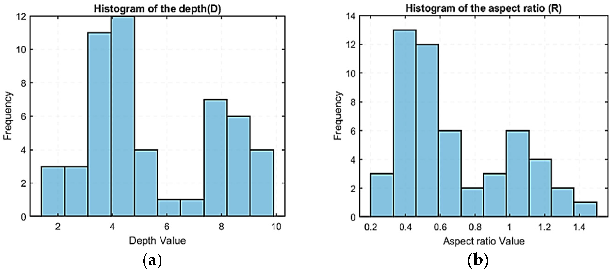
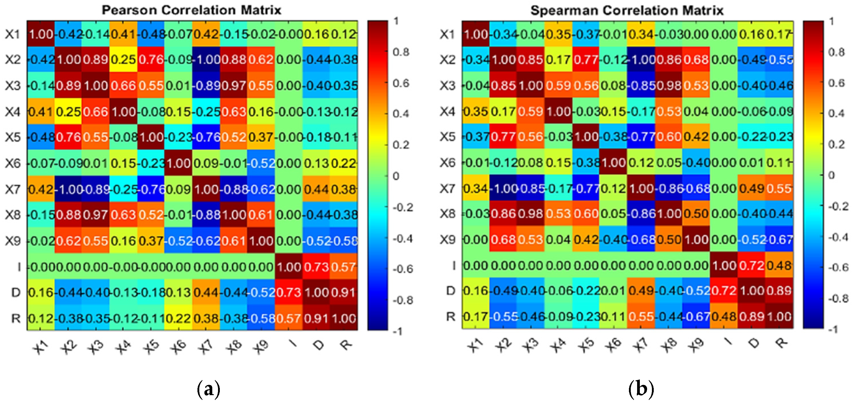
3.2. Statistical Exploratory Analysis and Correlation Study
3.3. Models’ Development
3.4. Application to a Design Problem
4. Conclusions
Author Contributions
Funding
Data Availability Statement
Conflicts of Interest
References
- Nouri, A.; Wen, C. Stainless steels in orthopedics. In Structural Biomaterials—Properties, Characteristics and Selection, Woodhead Publishing Series in Biomaterials; Woodhead Publishing: Cambridge, UK, 2021; pp. 67–101. [Google Scholar]
- Singh, C.; Lee, T.; Lee, K.H.; Kim, Y.S.; Huang, E.-W.; Jain, J.; Liaw, P.K.; Lee, S.Y. Exceptional fatigue-resistant austenitic stainless steel for cryogenic applications. Appl. Mater. Today 2024, 38, 102195. [Google Scholar] [CrossRef]
- Fashu, S.; Trabadelo, V. A critical review on development, performance and selection of stainless steels and nickel alloys for the wet phosphoric acid process. Mater. Des. 2023, 227, 111739. [Google Scholar] [CrossRef]
- Gary, S.W.; Shigeharu, U. Structural Alloys for Nuclear Energy Applications, Chapter 8—Austenitic Stainless Steels; Odette, G.R., Zinkle, S.J., Eds.; Elsevier: Amsterdam, The Netherlands, 2019; pp. 293–347. [Google Scholar]
- Leconte, S.; Paillard, P.; Chapelle, P.; Henrion, G.; Saindrenan, J. Effect of oxide fluxes on activation mechanisms of tungsten inert gas process. Sci. Techno. Weld. Join. 2006, 11, 389–397. [Google Scholar] [CrossRef]
- Patel, N.P.; Sharma, D.K.; Upadhyay, G.H. Effect of Activated Fluxes on Weld Penetration and Mechanism Responsible for Deeper Penetration of Stainless Steels—A Review. In Current Advances in Mechanical Engineering; Lecture Notes in Mechanical Engineering (LNME); Springer: Singapore, 2021; pp. 737–746. [Google Scholar]
- Aljufri, A.; Sofyan, S.; Muhammad, R.; Reza, P.; Indra, M. Influence of shielding gas flow on the TIG welding process using stainless steel 304 material. J. Weld. Tech. 2024, 6, 38–45. [Google Scholar] [CrossRef]
- Kim, I.-S.; Lee, M.-G.; Jeon, Y. Review on Machine Learning Based Welding Quality Improvement. Int. J. Precis. Eng. Manuf.-Smart Technol. 2023, 1, 219–226. [Google Scholar] [CrossRef]
- Mahadevan, R.R.; Jagan, A.; Pavithran, L.; Shrivastava, A.; Selvaraj, S.K. Intelligent welding by using machine learning techniques. Mater. Today Proc. 2021, 26, 7402–7410. [Google Scholar] [CrossRef]
- Srinivasan, D.; Sevvel, P.; Dhanesh, B.S.D.; Vasanthe, R. Optimization of parameters and formulation of numerical model employing GRA–PCA and RSM approach for friction stir welded Ti–6Al–4V alloy joints. Mater. Res. Express 2024, 11, 056511. [Google Scholar] [CrossRef]
- John Solomon, I.; Sevvel, P.; Gunasekaran, J.; Vasanthe Roy, J. Parametric-based optimization of friction stir welded wrought AZ80A Mg alloy employing response surface methodology. Mater. Res. Express 2023, 10, 116514. [Google Scholar] [CrossRef]
- Tesfaye, F.K.; Getaneh, A.M. The grey-based Taguchi method was used to enhance the TIG-MIG hybrid welding process parameters for mild steel. Invent. Discl. 2024, 4, 100016. [Google Scholar] [CrossRef]
- Abima, C.S.; Akinlabi, S.A.; Madushele, N.; Fatoba, O.S.; Akinlabi, E.T. Multi-objective optimization of process parameters in TIG-MIG welded AISI 1008 steel for improved structural integrity. Int. J. Adv. Manuf. Technol. 2021, 118, 3601–3615. [Google Scholar] [CrossRef]
- Choudhury, B.; Chandrasekaran, M.; Devarasiddappa, D. Development of ANN modeling for estimation of weld strength and integrated optimization for GTAW of Inconel 825 sheets used in aero engine components. J. Braz. Soc. Mech. Sci. Eng. 2020, 42, 308. [Google Scholar] [CrossRef]
- Ghosh, N. Effect of GTAW process parameters on AISI 304L austenitic stainless steels and optimization using Grey-Taguchi technique. Can. Metall. Q. 2024, 1–10. [Google Scholar] [CrossRef]
- Adirek, B.; Wasawat, N.; Nuttachat, W. Optimization of Tungsten Inert Gas Welding Process Parameters for AISI 304 Stainless Steel. Defect Diffus. Forum 2022, 417, 23–28. [Google Scholar]
- Pratheesh, K.S.; Anand, K.; Rajesh, R.; Ashwin, S. Optimization of Tungsten Inert Gas Welding Process Parameters on AA6013. In Materials, Design, and Manufacturing for Sustainable Environment; Lecture Notes in Mechanical Engineering(LNME); Springer: Singapore, 2022; pp. 381–396. [Google Scholar] [CrossRef]
- Vora, J.J.; Abhishek, K.; Srinivasan, S. Attaining optimized A-TIG welding parameters for carbon steels by advanced parameter-less optimization techniques: With experimental validation. J. Braz. Soc. Mech. Sci. Eng. 2019, 41, 261. [Google Scholar] [CrossRef]
- Ghumman, K.Z.; Ali, S.; Khan, N.B.; Khan, M.H.; Ali, H.T.; Ashurov, M. Optimization of TIG welding parameters for enhanced mechanical properties in AISI 316L stainless steel welds. Int. J. Adv. Manuf. Technol. 2025, 136, 353–365. [Google Scholar] [CrossRef]
- Hedhibi, A.C.; Touileb, K.; Djoudjou, R.; Ouis, A.; Alrobei, H.; Ahmed, M.M.Z. Mechanical Properties and Microstructure of TIG and ATIG Welded 316L Austenitic Stainless Steel with Multi-Components Flux Optimization Using Mixing Design Method and Particle Swarm Optimization (PSO). Materials 2021, 14, 7139. [Google Scholar] [CrossRef] [PubMed]
- Sivakumar, J.; Vasudevan, M.; Korra, N.N. Systematic Welding Process Parameter Optimization in Activated Tungsten Inert Gas (A-TIG) Welding of Inconel 625. Trans. Indian Inst. Met. 2022, 73, 555–569. [Google Scholar] [CrossRef]
- Kumaar, S.S.; Korra, N.N.; Devakumaran, K.; Kumar, G. Optimization of Process Parameters for the A-TIG Welding of Inconel 617 using Particle Swarm Optimization (PSO) and Genetic Algorithm (GA). Surf. Rev. Lett. 2022, 29, 2250136. [Google Scholar] [CrossRef]
- Sivakumar, J.; Korra, N.N. Optimization of Welding Process Parameters for Activated Tungsten Inert Welding of Inconel 625 Using the Technique for Order Preference by Similarity to Ideal Solution Methodology. Arab. J. Sci. Eng. 2021, 46, 7399–7409. [Google Scholar] [CrossRef]
- Sekar, C.B.; Boopathy, S.R.; Vijayan, S.R.; Rao, S.R.K. Multi-objective optimization of welding parameters using Taguchi-based grey relation analysis in activated TIG(ATIG), welding on SAF2507 super duplex stainless steel. AIP Conf. Proc. 2021, 2395, 30007. [Google Scholar] [CrossRef]
- Vuherer, T.; Bajić, D.; Manjgo, M.; Bjelajac, E.; Skumavc, A.; Orožim, U.; Lojen, G. Comparison of ATIG welding powders and their influence on mechanical properties. Zavar. I Zavarene Konstr. 2024, 69, 99–110. [Google Scholar] [CrossRef]
- Mills, K.C. Recommended Values of Thermophysical Properties for Selected Commercial Alloys; National Physical Laboratory 472 and ASM International; Woodhead Publishing Limited: Cambridge, UK, 2002. [Google Scholar]
- Cabello-Solorzano, K.; Ortigosa de Araujo, I.; Peña, M.; Correia, L.; Tallón-Ballesteros, A.J. The Impact of Data Normalization on the Accuracy of Machine Learning Algorithms: A Comparative Analysis. In Proceedings of the 18th International Conference on Soft Computing Models in Industrial and Environmental Applications (SOCO 2023), Salamanca, Spain, 5–7 September 2023; Springer: Cham, Switzerland, 2023; Volume 750, pp. 344–353. [Google Scholar] [CrossRef]
- Singh, D.; Singh, B. Feature-wise normalization: An effective way of normalizing data. Pattern Recognit. 2022, 122, 108307. [Google Scholar] [CrossRef]
- de Winter, J.C.F.; Gosling, S.D.; Potter, J. Comparing the Pearson and Spearman correlation coefficients across distributions and sample sizes: A tutorial using simulations and empirical data. Psychol. Methods 2016, 21, 273–290. [Google Scholar] [CrossRef] [PubMed]
- Azadi Moghaddam, M.; Kolahan, F. Optimization of A-TIG Welding Process Using Simulated Annealing Algorithm. J. Adv. Manuf. Syst. 2020, 19, 869–891. [Google Scholar] [CrossRef]
- Pu, Y.; Rong, Y.; Chen, J.; Mao, Y. Accelerated Identification Algorithms for Exponential Nonlinear Models: Two-Stage Method and Particle Swarm Optimization Method. Circuits Syst. Signal Process. 2022, 41, 2636–2652. [Google Scholar] [CrossRef]
- Kozinski, O.; Kotyrba, M.; Volna, E. Improving the production efficiency based on algorithmization of the planning process. Appl. Syst. Innov. 2023, 6, 77. [Google Scholar] [CrossRef]
- Touileb, K.; Djoudjou, R.; Ouis, A.; Hedhibi, A.C.; Boubaker, S.; Ahmed, M.M.Z. Particle Swarm Method for Optimization of ATIG Welding Process to Joint Mild Steel to 316L Stainless Steel. Crystals 2023, 13, 1377. [Google Scholar] [CrossRef]
- Wu, J.; Azarm, S. Metrics for quality assessment of a multiobjective design optimization solution set. J. Mech. Des. 2001, 123, 18–25. [Google Scholar] [CrossRef]
- Poblano-Salas, C.D.; Barceinas-Sanchez, J.D.O.; Sanchez-Jimenez, J.C. Failure analysis of an AISI 410 stainless steel airfoil in a steam turbine. Eng. Fail. Anal. 2011, 18, 68–74. [Google Scholar] [CrossRef]
- Mishra, A. Automotive Materials: An Overview. Int. Res. J. Eng. Technol. (IRJET) 2020, 7, 4852–4857. [Google Scholar]
- Liu, J.; Cheng, Y.; Jing, X.; Liu, X.; Chen, Y. Prediction and optimization method for welding quality of components in ship construction. Sci. Rep. 2024, 14, 9353. [Google Scholar] [CrossRef] [PubMed]
- Date, C.J. Denormalization. In Database Design and Relational Theory; Apress: Berkeley, CA, USA, 2019; pp. 161–182. [Google Scholar] [CrossRef]


| Elements | C | Mn | P | S | Si | Cr | Ni | N |
|---|---|---|---|---|---|---|---|---|
| 316L SS-Weight % | 0.03 | 2 | 0.045 | 0.003 | 0.75 | 17.5 | 8 | 0.1 |
| Melting point (°C) [26] | 1440 | |||||||
| Oxides | Enthalpy Energy (kJ/mol) | Oxides Melting Point (°C) | Oxides Boiling Point (°C) | Oxide Surface Tension (mN/m) | Oxides’ First Ionization Energy (eV) |
|---|---|---|---|---|---|
| SiO2 | −911 | 1626 | 2950 | 260 | 11.89 |
| TIO2 | −941 | 1892 | 2972 | 360 | 11.13 |
| Fe2O3 | −824 | 1540 | 1987 | 300 | 12.10 |
| Cr2O3 | −1128 | 2330 | 3000 | 800 | 11.00 |
| ZnO | −350 | 1975 | 2360 | 550 | 11.36 |
| Mn2O3 | −971 | 940 | 1080 | 310 | 10.49 |
| V2O5 | −1550.6 | 670 | 1750 | 80 | 10.12 |
| MoO3 | −745 | 802 | 1155 | 70 | 11.51 |
| Co3O4 | −577 | 1935 | 2800 | 800 | 10.95 |
| SrO | −592 | 2531 | 3200 | 600 | 11.36 |
| ZrO2 | −1080 | 2715 | 4300 | 400 | 11.90 |
| CaO | −635 | 2615 | 2850 | 625 | 10.29 |
| MgO | −602 | 2826 | 3600 | 635 | 9.43 |
| Parameters | Range |
|---|---|
| Current intensity | 120, 150, 180, 200 A |
| Welding speed | 15 cm/min |
| Electrode tip angle | 45° |
| Electrode diameter | 3.2 mm |
| Arc length Torch angle | 2 mm 90° |
| Shielding gas: Argon | 10 L/min |
| Shielding gas back: Argon | 8 L/min |
| Oxides | Oxides’ Input Parameters | ||||||||
|---|---|---|---|---|---|---|---|---|---|
| X1 | X2 | X3 | X4 | X5 | X6 | X7 | X8 | X9 | |
| SiO2 | −911 | 1626 | 2950 | 1324 | 260 | 11.89 | 1235 | 1550 | 226 |
| TIO2 | −941 | 1892 | 2972 | 1080 | 360 | 11.13 | 969 | 1572 | 492 |
| Fe2O3 | −824 | 1540 | 1987 | 447 | 300 | 12.10 | 1321 | 587 | 140 |
| Cr2O3 | −1128 | 2330 | 3000 | 670 | 800 | 11.00 | 531 | 1600 | 930 |
| ZnO | −350 | 1975 | 2360 | 385 | 550 | 11.36 | 886 | 960 | 575 |
| Mn2O3 | −971 | 940 | 1080 | 140 | 310 | 10.49 | 1921 | 320 | 460 |
| V2O5 | −1550.6 | 670 | 1750 | 1080 | 80 | 10.12 | 2192 | 350 | 730 |
| MoO3 | −745 | 802 | 1155 | 353 | 70 | 11.51 | 2059 | 245 | 598 |
| Co3O4 | −577 | 1935 | 2800 | 865 | 800 | 10.95 | 926 | 1400 | 535 |
| SrO | −592 | 2531 | 3200 | 669 | 600 | 11.36 | 330 | 1800 | 1131 |
| ZrO2 | −1080 | 2715 | 4300 | 1585 | 400 | 11.90 | 146 | 2900 | 1315 |
| CaO | −635 | 2615 | 2850 | 235 | 625 | 10.29 | 246 | 1450 | 1215 |
| MgO | −602 | 2826 | 3600 | 774 | 635 | 9.43 | 35 | 2200 | 1426 |
| Inputs | ||||
|---|---|---|---|---|
| # | Variable Reference | Variable Name | Unit | Range |
| 1 | X1 | kJ/mol | 350–1550.6 | |
| 2 | X2 | Melting point flux (TM) | °C | 670–2826 |
| 3 | X3 | Boiling point flux (TB) | °C | 1080–4300 |
| 4 | X4 | Boiling and melting points difference flux (TB–TM) | °C | 140–1585 |
| 5 | X5 | Surface tension flux | mN/m | 70–800 |
| 6 | X6 | Ionization potential or Ionization energy | Electro Volt | 9.4314–12.0956 |
| 7 | X7 | |Boiling point Base Metal–Melting point flux (TM)| | °C | 35–2192 |
| 8 | X8 | |Boiling point flux (TB)–Melting point base metal| | °C | 320–2900 |
| 9 | X9 | |Melting point flux (TM)–Melting point base metal| | °C | 140–1426 |
| 10 | I | Welding current | Ampere | 120–200 |
| Outputs | ||||
| 11 | D | Weld bead depth (D) | mm | 1.89–9.86 |
| 12 | R | Weld bead aspect ratio (R) | without Units | 0.267–1.161 |
| Current Intensity | 120 A | 150 A | 180 A | 200 A | ||||
|---|---|---|---|---|---|---|---|---|
| Welds | Depth (mm) | Aspect Ratio | Depth (mm) | Aspect Ratio | Depth (mm) | Aspect Ratio | Depth (mm) | Aspect Ratio |
| TIG | 1.74 | 0.17 | 1.94 | 0.17 | 2.5 | 0.18 | 2.64 | 0.17 |
| ATIG—SiO2 | 4.32 | 0.60 | 5.29 | 0.66 | 8.17 | 1.43 | 9.45 | 1.11 |
| ATIG—TIO2 | 3.70 | 0.51 | 4.81 | 0.62 | 6.89 | 1.06 | 9.10 | 1.18 |
| ATIG—Fe2O3 | 3.81 | 0.57 | 4.75 | 0.53 | 7.79 | 1.18 | 8.65 | 1.05 |
| ATIG—Cr2O3 | 3.95 | 0.50 | 4.80 | 0.71 | 8.31 | 1.33 | 8.57 | 1.15 |
| ATIG—ZnO | 3.30 | 0.39 | 4.59 | 0.57 | 7.73 | 1.09 | 8.24 | 1.17 |
| ATIG—Mn2O3 | 3.40 | 0.46 | 5.54 | 0.71 | 8.12 | 1.28 | 8.80 | 0.97 |
| ATIG—V2O5 | 4.08 | 0.55 | 4.34 | 0.52 | 8.58 | 0.91 | 8.85 | 0.74 |
| ATIG—MoO3 | 3.77 | 0.52 | 4.11 | 0.39 | 7.76 | 1.01 | 8.14 | 0.83 |
| ATIG—Co3O4 | 3.52 | 0.53 | 4.63 | 0.62 | 7.81 | 0.97 | 9.86 | 1.05 |
| ATIG—SrO | 2.64 | 0.34 | 3.62 | 0.44 | 3.94 | 0.37 | 4.24 | 0.50 |
| ATIG—ZrO2 | 1.90 | 0.27 | 2.98 | 0.38 | 3.48 | 0.39 | 3.59 | 0.36 |
| ATIG—CaO | 2.93 | 0.40 | 3.40 | 0.40 | 4.43 | 0.46 | 5.05 | 0.52 |
| ATIG—MgO | 2.05 | 0.19 | 2.17 | 0.29 | 4.30 | 0.37 | 4.43 | 0.43 |
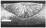
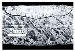 | ||
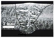
| TIG weld bead | ||
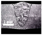
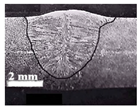
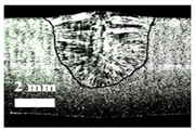
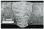 |  |  |
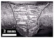
| ATIG weld with SiO2 oxide | ATIG weld with TiO2 oxide | ATIG weld with Fe2O3 oxide |
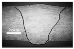
 | 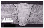 |  |
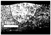
| ATIG weld with Cr2O3 oxide | ATIG weld with ZnO oxide | ATIG weld with Mn2O3 oxide |
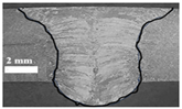 |  |  |
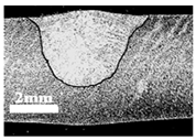
| ATIG weld with V2O5 oxide | ATIG weld with MoO3 oxide | ATIG weld with SrO oxide |
 |  |  |
| ATIG weld with ZrO2 oxide | ATIG weld with CaO oxide | ATIG weld with MgO oxide |
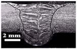
 |  |  |
| ATIG with Cr2O3, I = 150 A | ATIG with Cr2O3, I = 180 A | ATIG with Cr2O3, I = 200 A |
 |  |  |
| ATIG with Fe2O3, I = 150 A | ATIG with Fe2O3, I = 180 A | ATIG with Fe2O3, I = 200 A |
 |  |  |
| ATIG with ZnO, I = 150 A | ATIG with ZnO, I = 180 A | ATIG with ZnO, I = 200 A |
| X1 | X2 | X3 | X4 | X5 | X6 | X7 | X8 | X9 | I | D | R | |
|---|---|---|---|---|---|---|---|---|---|---|---|---|
| Mean | 838.9462 | 1876.7 | 2631.1 | 754.3846 | 445.3846 | 11.0401 | 984.3077 | 1283.4 | 724.8462 | 162.5 | 5.4653 | 0.6858 |
| Median | 824 | 1935 | 2850 | 670 | 400 | 11.1254 | 926 | 1400 | 648 | 165 | 4.51 | 0.5603 |
| Std.Dev | 301.2106 | 711.8393 | 918.4438 | 428.4565 | 236.3402 | 0.7578 | 711.8393 | 765.8080 | 395.7872 | 30.6066 | 2.3440 | 0.3215 |
| Range | 1200.6 | 2156 | 3220 | 1445 | 730 | 2.6642 | 2156 | 2555 | 1286 | 80 | 7.9642 | 1.1610 |
| Case of the Depth (D) | |||||||||
|---|---|---|---|---|---|---|---|---|---|
| Model | Training Data | Validation Data | All Data | ||||||
| R2 | MAPE (%) | RMSE (mm) | R2 | MAPE (%) | RMSE (mm) | R2 | MAPE (%) | RMSE (mm) | |
| Linear | 0.8037 | 17.7451 | 0.9826 | 0.7891 | 14.2530 | 1.0284 | 0.8166 | 16.8721 | 0.9943 |
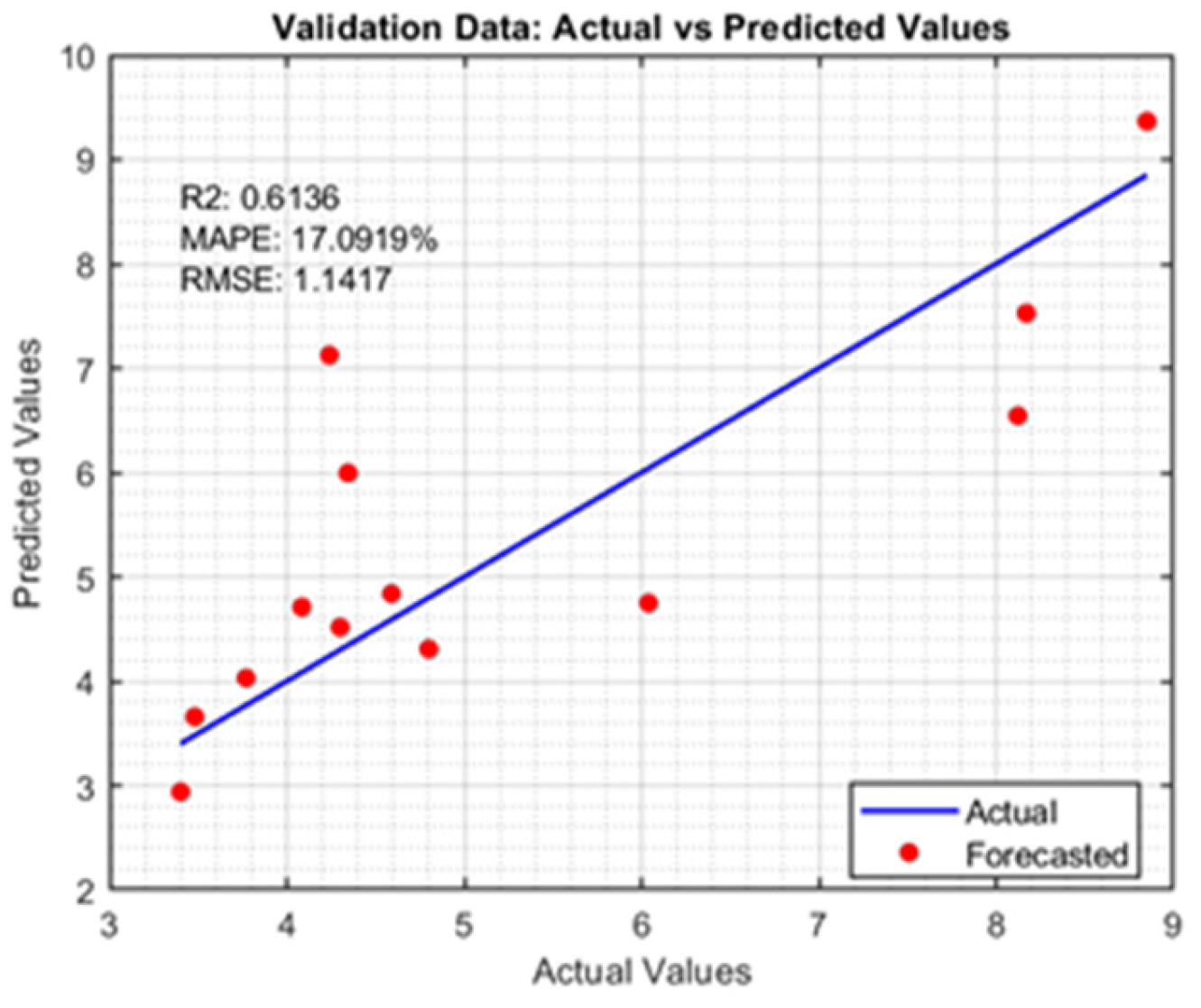
| Exponential | 0.8657 | 16.9677 | 0.9006 | 0.6136 | 17.0919 | 1.1417 | 0.8266 | 16.9988 | 0.9665 |
| Exponential model coefficients | a2 = −0.4027, b2 = −4.5012, a3 = 1.8803, b3 = 4.6587, a4 = 1.0334, b4 = −1.3178, a7 = −4.5852, b7 = −0.6760, a9 = −0.6875, b9 = 0.3861, aI = −0.1805, bI = −0.5464, c = −3.0939 | ||||||||
| Case of the Aspect Ratio (R) | |||||||||
|---|---|---|---|---|---|---|---|---|---|
| Model | Training Data | Validation Data | All Data | ||||||
| R2 | MAPE (%) | RMSE (mm) | R2 | MAPE (%) | RMSE (mm) | R2 | MAPE (%) | RMSE (mm) | |
| Linear | 0.6721 | 23.7241 | 0.1772 | 0.5789 | 26.0197 | 0.2206 | 0.6476 | 24.2980 | 0.1890 |
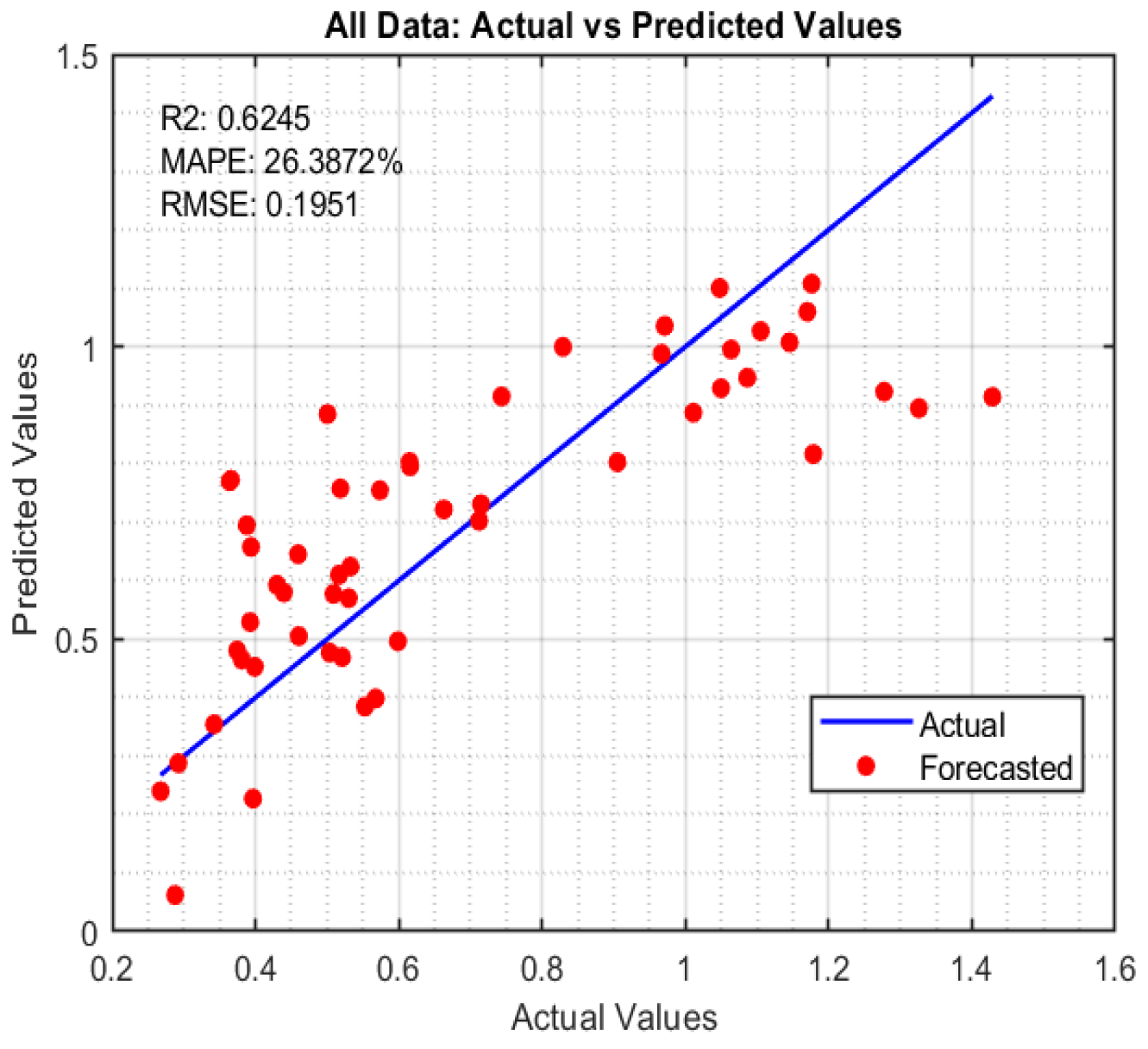
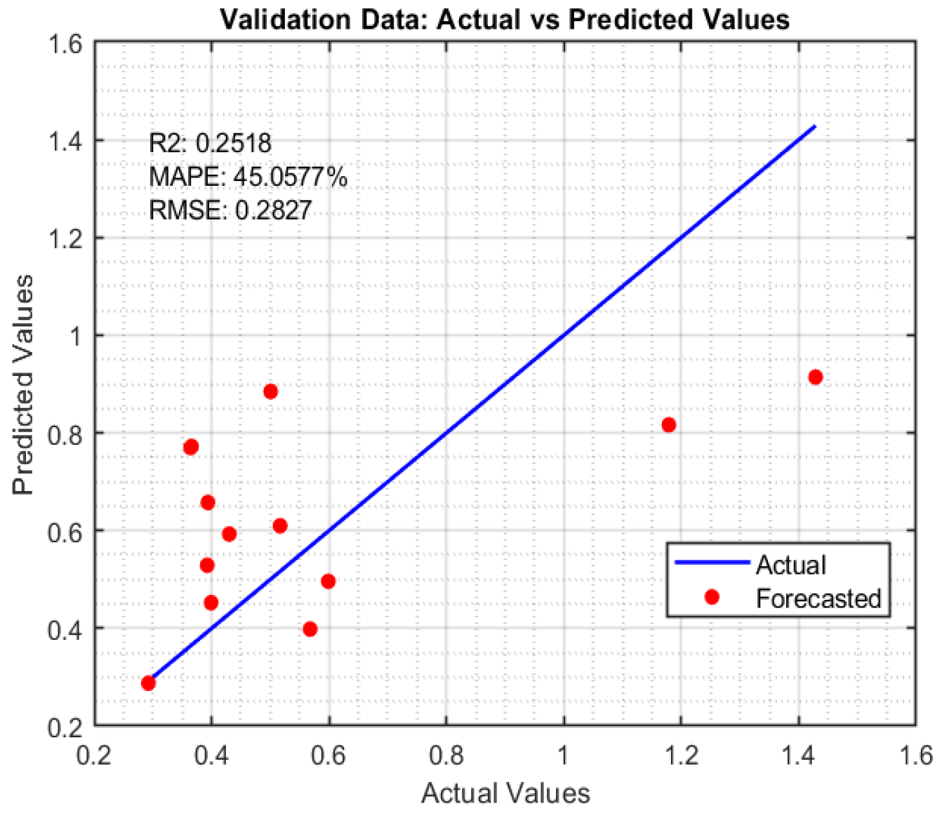
| Exponential | 0.7428 | 20.1637 | 0.1553 | 0.2518 | 45.0577 | 0.2827 | 0.6245 | 26.3872 | 0.1951 |
| Exponential model coefficients | a2 = −0.8827, b2 = 4.3788, a3 = −1.7359, b3 = −0.5112, a4 = −0.4685, b4 = −1.4612, a7 = −4.0338, b7 = −0.3008, a9 = −0.4195, b9 = −4.9970, aI = −2.1052, bI = −0.4201, c = −0.1825 | ||||||||
| Industry Field | Dtarget (mm) | X2/X2opt | X3/X3opt | X4/X4opt | X7/X7opt | X9/X9opt | I/Iopt | Dopt | Error |
|---|---|---|---|---|---|---|---|---|---|
| Power plant | 10 | 0.1260 941.6298 | 0.4906 2659.8 | 0.8988 1438.7 | 0.0180 73.8 | 0.3957 599 | 0.3334 146.6 (150) | 10.003 | 0.003 |
| Automotive | 5 | 0.6773 2130.3 | 0.3820 2309.9 | 0.6771 1118.4 | 0.9439 2070.0 | 0.7593 1066.5 | 0.9075 192.6 (190) | 5.012 | 0.012 |
| Construction | 12 | 0.8855 2579.0 | 0.4854 2643.1 | 0.0278 180.1 | 0.7159 1578.5 | 0.8138 1136.5 | 0.0579 124.6 (120) | 11.98 | 0.02 |
| Design Parameters | Envelope Lower Limit | Envelope Upper Limit | |
|---|---|---|---|
| Dtarget [mm] | 1.5 | 12 | |
| X2 | Oxide melting point (TM) [°C] | 670 | 2826 |
| X3 | Oxide boiling point (TB) [°C] | 2134 | 2701 |
| X4 | Oxide boiling and melting points difference (TB–TM) [°C] | 140 | 1585 |
| X7 | |Base metal boiling point–Oxide melting point (TM)|[°C] | 35 | 2191 |
| X9 | |Oxide melting point flux (Tm)–Base metal melting point| [°C] | 90 | 1376 |
| Welding current [A] | 120 | 200 | |
Disclaimer/Publisher’s Note: The statements, opinions and data contained in all publications are solely those of the individual author(s) and contributor(s) and not of MDPI and/or the editor(s). MDPI and/or the editor(s) disclaim responsibility for any injury to people or property resulting from any ideas, methods, instructions or products referred to in the content. |
© 2025 by the authors. Licensee MDPI, Basel, Switzerland. This article is an open access article distributed under the terms and conditions of the Creative Commons Attribution (CC BY) license (https://creativecommons.org/licenses/by/4.0/).
Share and Cite
Touileb, K.; Boubaker, S. Optimization of ATIG Weld Based on a Swarm Intelligence Approach: Application to the Design of Welding in Selected Manufacturing Processes. Crystals 2025, 15, 523. https://doi.org/10.3390/cryst15060523
Touileb K, Boubaker S. Optimization of ATIG Weld Based on a Swarm Intelligence Approach: Application to the Design of Welding in Selected Manufacturing Processes. Crystals. 2025; 15(6):523. https://doi.org/10.3390/cryst15060523
Chicago/Turabian StyleTouileb, Kamel, and Sahbi Boubaker. 2025. "Optimization of ATIG Weld Based on a Swarm Intelligence Approach: Application to the Design of Welding in Selected Manufacturing Processes" Crystals 15, no. 6: 523. https://doi.org/10.3390/cryst15060523
APA StyleTouileb, K., & Boubaker, S. (2025). Optimization of ATIG Weld Based on a Swarm Intelligence Approach: Application to the Design of Welding in Selected Manufacturing Processes. Crystals, 15(6), 523. https://doi.org/10.3390/cryst15060523