Article

Prediction of Temperature Factors in Proteins: Effect of Data Pre-Processing and Experimental Conditions

by
Jure Pražnikar
1,2
1
Faculty of Mathematics, Natural Sciences and Information Technologies, University of Primorska, Glagoljaška 8, 6000 Koper, Slovenia
2
Department of Biochemistry, Molecular and Structural Biology, Institute Jožef Stefan, Jamova 39, 1000 Ljubljana, Slovenia
Crystals 2025, 15(5), 455; https://doi.org/10.3390/cryst15050455
Submission received: 21 April 2025 / Revised: 8 May 2025 / Accepted: 9 May 2025 / Published: 12 May 2025
(This article belongs to the Section Macromolecular Crystals)

Abstract

:
The B-factor or temperature factor is one of the most important parameters in addition to the atomic coordinates, and which is refined during the determination of the protein structure and stored in the Protein Data Bank. It reflects the uncertainty of the atomic positions and is closely linked to atomic flexibility. By using graphlet degree vectors as feature descriptors in a linear model—together with appropriate data transformation and consideration of various experimental factors—the model provides better prediction results. For example, the inclusion of crystal contacts in the linear model significantly improves the prediction accuracy. Since the distributions of the B-factors typically follow an inverse gamma distribution, applying a logarithmic transformation further improves the performance of the model. It has also been shown that large ligands, such as those found in protein–DNA complexes, have a significant impact on the quality of the prediction. A linear model based on graphlet degree vectors proves to be effective not only for the prediction of B-factors and the validation of deposited protein structures but also for the qualitative estimation of root-mean-square fluctuations derived from molecular dynamics.

1. Introduction

Proteins play an important role in practically every cellular process. Their functions, which range from catalyzing biochemical reactions to mediating cell-to-cell communication, are closely linked to their three-dimensional structures. Therefore, understanding protein structure is fundamental to expanding our knowledge of complex biological systems. An important aspect of protein structure is its flexibility. Proteins are not static entities but exhibit a certain degree of conformational plasticity that is crucial for their biological functions. Atomic displacement parameter, also known as the B-factor or temperature factor [1,2], provide valuable insights into the inherent flexibility of protein structure [3,4]. Derived from X-ray crystallography, this parameter quantifies the average displacement of individual atoms within a protein. A higher B-factor indicates greater movement of the atoms, suggesting regions of increased flexibility. Accurate prediction of B-factors is therefore of paramount importance as it allows researchers to study protein dynamics and gain an understanding of protein function.
A number of methods have been introduced to predict the B-factor of proteins based on packing density [5], graph theory [6,7,8], amino acid sequence [9,10,11,12], variations in local structural composition [13], elastic networks of Cα atoms [14], and deep learning algorithms [15,16]. Weiss (2007) [17] pioneered the development of a linear model based on the parameters of close atomic contacts to predict B-factors. This original model was later improved by incorporating more sophisticated features, such as information about the complex network of interactions within the protein structure. This complex network can be described using graphlet orbits, a concept introduced by Pržulj (2007) [18]. Graphlets are small, induced subgraphs that allow us to describe the local connectivity patterns around the nodes in the graph. Including graphlet orbits as a feature in a multiple linear regression model has been shown to improve the accuracy of predicting the B-factor [19]. In addition to the linear models, the thermal fluctuations were evaluated using the Kirchhoff matrix, which is also known as the Laplacian matrix in spectral graph theory. The inverse of the Kirchhoff matrix, whose diagonal elements reflect the thermal motion of the atoms, proved to be suitable for estimating the B-factors of the Cα atoms [20,21,22]. However, there are still some important challenges that need to be addressed to improve B-factor prediction. These challenges can be broadly divided into two categories: (i) data transformation (or pre-processing) and (ii) experimental conditions.
Data pre-processing or data transformation is the crucial first step in creating predictive models, as using raw data can affect the performance of the algorithms. For example, the distribution of B-factors in the protein model is not normal but rather skewed towards large B-factors. It has been shown that the distribution of B-factors follows an inverse gamma distribution [23,24].
Normalization or scaling is also required to compare B-factors between different proteins [13,25,26,27]. Note that B-factors vary not only due to actual atomic mobility, but also due to conditions related to computational methods (refinement) and X-ray diffraction. There are different but fairly standardized protocols for scaling protein B-factors before performing a qualitative and quantitative comparison. The two most common approaches are Z-score normalization and rescaling of B-factors in the range from 0 to 100 [28,29]. However, a unit cell can also contain multiple chains (e.g., multimeric proteins), and these chains can have significantly different B-factors. For example, the average B-factor of one monomer in a dimer may be 12 Å2, while the other monomer has an average value of 33 Å2 [30]. Therefore, scaling of B-factors is required before a comparison can be made between monomers in multimeric proteins. This is particularly important when analyzing protein structures containing multiple chains (multimers) or mobile domains where bimodal or multimodal B-factor distributions can be observed [23,24]. Therefore, B-factor scaling is crucial when performing comparisons both within and between proteins.
In addition to the data transformation, the unique properties of X-ray crystallography must also be taken into account when preparing the data for the creation of the model. The proteins in the crystal are densely packed, resulting in numerous crystal contacts. Due to the crystal symmetry, the molecule in the asymmetric unit is surrounded by 7–10 molecules on average [31]. Hinsen (2008) [32] investigated the effects of close crystal contacts on atomic fluctuations using egg white lysozyme. The study demonstrated that crystal packing interactions can significantly influence the magnitude of atomic fluctuations. Although several studies have considered crystal contacts, they have not systematically evaluated the performance of models with and without the inclusion of crystal packing information.
X-ray crystallography is a powerful technique that is used not only to determine protein structure but also, and very importantly, to study the detailed spatial arrangement and interactions between proteins and their ligands. However, a comprehensive analysis of the effects of ligands on the accuracy of B-factor prediction in protein–ligand complexes is still largely unexplored. Kondrashov et al. (2006) [33] found a slight improvement in accuracy when ligands were included in their chemical network model to estimate Cα-atom flexibility. On the other hand, the linear model developed by Weiss (2007) [17] and the multiple linear model based on the graphlet degree vector [19] do not consider ligand atoms. Similarly, the influence of ligands and heteroatoms on B-factor prediction is not discussed in the work of Bramer and Wei (2018) and Pandey et al. (2023) [15,16], who used more advanced machine learning techniques to predict B-factors.
In order to improve data pre-processing and thereby increase the accuracy of the multiple linear model, this study aims to analyze how data transformation and the unique properties of X-ray crystallography affect the prediction and interpretation of B-factors in protein structures. This research therefore evaluates the impact of logarithmic transformation of B-factors on prediction accuracy and extends the knowledge of how appropriate scaling (or normalization) of B-factors improves their interpretation. In addition, the influence of large ligands and crystal contacts on the prediction of B-factors is evaluated. All these advances can significantly contribute to the accuracy of predicted B-factors and thus improve the interpretation of protein flexibility. Finally, the usefulness of a multiple linear model for the qualitative estimation of atomic positional fluctuations calculated by molecular dynamics is demonstrated.

2. Methods

2.1. Graphlet Degree Vector and Multiple Linear Model

Graphlets are small, connected, and non-isomorphic induced subgraphs. Figure 1A illustrates all eight graphlets up to a size of four nodes. These graphlets serve as building blocks to describe the local neighborhood of a node within a larger graph. The graphlet degree vector (GDV) of a node counts how often the node “touches” each type of graphlet. The GDV can also be thought of as a feature vector, where each element corresponds to a specific graphlet type and its value represents the frequency with which the node participates in that graphlet. Therefore, the GDV effectively captures the local connectivity pattern of a particular node.
The graphlets shown in Figure 1A contain fifteen topologically different nodes, labeled 0 to 14. Nodes with the same topological neighborhood belong to the same orbit. Since there are fifteen different node orbits within graphlets with up to four nodes, the GDV has a length of fifteen. For example, node I in the graph shown in Figure 1B has three edges, which are reflected in the first element of its GDV (Figure 1C). In addition, node I is involved in one instance of the orbit O3 (triangle). In other words, the first column of the GDV matrix (Figure 1C) represents the number of edges for each node, while column four, which corresponds to orbit O3, describes the frequency of triangle participation. Orbit O3 can be described as follows: Node I has neighboring nodes (H and J), and these two neighboring nodes are also connected to each other. The GDV is calculated for each node in the large graph and serves as an independent variable in a multiple linear model, which is written as follows:
B n = b 0 + β 0 O n , 0 + β 1 O n , 1 + + β k O n , k
where Bn is the dependent variable, n =1, 2, …, N; N is the number of nodes (atoms); b0 is the intercept; On,k, k = 0, 1, 2, …, 14, are explanatory variables; and βk, are the coefficients of the regression vector. A matrix of size Nx15 (where N is the number of atoms) was created for each protein. This matrix was then normalized (column-wise) before being used to create the linear model. A 10-fold cross-validation procedure was used to validate the GDV-based linear model. In each fold, the model was trained on 90% of the data (1760 proteins) and used to predict the B-factors for the remaining 10% (196 proteins).

2.2. Data Pre-Processing of Dependent Variable

Six data sets with different pre-processing approaches were created. The techniques used to pre-process the data are divided into four categories: (i) crystal or symmetric contacts, (ii) log transformation, (iii) scaling or normalization, and (iv) inclusion of ligand atoms (Table 1). Three distance thresholds were used when considering crystal contacts: 0 Å, 7.5 Å and 15 Å. Adjacent copies were generated from the biological unit of the protein using crystallographic symmetry operations. Symmetry-related residues were included in the construction of the larger graph if the distance between the Cβ atoms of the reference and copy molecules was less than the specified threshold. In data sets 4, 5 and 6, the dependent variable was log transformed before scaling. For each protein, the dependent variable (B-factor) was scaled using the Z-score method, resulting in data with a mean of zero and a standard deviation of one. Scaling was applied either to the entire biological unit or independently to individual chains within the biounit (per-chain scaling). Per-chain scaling was performed on proteins that contained more than one chain in the biological unit and the following three criteria were met: (i) the ratio between the length of the longer chain and the shorter chain is less than 1.5, (ii) the ratio between the mean B-factors of the chains is greater than 1.25, and (iii) the difference between the mean B-factors of the chains is greater than 5 A2. These criteria were applied when the protein model has up to three different chains. For the entries with multiple chains (four or more), per-chain scaling was not applied. This criterion was used to select cases where the mean B-factor between the chains was significantly different and, at the same time, the length between the chains was of the same order of magnitude. The per-chain scaling was not applied if the biological unit contained, for example, the protein and a short peptide.
Ligand atoms were considered close contacts of protein atoms and included in the larger graph if the size of the ligand (total number of atoms) was at least 10% of the size of the protein and if at least 10% of the amino acids of the protein had close contacts with the ligand. A close contact was defined as a distance of 5 Å or less between the Cβ atom of a protein and any ligand atom. This approach focused on cases where the ligand was of comparable size to the protein and where a significant proportion (greater than 10%) of the protein’s atoms were in close proximity to the ligand.

2.3. Data Set and Software

This study uses a dataset of 1956 proteins that was originally used by Pražnikar (2023) [19] for the creation and validation of the linear GDV model. Therefore, a brief overview of the protein selection process is given here. The Protein Sequence Culling Server [34] was used to generate a list of PDB IDs based on the following criteria: sequence identity no greater than 40%, X-ray resolution between 1.6 Å and 2.6 Å, crystallographic R-value ≤ 0.25, and protein size between 50 and 500 residues. This initial list was further filtered to exclude: (1) assemblies with more than 10,000 atoms; (2) proteins with missing B-factors; (3) assemblies with B-factors above 200; and (4) assemblies with a B-factor standard deviation below 0.1. The re-refined and rebuilt protein structures were retrieved from the PDB-REDO database [35,36]. PDB-REDO applies modern refinement protocols (consistent procedures) to existing PDB entries, often resulting in models with higher accuracy and better fit to the experimental data. The pipeline also includes rebuilding steps to correct common modeling errors, such as incorrect side chain conformations or peptide plane orientations. The PDB-REDO database is particularly suitable for large-scale analyses and comparisons as it applies a consistent and automated refinement workflow that reduces variability caused by different refinement strategies, specific software algorithms, and user-defined settings.
Each 3D protein model was converted into a graph-based representation. First, all pairwise inter-atomic distances within the protein structure were calculated. Then, an adjacency matrix encoding the atomic connectivity was created: an edge was created between two atoms if their distance was less than 7.0 Å. This adjacency matrix defined the graph that was subsequently used to calculate GDV for each atom.
The R package (version 4.2.2) [37] was used for data analysis with the following packages: orca (version 1.1-3) [38,39], netdist (version 0.4.9100) [40], bio3d (version 2.4-5) [41], igraph (version 2.1.2) [42], caret(version 7.0-1) [43], cry (version 0.5.1), and pdsit (version 1.2.1). R scripts with an example can be found at https://github.com/jure-praznikar/B-factor-prediction.

2.4. Molecular Dynamic

Molecular dynamics (MDs) simulations were performed to investigate the dynamic behavior (root-mean-square fluctuations) of the proteins. The initial structures, identified by the PDBid’s: 2qmt, 1ubq, and 1pgb, have a crystallographic resolution of 1.05 Å, 1.80 Å, and 1.92 Å, respectively. All simulations were performed using the GROMACS (version 2024.4) package and the CHARMM36 (July 2022) force field [44,45,46]. Each protein was solvated in a cubic box of TIP3P water molecules, keeping a minimum distance of 1.0 nm between the protein and the edges of the box. To mimic physiological conditions, sodium (Na+) and chloride (Cl) ions were added to neutralize the system and achieve a salt concentration of 0.15 M. Prior to MDs simulations, energy minimization was performed using the steepest descent algorithm until the maximum force was reduced to below 1000 kJ/mol/nm2, effectively removing steric clashes and unfavorable contacts. The system was then equilibrated in two steps. First, a 200 ps simulation was performed in a canonical ensemble (NVT) using the Nosé-Hoover thermostat (1 ps coupling) to maintain a constant temperature of 300 K. A 1 ns simulation was then performed in an isothermal–isobaric thermodynamic ensemble (NPT) using the Nosé-Hoover thermostat (300 K, 1 ps coupling) and the Parrinello-Rahman barostat (1.0 bar, 5 ps coupling) to equilibrate pressure and density. The MDs production runs were performed in the NPT ensemble at 300 K for 100 ns, with a time step of 2 fs and using periodic 3D boundary conditions. The LINCS algorithm was used to constrain all covalent bonds involving hydrogen atoms. Electrostatic interactions were calculated using the Particle Mesh Ewald summation method and van der Waals interactions were truncated at 1.2 nm. Snapshots of the simulation trajectory were saved every 10 ps. Root-mean-square fluctuations (RMSFs), a commonly used measure of conformational variability, were calculated for the main chain atoms (N, Cα, C, O) using GROMACS software.

3. Results and Discussion

3.1. The Improvement of Linear GDV Model

The linear GDV model was built on the data set of 1957 proteins but using different pre-processing approaches that include symmetry contact information, log transformation of B-factors, per-chain scaling of B-factors, and consideration of large ligands. The lowest correlation between deposited and predicted B-factors was achieved when no crystal contact (dataset 1) was used (
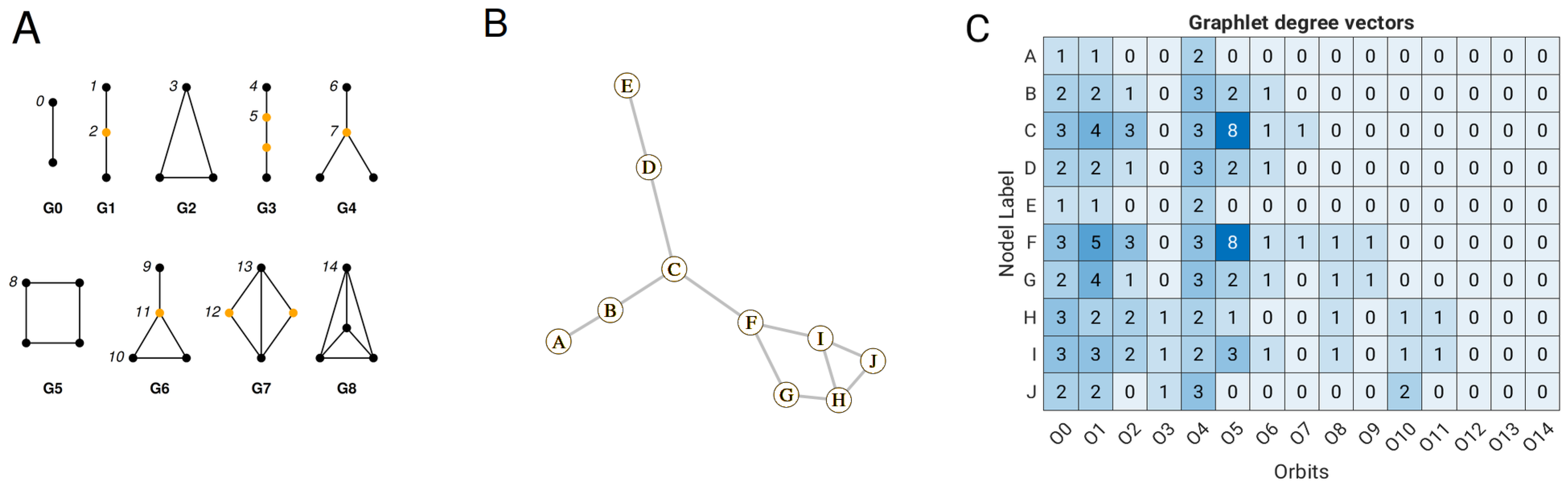
Figure 2). This suggests that the introduction of packing atom information improves the accuracy of B-factor prediction. It is interesting to see that the performance of the linear GDV model increased slightly when the cutoff distance for close crystal contact was extended from 7.5 Å to 15 Å. This seems contradictory since the cutoff distance for the construction of the graph was 7 Å, and the longer cutoff distance (extension from 7.5 Å to 15 Å) should not have any effect at first sight. The explanation for this is as follows: Increasing the cutoff distance has no effect on the orbit O0, which is one edge deep and is the first feature of GDV. But it can affect, for example, orbits O5 and O10 (Figure 1A), which contain information about deep contacts (up to 3 edges). Furthermore, the log transformation improved the average correlation from 0.75 (dataset 3) to 0.77 (dataset 4). This transformation helps to achieve a more normal distribution of the B-factors, which typically follow an inverse gamma distribution, and also attenuates the influence of outliers, thus improving the performance of the linear GDV model. Figure S1 shows the coefficients of the linear GDV model, and it can be seen that the coefficients of the first three models where the cutoff distance of close contacts was increased from 0 Å to 7.5 Å and finally to 15 Å, are different, while for the linear GDV models where the log transformation, per-chain scaling, and ligand contacts were applied (dataset 4, 5, and 6), the coefficients of the linear model are more or less the same. In other words, the inclusion of crystal contacts changes the linear model directly, whereas the log transformation, per-chain scaling, and ligand contacts do not. The source of improvement in the latter cases is therefore a better quality of the data, either due to the appropriate per-chain scaling or due to the inclusion of the ligand atoms as close contacts. The final model (dataset 6) achieves a correlation of 0.78. It is worth noting that a recent study [16] using a sequence-based deep learning model found a correlation of 0.8 for a dataset of 2442 proteins. Note that their analysis was limited to Cα atoms, whereas this study considers all protein atoms.
Anyway, we see that the per-chain scaling and the introduction of ligand atoms as close contacts do not lead to a significant improvement in the prediction of the whole dataset. The mean correlation value of log transformation (dataset 4), per-chain scaling, (dataset 5) and the introduction of ligand atoms as close contacts (dataset 6) is very similar (Figure 2). The reason for this is that the log transformation is used in all protein models, while the per-chain scaling and the consideration of ligand atoms as close contacts are not used for all entries in the dataset. The per-chain scaling and the introduction of ligand atoms as close contacts were only used in a limited number of cases, 77 and 142, respectively. However, we can detect two outliers with a very low correlation (0.2 and 0.3) in the log transformation case (dataset 4), but these two outliers no longer exist in the per-chain scaling case (dataset 5), and when ligand atoms were used as close contacts (dataset 6). However, a closer look at the box-plot shows that the shortest whisker defining the lower outliers can be observed when using dataset 6. This dataset includes the log transformation, the per-chain scaling and the inclusion of ligand atoms (Table 1).
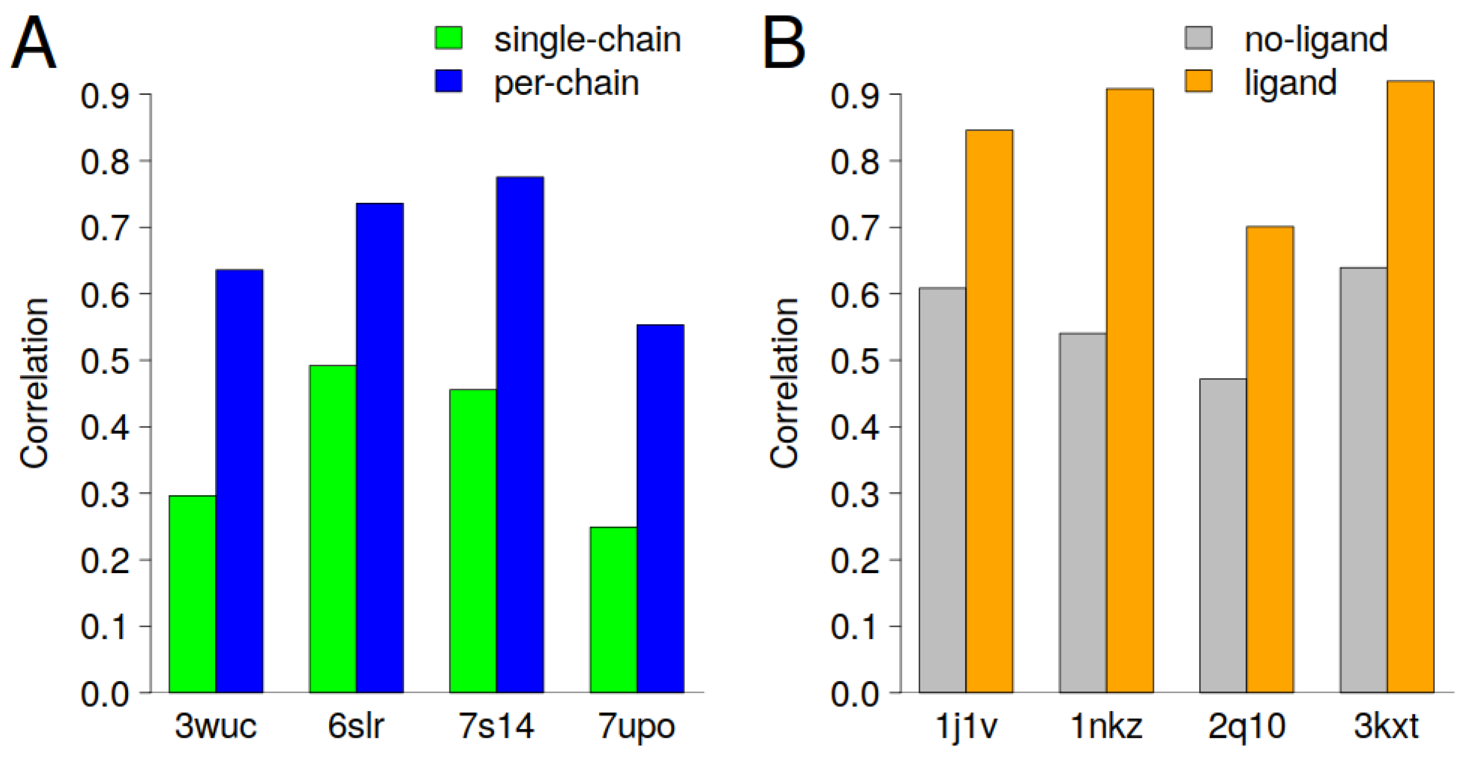
Figure 3 shows the cases with the largest improvements in correlation (>0.2) in the case of per-chain scaling and the introduction of ligand atoms as close contacts. It should be emphasized that the introduction of ligand atoms as close contacts and per-chain scaling is a case-dependent problem and that cryptographers should design and implement solutions that are specifically tailored to the unique characteristics of each case. For example, the protein could have a bimodal distribution of B-factors within a single chain, or a multimodal distribution that corresponds to translation–libration–screw groups rather than cryptographer-defined chain IDs. In addition, a statistical approach, e.g., Hartigan’s dip test for bimodality, can be used to decide whether the B-factors should be scaled according to defined groups. The next section discusses eight cases in which the prediction of the B-factor was significantly improved.

3.2. Case Studies—Per-Chain Scaling

The results presented in Figure 3A demonstrate that per-chain scaling can enhance the interpretation of the predicted B-factors. For all four cases presented, we can see an increase in correlation of about 0.3 when per-chain scaling was applied. It is clear that the largest improvement was observed for entries that are homomeric or heteromeric proteins (Figure S2A–D).
The biounit of PDBids: 3wuc, 6slr and 7s14 have two chains and the comparison of B-factors within each biounit shows that the mean B-factors are quite different (Figure 4A,D,G). The PDBid: 3wuc case, for example, chain A has a mean B-factor of 22A2, while chain B has a mean B-factor of 8A2. The two clusters corresponding to two chains can also be seen in the scatter plots in Figure 4B, while in Figure 4C, where the B-factors are per-chain scaled, no separate groups can be seen. A similar conclusion can also be drawn for PDBid’s: 6slr and 7s14, where no separate clusters and a higher correlation were observed when per-chain scaling was applied (Figure 4E,F,H,I).
More complex scenarios arise for proteins with three or more chains (Figure S2D). We can see that in the case of PDBid: 7upo, two chains, namely A and B, have similar mean B-factors, while chain C has significantly higher B-factors (Figure 4J). In this particular case, per-chain scaling improved from a rather low (0.25) to a medium (0.55) correlation (Figure 4K,L).
Scaling is usually obligatory when B-factors are compared between proteins. In this study, the results suggest that, in some cases, per-chain scaling is required when dealing with homomeric or heteromeric proteins containing subunits with significantly different B-factors within the same unit cell. A direct comparison of the deposited B-factors between chains A, B, and C of PDBid:7upo without normalization could falsely give the impression that all atoms in chain C are more flexible than those in chains A and B. Higher deposited B-factors of chain C are probably related to crystallization effects, e.g., packing and symmetry-related interactions.
It is worth noting that the per-chain scaling does not change the independent variables. This is because the features or independent variables are only based on coordinates, parameters used in the construction of the graph, and the cutoff distance for the formation of node edges, while the per-chain scaling is related to the log transformation of the dependent variable.

3.3. Case Studies—Ligand Atoms as Close Contacts

Similar to the improvements observed in the implementation of per-chain scaling, the inclusion of ligand information in the construction of the graphs, which consequently affects the GDVs (features), can significantly improve the prediction of the B-factors in certain cases (see Figure 3B). It is noteworthy that three of the four cases in which the correlation was significantly improved involved protein–DNA complexes (Figure S3A–C). In these complexes, about 30% of the amino acids are in close contact with the ligand.
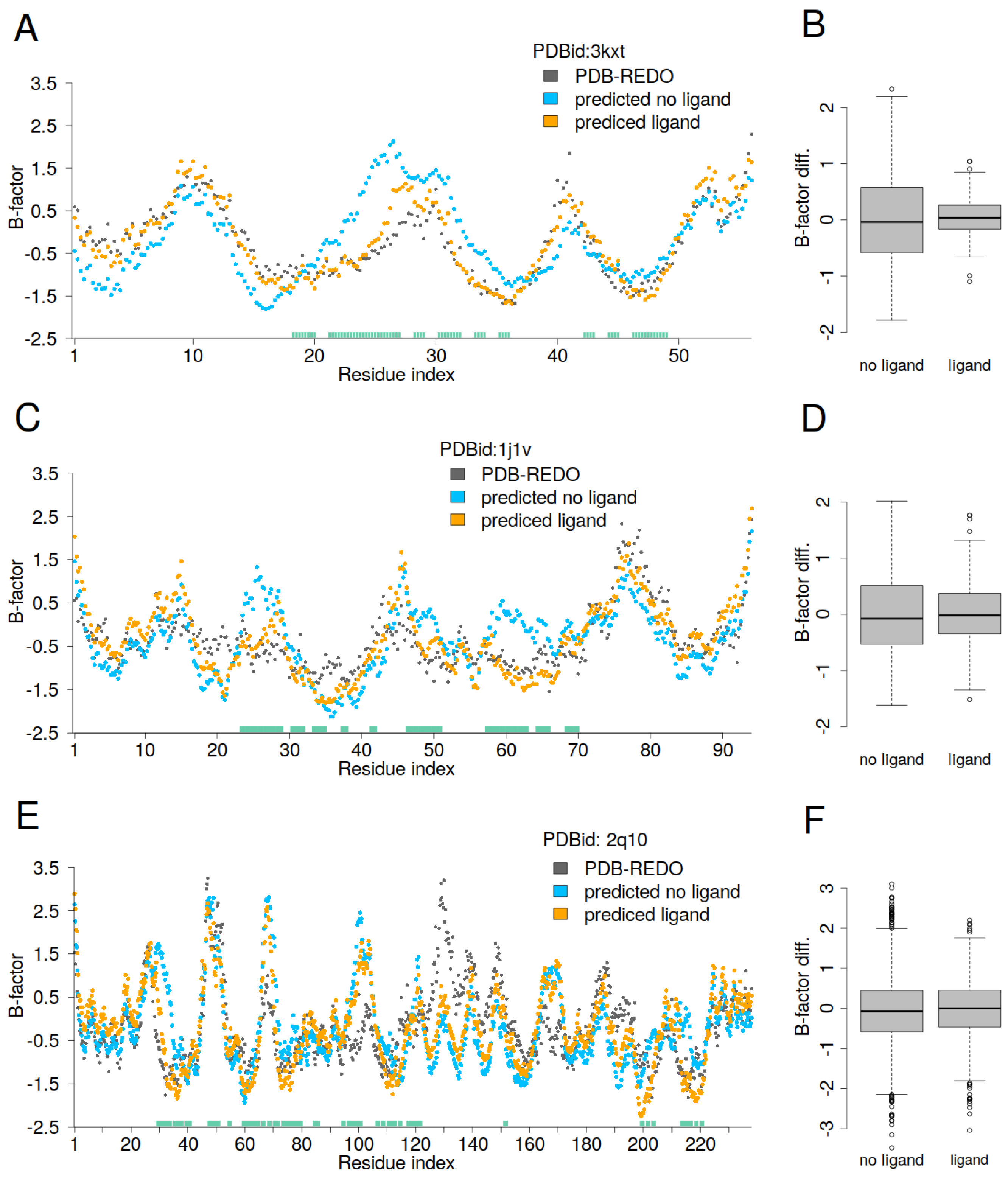
For the protein PDBid: 3kxt, residues from 20 to 35 show significantly higher predicted B-factors when the ligand is not present (Figure 5A). For the protein PDBid: 1j1v, residues 25, 48, and 60, as well as the neighboring residues, also exhibit higher predicted B-factors when the ligand is excluded from the calculation (Figure 5C). For the protein PDBid: 2q10, the clearest differences between the predicted and PDB-REDO B-factors occur around residue 30 and residues 200–220 (Figure 5E). These regions correspond to the close contacts with the DNA. Remarkably, in addition to the overestimated B-factors, we also observe underestimations (lower B-factors) in regions where there are no close contacts between protein and DNA. The boxplots (Figure 5B,D,F) show the difference between the PDB-REDO and predicted B-factors, and we can see that the linear GDV model both overestimates and underestimates the B-factors, with greater scatter when the ligand is not taken into account. While one might expect discrepancies primarily in regions of close contact between protein and ligand, a more comprehensive analysis of the entire protein, not just the contact region, is required. Ligand inclusion or exclusion alters the topology of the protein–ligand complex by redefining the boundaries between inner and outer residues. Residues that were previously classified as surface-exposed can become core residues as a result of ligand inclusion. Conversely, some core protein residues are less deeply buried within the protein–ligand complex than in the protein alone. This transition changes the interpretation of mobile and rigid residues. In general, residues that appear to move from core positions to more exposed positions within the protein–ligand complex exhibit increased relative flexibility. Conversely, residues at the protein–ligand interface tend to show lower relative flexibility.
The fourth example (PDBid: 1nkz) is the integral membrane light-harvesting complex II (LH2) of Rhodobacter sphaeroides strain 10050. This model contains bacteriochlorophylls and rhodopin glucoside as non-protein atoms (Figure S3D). Remarkably, almost all amino acids exhibit close contact to these heteroatoms, and the distribution of predicted B-factors differs significantly when comparing models with and without ligand atoms (Figure 6A). The correlation between PDB-REDO and the predicted B-factors increases from 0.54 to 0.91 when heteroatoms are also taken into account (Figure 3B). The exclusion of heteroatoms from the model falsely suggests that the central region of the protein, which corresponds to the membrane-embedded region, is very flexible. This misinterpretation arises because the model incorrectly predicts high B-factors in the protein region that interacts with the membrane. Figure 6B illustrates a larger discrepancy, namely the underestimation and overestimation of B-factors when heteroatoms are excluded in the construction of the graph.
These cases demonstrated that not only the contacts of the crystal packing but also the presence of large ligands, especially when their molecular weight is comparable to that of the protein, can significantly affect the prediction of B-factors in the crystal structure.

3.4. Qualitative Estimation of the Atom Fluctuations

Although experimental B-factors provide valuable insights into protein flexibility and function, it is important to recognize their inherent limitations. B-factors are affected by experimental errors, data resolution, misplaced atoms in the protein model, radiation damage and crystal packing contacts. The latter can cause the determined B-factors to be artificially low, especially for outer residues, suggesting that certain regions of the protein structure can be more rigid than reasonably expected in the aqueous environment. In addition to the crystallographic B-factors, root–mean–square fluctuations calculated by molecular dynamics simulations can also be used as a powerful method to study protein flexibility. However, we should be aware that molecular dynamics also has its drawbacks. For example, it is strongly dependent on force fields, i.e., empirically parameterized equations to calculate the potential energy of a system of atoms. Despite some differences between the experimentally determined B-factors and the root–mean–square fluctuations of molecular dynamics (MD-RMSF), the conclusions on protein flexibility are generally consistent, although not identical.
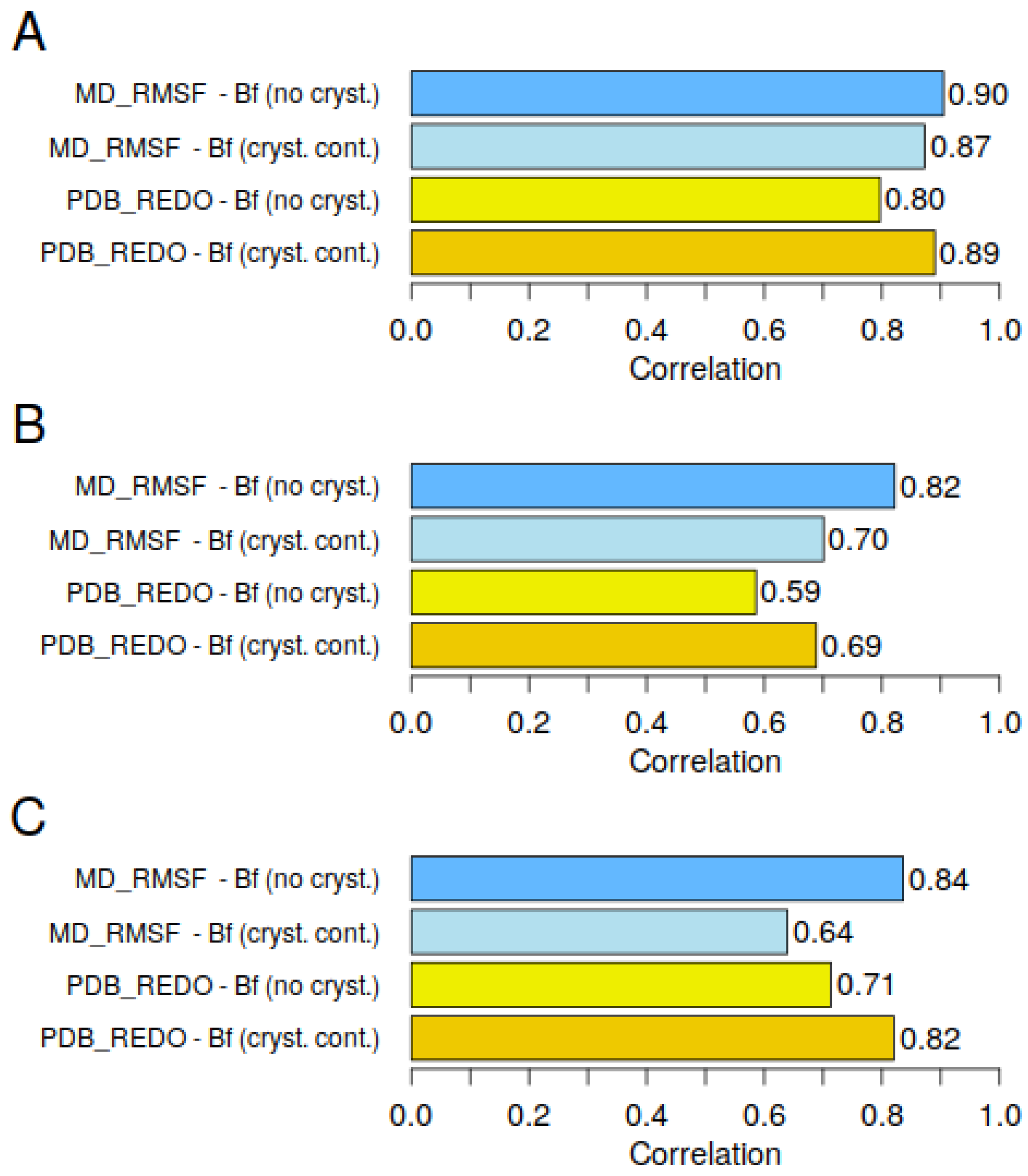
Figure 7 shows the correlation between the experimental B-factors, the MD-RMSF. and the predicted B-factors. Two approaches were used to predict the B-factors: with and without crystal contacts. Again, it was confirmed that the crystal packing information improves the prediction of the crystallographic B-factors. Interestingly, however, the opposite effect is observed when the predicted B-factors are compared with the MD-RMSF. The exclusion of close crystal contact improves the correlation between the predicted B-factors and the MD-RMSF. The linear GDV model provides accurate predictions for both the B-factors and the MD-RMSF and consistently achieves high correlations—greater than 0.69 in the cases presented—when symmetry packing interactions are adequately accounted for.
Therefore, the GDV model can be used as a validation tool for crystallographic B-factors and as a first approximation to the MD-RMSF. Moreover, the difference between these two options (with and without close crystal contacts) gives us an insight into the influence of crystal packing on the possible conformational changes of the protein induced by crystal packing. It is important to note that the training dataset for the linear GDV model presented in this study is based solely on crystallographic B-factors. Consequently, its main function is still to predict crystallographic B-factors and evaluate the quality of the underlying PDB structures. However, this example shows that simply switching the consideration of crystal contacts on and off can provide valuable qualitative insights into the potential influence of crystal packing on the crystallized protein.

4. Conclusions

In this study, the influence of data transformation and various experimental factors on the prediction of protein B-factors was analyzed. The analysis reveals a relationship between the inclusion of ligand atoms and the prediction of B-factors. However, a limitation of the presented approach is the focus on relatively large ligands and the use of arbitrarily defined selection criteria. It should be emphasized that the simple inclusion of mobile solvent molecules would increase the number of close contacts, which could lead to an overestimation of the rigidity of the outer atoms—a problem that also applies to small ligands. Therefore, further research is needed to find out which and how many heteroatoms significantly influence the flexibility of certain protein regions.
Crystal packing, an inherent consequence of X-ray crystallography, leads to specific intermolecular contacts due to crystal symmetry. These symmetry-related contacts are not present in experimental techniques such as nuclear magnetic resonance and cryo-electron microscopy. The investigation demonstrates that close-symmetry contacts significantly affect the accuracy of B-factor prediction and should be considered in the validation of crystallographic B-factors.
Furthermore, the study highlights that the linear GDV model performs worse when crystal contacts are excluded, but at the same time, the linear GDV model predicts the MD-RMSF better. Thus, while crystal contacts need to be considered when validating B-factors, the linear GDV model without crystal contacts is better suited to qualitatively estimate the flexibility of proteins in an aqueous environment.
Recent advances in AI-assisted prediction of protein structures, such as AlphaFold2 and Rosetta [47,48], have dramatically increased the number of available 3D protein structures. However, these algorithms predict atomic coordinates without providing B-factors, which are essential for studying protein flexibility and function. Indeed, the pLDDT score, which estimates the confidence in the AlphaFold2 predictions and is entered into the file in the column normally reserved for crystallographic B-factors, does not correlate with the experimental temperature B-factor [49].
A well-known limitation of X-ray-derived B-factors is that they contain experimental errors and primarily describe atomic displacement in a crystalline environment rather than in solution. A promising way to improve the linear GDV model to study protein flexibility could be the integration of molecular dynamics data. For example, ATLAS [50], a database of standardized molecular dynamics simulations, provides RMSF values for all protein atoms that can replace the crystallographic B-factors to develop a model for rapid, qualitative predictions of protein flexibility.

Supplementary Materials

The following supporting information can be downloaded at: https://www.mdpi.com/article/10.3390/cryst15050455/s1, Figure S1: The coefficients of the multiple linear regression for six different pre-processed datasets. Figure S2: Ribbon representation of the biological unit for (A) PDBid: 3wuc, (B) PDBid: 6slr, (C) PDBid: 7s14, and (D) PDBid: 7upo. Each chain within the biological unit is shown in a different color. Figure S3: Ribbon representation of the biological unit for (A) PDBid: 1j1v, (B) PDBid: 6slr, (C) PDBid: 2q10, and (D) PDBid: 1nkz. The protein is shown in ice-blue color, while the ligand is in green color.

Funding

This work was supported by Structural Biology grant P1-0048 and Infrastructure Programme grant I0-0035-2790 provided by the Slovenian Research Agency.

Data Availability Statement

The raw data supporting the conclusions of this article will be made available by the authors on request.

Conflicts of Interest

The authors declare no conflicts of interest.

References

  1. Dunitz, J.D.; Maverick, E.F.; Trueblood, K.N. Atomic motions in molecular crystals from diffraction measurements. Angew. Chem. Int. Ed. 1988, 27, 880–895. [Google Scholar] [CrossRef]
  2. Trueblood, K.N.; Bürgi, H.B.; Burzlaff, H.; Dunitz, J.D.; Gramaccioli, C.M.; Schulz, H.H.; Shmueli, U.; Abrahams, S.C. Atomic Displacement Parameter Nomenclature Report of a Subcommittee on Atomic Displacement Parameter Nomenclature. Acta Crystallogr. Sect. A Found. Crystallogr. 1996, 52, 770–781. [Google Scholar] [CrossRef]
  3. Karplus, P.A.; Schulz, G.E. Prediction of Chain Flexibility in Proteins. Naturwissenschaften 1985, 72, 212–213. [Google Scholar] [CrossRef]
  4. Schneider, B.; Gelly, J.C.; de Brevern, A.G.; Černý, J. Local Dynamics of Proteins and DNA Evaluated from Crystallographic B Factors. Acta Crystallogr. Sect. D Biol. Crystallogr. 2014, 70, 2413–2419. [Google Scholar] [CrossRef] [PubMed]
  5. Halle, B. Flexibility and Packing in Proteins. Proc. Natl. Acad. Sci. USA 2002, 99, 1274–1279. [Google Scholar] [CrossRef]
  6. Jacobs, D.J.; Rader, A.J.; Kuhn, L.A.; Thorpe, M.F. Protein Flexibility Predictions Using Graph Theory. Proteins Struct. Funct. Genet. 2001, 44, 150–165. [Google Scholar] [CrossRef]
  7. Gohlke, H.; Kuhn, L.A.; Case, D.A. Change in Protein Flexibility upon Complex Formation: Analysis of Ras-Raf Using Molecular Dynamics and a Molecular Framework Approach. Proteins Struct. Funct. Genet. 2004, 56, 322–337. [Google Scholar] [CrossRef]
  8. Yin, H.; Li, Y.-Z.; Li, M.-L. On the Relation Between Residue Flexibility and Residue Interactions in Proteins. Protein Pept. Lett. 2011, 18, 450–456. [Google Scholar] [CrossRef]
  9. Yuan, Z.; Bailey, T.L.; Teasdale, R.D. Prediction of Protein B-Factor Profiles. Proteins Struct. Funct. Genet. 2005, 58, 905–912. [Google Scholar] [CrossRef]
  10. Schlessinger, A.; Rost, B. Protein Flexibility and Rigidity Predicted from Sequence. Proteins Struct. Funct. Genet. 2005, 61, 115–126. [Google Scholar] [CrossRef]
  11. Schlessinger, A.; Yachdav, G.; Rost, B. PROFbval: Predict Flexible and Rigid Residues in Proteins. Bioinformatics 2006, 22, 891–893. [Google Scholar] [CrossRef] [PubMed]
  12. Pan, X.-Y.; Shen, H.-B. Robust Prediction of B-Factor Profile from Sequence Using Two-Stage SVR Based on Random Forest Feature Selection. Protein Pept. Lett. 2009, 16, 1447–1454. [Google Scholar] [CrossRef]
  13. Yang, J.; Wang, Y.; Zhang, Y. ResQ: An Approach to Unified Estimation of B-Factor and Residue-Specific Error in Protein Structure Prediction. J. Mol. Biol. 2016, 428, 693–701. [Google Scholar] [CrossRef]
  14. Kundu, S.; Melton, J.S.; Sorensen, D.C.; Phillips, G.N. Dynamics of Proteins in Crystals: Comparison of Experiment with Simple Models. Biophys. J. 2002, 83, 723–732. [Google Scholar] [CrossRef]
  15. Bramer, D.; Wei, G.-W.W. Blind Prediction of Protein B-Factor and Flexibility. J. Chem. Phys. 2018, 149, 134107. [Google Scholar] [CrossRef] [PubMed]
  16. Pandey, A.; Liu, E.; Graham, J.; Chen, W.; Keten, S. B-Factor Prediction in Proteins Using a Sequence-Based Deep Learning Model. Patterns 2023, 4, 100805. [Google Scholar] [CrossRef]
  17. Weiss, M.S. On the Interrelationship between Atomic Displacement Parameters (ADPs) and Coordinates in Protein Structures. Acta Crystallogr. Sect. D Biol. Crystallogr. 2007, 63, 1235–1242. [Google Scholar] [CrossRef]
  18. Pržulj, N. Biological Network Comparison Using Graphlet Degree Distribution. Bioinformatics 2007, 23, e177–e183. [Google Scholar] [CrossRef] [PubMed]
  19. Pražnikar, J. Using Graphlet Degree Vectors to Predict Atomic Displacement Parameters in Protein Structures. Acta Crystallogr. Sect. D Struct. Biol. 2023, 79, 1109–1119. [Google Scholar] [CrossRef]
  20. Tirion, M.M. Large Amplitude Elastic Motions in Proteins from a Single-Parameter, Atomic Analysis. Phys. Rev. Lett. 1996, 77, 1905–1908. [Google Scholar] [CrossRef]
  21. Bahar, I.; Atilgan, A.R.; Erman, B. Direct Evaluation of Thermal Fluctuations in Proteins Using a Single-Parameter Harmonic Potential. Fold. Des. 1997, 2, 173–181. [Google Scholar] [CrossRef] [PubMed]
  22. Haliloglu, T.; Bahar, I.; Erman, B. Gaussian Dynamics of Folded Proteins. Phys. Rev. Lett. 1997, 79, 3090–3093. [Google Scholar] [CrossRef]
  23. Masmaliyeva, R.C.; Murshudov, G.N. Analysis and Validation of Macromolecular b Values. Acta Crystallogr. Sect. D Struct. Biol. 2019, 75, 505–518. [Google Scholar] [CrossRef]
  24. Masmaliyeva, R.C.; Babai, K.H.; Murshudov, G.N. Local and Global Analysis of Macromolecular Atomic Displacement Parameters. Acta Crystallogr. Sect. D Struct. Biol. 2020, 76, 926–937. [Google Scholar] [CrossRef]
  25. Carugo, O.; Argos, P. Protein-Protein Crystal-Packing Contacts. Protein Sci. 1997, 6, 2261–2263. [Google Scholar] [CrossRef]
  26. Smith, D.K.; Radivojac, P.; Obradovic, Z.; Dunker, A.K.; Zhu, G. Improved Amino Acid Flexibility Parameters. Protein Sci. 2003, 12, 1060–1072. [Google Scholar] [CrossRef]
  27. Carugo, O. Atomic Displacement Parameters in Structural Biology. Amino Acids 2018, 50, 775–786. [Google Scholar] [CrossRef]
  28. Mlynek, G.; Djinović-Carugo, K.; Carugo, O. B-Factor Rescaling for Protein Crystal Structure Analyses. Crystals 2024, 14, 443. [Google Scholar] [CrossRef]
  29. Barthels, F.; Schirmeister, T.; Kersten, C. BANΔIT: B’-Factor Analysis for Drug Design and Structural Biology. Mol. Inform. 2021, 40, e2000144. [Google Scholar] [CrossRef]
  30. Williamson, A.; Rothweiler, U.; Leiros, H.-K.S. Enzyme–adenylate Structure of a Bacterial ATP-Dependent DNA Ligase with a Minimized DNA-Binding Surface. Acta Crystallogr. Sect. D 2014, 70, 3043–3056. [Google Scholar] [CrossRef]
  31. Carugo, O.; Djinović-Carugo, K. How Many Packing Contacts Are Observed in Protein Crystals? J. Struct. Biol. 2012, 180, 96–100. [Google Scholar] [CrossRef] [PubMed]
  32. Hinsen, K. Structural Flexibility in Proteins: Impact of the Crystal Environment. Bioinformatics 2008, 24, 521–528. [Google Scholar] [CrossRef] [PubMed]
  33. Kondrashov, D.A.; Cui, Q.; Phillips, G.N. Optimization and Evaluation of a Coarse-Grained Model of Protein Motion Using X-ray Crystal Data. Biophys. J. 2006, 91, 2760–2767. [Google Scholar] [CrossRef]
  34. Wang, G.; Dunbrack, R.L., Jr. PISCES: A Protein Sequence Culling Server. Bioinformatics 2003, 19, 1589–1591. [Google Scholar] [CrossRef] [PubMed]
  35. Joosten, R.P.; Salzemann, J.; Bloch, V.; Stockinger, H.; Berglund, A.C.; Blanchet, C.; Bongcam-Rudloff, E.; Combet, C.; Da Costa, A.L.; Deleage, G.; et al. PDB-REDO: Automated Re-Refinement of X-Ray Structure Models in the PDB. J. Appl. Crystallogr. 2009, 42, 376–384. [Google Scholar] [CrossRef]
  36. Joosten, R.P.; Long, F.; Murshudov, G.N.; Perrakis, A. The PDB-REDO Server for Macromolecular Structure Model Optimization. IUCrJ 2014, 1, 213–220. [Google Scholar] [CrossRef]
  37. R Core Team R: A Language and Environment for Statistical Computing; R Foundation for Statistical Computing: Vienna, Austria, 2022.
  38. Hočevar, T.; Demšar, J. A Combinatorial Approach to Graphlet Counting. Bioinformatics 2014, 30, 559–565. [Google Scholar] [CrossRef]
  39. Hočevar, T.; Demšar, J. Computation of Graphlet Orbits for Nodes and Edges in Sparse Graphs. J. Stat. Softw. 2016, 71, 1–24. [Google Scholar] [CrossRef]
  40. Ali, W.; Rito, T.; Reinert, G.; Sun, F.; Deane, C.M. Alignment-Free Protein Interaction Network Comparison. Bioinformatics 2014, 30, i430–i437. [Google Scholar] [CrossRef]
  41. Grant, B.J.; Rodrigues, A.P.C.; ElSawy, K.M.; McCammon, J.A.; Caves, L.S.D. Bio3d: An R Package for the Comparative Analysis of Protein Structures. Bioinformatics 2006, 22, 2695–2696. [Google Scholar] [CrossRef]
  42. Csardi, G.; Nepusz, T. The Igraph Software Package for Complex Network Research. InterJournal 2006, 1695, 1–9. [Google Scholar]
  43. Kuhn, M. Building Predictive Models in R Using the Caret Package. J. Stat. Softw. 2008, 28, 1–26. [Google Scholar] [CrossRef]
  44. Abraham, M.J.; Murtola, T.; Schulz, R.; Páll, S.; Smith, J.C.; Hess, B.; Lindah, E. Gromacs: High Performance Molecular Simulations through Multi-Level Parallelism from Laptops to Supercomputers. SoftwareX 2015, 1–2, 19–25. [Google Scholar] [CrossRef]
  45. Huang, J.; Rauscher, S.; Nawrocki, G.; Ran, T.; Feig, M.; de Groot, B.L.; Grubmüller, H.; MacKerell, A.D. CHARMM36m: An Improved Force Field for Folded and Intrinsically Disordered Proteins. Nat. Methods 2017, 14, 71–73. [Google Scholar] [CrossRef]
  46. Hollingsworth, S.A.; Dror, R.O. Molecular Dynamics Simulation for All. Neuron 2018, 99, 1129–1143. [Google Scholar] [CrossRef] [PubMed]
  47. Jumper, J.; Evans, R.; Pritzel, A.; Green, T.; Figurnov, M.; Ronneberger, O.; Tunyasuvunakool, K.; Bates, R.; Žídek, A.; Potapenko, A.; et al. Highly Accurate Protein Structure Prediction with AlphaFold. Nature 2021, 596, 583–589. [Google Scholar] [CrossRef]
  48. Baek, M.; DiMaio, F.; Anishchenko, I.; Dauparas, J.; Ovchinnikov, S.; Lee, G.R.; Wang, J.; Cong, Q.; Kinch, L.N.; Schaeffer, R.D.; et al. Accurate Prediction of Protein Structures and Interactions Using a Three-Track Neural Network. Science 2021, 373, 871–876. [Google Scholar] [CrossRef] [PubMed]
  49. Carugo, O. PLDDT Values in AlphaFold2 Protein Models Are Unrelated to Globular Protein Local Flexibility. Crystals 2023, 13, 1560. [Google Scholar] [CrossRef]
  50. Meersche, Y.V.; Cretin, G.; Gheeraert, A.; Gelly, J.C.; Galochkina, T. ATLA S: Prot Ein Flexibility Description Fromãtomistic Molecular Dynamics Simulations. Nucleic Acids Res. 2024, 52, D384–D392. [Google Scholar] [CrossRef]
Figure 1. (A) Graphlets containing up to four nodes and their corresponding node orbits. In a given graph, topologically identical nodes have the same color. (B) An example of a graph with ten nodes and eleven edges. (C) The graphlet degree vector for each node in the graph shown in (B).
Crystals 15 00455 g001
Figure 2. (left) Box plots showing the correlations between PDB-REDO and predicted B-factors across six different datasets. (right) Graphical representation of the pre-processed data sets 1–6.
Crystals 15 00455 g002
Figure 3. The most significant improvements in correlation between PDB-REDO and the predicted B-factors: (A) per-chain scaling and (B) the inclusion of ligand atoms as close contacts.
Crystals 15 00455 g003
Figure 4. B-factors for four per-chain scaling cases. (AC) correspond to protein PDBid: 3wuc, (DF) PDBid: 6slr, (GI) PDBid: 7s14, and (JL) correspond to PDBid: 7upo. The first column in a panel shows the PDB-REDO B-factors of the backbone atoms. The second column shows scatter plots of PDB-REDO versus predicted B-factors where scaling was applied to the entire biological unit (at once), while the third column shows scatter plots of PDB-REDO versus predicted B-factors where scaling was applied independently to individual chains within the biounit. The scatter plots (second and first column in a panel) also show the linear regression (dotted lines) and the correlation (R) between PDB-REDO and the predicted B-factors.
Crystals 15 00455 g004
Figure 5. B-factors for three protein–DNA complexes. (A,B) correspond to protein PDBid: 3kxt, (C,D) PDBid: 1j1v, and (E,F) PDBid: 2q10. (A,C,E) The B-factors (Z-score scaled) of the backbone atoms. The predicted B-factors were modeled under two conditions: without and with included ligand atoms. The green stripe on the X-axis indicates close contacts between ligand and protein residues. (B,D,F) Box plots of the differences between PDB-REDO and the predicted B-factors.
Crystals 15 00455 g005
Figure 6. B-factors of the membrane protein PDBid: 1nkz. (A) The B-factors (Z-score scaled) of the backbone atoms. The predicted B-factors were modeled under two conditions: without and with included ligand atoms. The green stripe on the X-axis indicates close contacts between ligand and protein residues. (B) Box-plots of the differences between PDB-REDO and the predicted B-factors.
Crystals 15 00455 g006
Figure 7. Correlation analysis of MD-RMSF, PDB-REDO, and predicted B-factors for the main chain atoms (N, Cα, C, O) for three proteins: (A) PDBid: 1ubq, (B) PDBid: 1pgb, and (C) PDBid: 2qmt. Correlations were calculated between MD-RMSF and predicted B-factors (Bf) and between PDB-REDO and predicted B-factors (Bf). The predicted B-factors were determined under two conditions: with and without close crystal contacts.
Crystals 15 00455 g007
Table 1. Data sets. Six different variations of pre-processing of data.
Data SetCrystalLogScalingLigand
1nonobiounitno
2yes (7.5 Å)nobiounitno
3yes (15 Å)nobiounitno
4yes (15 Å)yesbiounitno
5yes (15 Å)yeschainno
6yes (15 Å)yeschainyes
Disclaimer/Publisher’s Note: The statements, opinions and data contained in all publications are solely those of the individual author(s) and contributor(s) and not of MDPI and/or the editor(s). MDPI and/or the editor(s) disclaim responsibility for any injury to people or property resulting from any ideas, methods, instructions or products referred to in the content.

