Modeling Microsegregation during Metal Additive Manufacturing: Impact of Dendrite Tip Kinetics and Finite Solute Diffusion

Abstract

Rapid solidification during metal additive manufacturing (AM) leads to non-equilibrium microsegregation, which can result in the formation of detrimental phases and cracking. Most of the microsegregation models assume a Scheil-type solidification, where the solidification interface is planar and there exists a local equilibrium at the interface along with either zero or infinite solute diffusion in the respective participating phases—solid and liquid. This assumption leads to errors in prediction. One has to account for finite solute diffusion and the curvature at the dendritic tip for more accurate predictions. In this work, we compare different microsegregation models, that do and do not consider finite diffusion and dendrite tip kinetics, against experiments. We also propose a method to couple dendrite tip kinetics with the diffusion module (DICTRA^®) implemented in Thermo-Calc^®. The models which accounted for both finite diffusion and dendrite tip kinetics matched well with the experimental data.

1. Introduction

Metal additive manufacturing (AM) can be used to produce parts with complicated geometries that are not possible to make using traditional manufacturing methods [1]. Due to this advantage, there is interest in utilizing AM to fabricate parts made of commercial alloys that are commonly used in aerospace and biomedical applications [2]. The steep temperature gradients and high cooling rates commonly observed in powder-bed fusion processes lead to non-equilibrium segregation [3]. This can lead to the precipitation of detrimental phases either during AM process [4] or during post-processing [5]. These phases can also lead to cracking [3,6]. The non-equilibrium segregation phenomenon can be predicted for different process parameter combinations and the parameters that lead to minimal detrimental phases can be chosen [7].

Solidification during both conventional processes (such as welding and casting) and AM processes lies in the non-equilibrium regime. The lever rule, which assumes full equilibrium in solid and liquid, is insufficient to describe the microsegregation occurring under such conditions. The Scheil–Gulliver model—which is based on the assumption that there is no diffusion in the solid and complete mixing in the liquid—is commonly used for its ability to predict the upper limit of segregation [8]. In reality, the segregation that occurs generally lies between the values given by the lever rule and the Scheil–Gulliver model. Both models do not consider the effect of microstructure and finite solute diffusion in the participating phases, thus leading to inaccurate predictions.

Brody and Flemings [9] proposed a model to include finite diffusion in the solid. Several authors have improved the model and made modifications to treat the solute diffusion in the solid more accurately [10,11]. The effect of dendrite tip curvature on microsegregation is often neglected. Under the rapid solidification conditions experienced during AM, the dendrite tip radius is on the order of a few microns and thus, the curvature effect is significant [12]. Flood and Hunt [13] proposed the “truncated Scheil model” which couples the dendrite tip kinetics with the Scheil model. However, the model does not consider finite diffusion in either the solid or liquid. Tong and Beckermann proposed a model to include both finite diffusion and the effect of dendrite tip kinetics [14]. Maguin et al. extended Tong and Beckermann’s model for multicomponent alloys [15]. However, both the Tong–Beckermann model and its extension are not coupled with CALPHAD (calculation of phase diagram) databases and assume constant partition coefficients. Coupling CALPHAD databases to microsegregation models has been shown to improve the results and allows one to account for second phase formation [16]. The DICTRA (diffusion controlled transformation)^® module of the Thermo-Calc^® software has been used to predict microsegregation during solidification [17]. This module, which is coupled with thermodynamic and diffusion databases, accounts for solute diffusion in both the solid and liquid while enforcing a local equilibrium in the planar solid–liquid interface [18]. The “Scheil with solute trapping model” in Thermo-Calc^® was introduced to account for deviation in the equilibrium at the high solidification velocities experienced during AM [19]. However, it does not consider finite diffusion.

The phase-field model, which assumes a diffuse interface between the participating phases, has been developed to simulate microstructure evolution during phase transformations [20]. This allows an efficient way of performing microstructure simulations while including most of the relevant physics. CALPHAD-coupled two-dimensional phase-field models have been used to predict microsegregation during welding [21] and additive manufacturing [22]. These models account for thermodynamic, diffusion, and curvature effects, thus leading to improved predictions compared to other models [17]. However, the phase-field model remains computationally expensive compared to other 1D models.

Haynes 282 is a ${\gamma }^{\prime }$ strengthened Ni-based superalloy and is one of the proposed materials for advanced ultra super critical (AUSC) power plants [23]. Laser powder-bed-fused Haynes 282 showed better mechanical properties than its wrought counterpart [24]. Laser-deposited Haynes 282 showed segregation of Mo and Ti to the interdendritic region and led to the formation of ${\gamma }^{\prime }$ precipitates in the as-built condition [25]. Thus, studying the segregation behavior of Haynes 282 becomes essential.

In this work, we probe the impact of the dendrite tip and finite diffusion in the liquid and solid on the microsegregation prediction. Microsegregation models with and without the above-mentioned effects are applied for the case of laser powder-bed fusion (LPBF) of the Haynes 282 Ni-based superalloy and compared against experimentally measured segregation values.

2. Experimental Methods

In this work, Haynes 282 gas-atomized powder of the standard composition (

Table 1. Composition of Haynes 282 powder feedstock (in wt.%) [26].

	Cr	Co	Mo	Ti	Al	C	B	Fe	Mn	Si	Ni
Standard	20	10	8.5	2.1	1.5	0.06	0.005	<1.5	<0.3	<0.15	Rest
Powder	19.6	10.3	8.4	2.0	1.54	0.05	0.003	0.2	0.1	0.03	Rest

) with D10, D50, and D90 values of 20.9 µm, 30 µm and 41 µm, respectively, obtained from Praxair^® Surface Technologies, Indianapolis, IN, USA was used. An EOS M290^® machine was used for fabricating six 5 mm cube samples. The samples were fabricated under an Ar-gas atmosphere, employing a layer thickness of 40 µm and a hatch spacing of 0.11 mm. The laser power was chosen to be 285 W and a scan speed of 0.96 m/s was used. The fabricated samples were dense, with minimal defects. Further details on the process parameter optimization can be found in our previous report [22]. The as-built samples were cut from the baseplate using an electric discharge machine (EDM). The samples were sectioned, to observe the microstructure in both parallel and the perpendicular-to-build direction. The samples were etched with aquaregia to observe the melt pool boundaries and solidification structures. Optical micrographs were obtained using an Olympus^® inverted microscope.

Detailed microstructural characterization was carried out using a scanning electron microscope (SEM) (Thermofisher Scios^®) fitted with a field emission gun source (FEG). For SEM analysis, the sample was prepared using a standard metallographic procedure using silicon grit papers, followed by diamond paste (9 to 0.5 micron particle size), and final polish with Vibro-polisher (Buehler VibroMet^®) using a colloidal silica suspension. The composition across the dendritic and interdendritic regions was analyzed using a transmission electron microscope (TEM) (Thermofisher TITAN Themis^® 300 KV), fitted with energy dispersive X-ray spectroscopy (EDS) (Bruker Esprit EDS^®). An electron transparent sample for TEM analysis was prepared by extracting a 3 mm disk along the build direction from the middle region of the as-built cube. The disks were mechanically ground to 80 µm thickness. The final specimens were made using twin jet electropolishing (Struers^®) with a mixture of CH₃OH and 5 vol% perchloric acid at 238 K.

3. Computational Methods

3.1. Finite Element Modeling

Finite element analysis was performed to predict the solidification conditions (thermal gradient and cooling rate), which will be used for further microsegregation models. Fourier’s heat conduction equation gives the governing equation for heat transfer analysis (Equation (1))

$$\frac{\partial \left(\rho C_{p}T\right)}{\partial t}=\nabla ·(\kappa \nabla T)+Q$$

(1)

where $\rho$, $C_p$, and $\kappa$ are the density, specific heat, and thermal conductivity of the material, respectively, and Q is the heat source term. The thermophysical properties of the Haynes 282 used for analysis were obtained from the Haynes 282 brochure [26]. For the finite element analysis, the commercial software Simcenter 3D^® [27] was used to solve the governing equation; the convective and the radiative heat transfers were ignored. The simulation considers a linear motion of the laser heat source (single track) along the Y direction. The laser heat source was modeled using a 3D-conical heat source [28] for volumetric heat distribution, as given in Equation (2)

$$\begin{array}{cc}\hfill & Q=Q_{o}exp(\frac{-3r^2}{r_o^2})\hfill \end{array}$$

(2)

$$\begin{array}{cc}\hfill & r_o=r_e-(r_e-r_i)\frac{z_e-z}{z_e-z_i}\hfill \end{array}$$

(3)

$$\begin{array}{cc}\hfill & Q_o=\frac{9\eta P{e}^3}{\pi (e^3-1)}\times \frac{1}{(z_e-z_i)(r_e^2+r_e{r}_i+r_i^2)}\hfill \end{array}$$

(4)

where P is the laser power, $r_o$ is the heat distribution parameter, $r_e$ and $r_i$ are the radii at the top and bottom of the conical heat source, respectively, $z_e$ and $z_i$ are the Z coordinates at the top and bottom of the conical heat source, respectively, and $\eta$ is the efficiency. The laser power is taken as 285 W and the scan speed is 0.96 m/s. In this finite element model, the initial temperature of the domain was 353 K, HEXA8 elements of size 20 µm were used only in the fusion zone to account for steep temperature gradients and coarse mesh was used elsewhere. The dimensions of the domain were 5 × 1 × 0.5 mm. The elements and nodes present in the thermal model were 83,710 and 64,319, respectively.

3.2. Microsegregation Models

Figure 1 shows the models implemented in this study and the effects considered in each model. Except for the Scheil–Gulliver model, all other models take input from the thermal model either in the form of solidification velocity only or cooling rate only, or both thermal gradient and solidification velocity. All the models, except the phase-field model, are one-dimensional and steady-state models, whereas the phase-field model is a two-dimensional and transient model. In all the models with CALPHAD coupling, TCNI10 and MOBNI4 databases were used. In this study, the Haynes 282 alloy is considered an alloy with six elements (Cr = 20 wt%, Co = 10 wt%, Mo = 8.5 wt%, Ti = 2.1 wt%, Al = 1.5 wt%, Ni-Remaining). Boron and carbon are neglected due to their lower concentrations.

3.2.1. Scheil–Gulliver Model

The Scheil–Gulliver model assumes a closed volume element in which no mass flows in or out of the system. No diffusion is assumed to occur in the solid, whereas in the liquid, complete mixing (infinite diffusivity) is assumed. The model also assumes that the solid–liquid interface is planar and local equilibrium prevails at the interface; that is, the equilibrium phase diagram gives the interface compositions. The procedure for calculating the Scheil–Gulliver model via CALPHAD-based software tools (Thermo-Calc^®’s classical Scheil model) is outlined below [16]. The calculation starts at the liquidus temperature and the temperature is decreased by an initially specified temperature step. The fractions and compositions of the liquid and the solid phases are calculated. An equilibrium calculation is performed using the liquid composition from the previous step as the overall composition and the current step’s temperature. The residual liquid concentration is set to be the same as the liquid concentration from the equilibrium calculations. The increase in the fraction of phase $\gamma$ is calculated as $\Delta f_{\gamma }=f_l{f}_{\gamma }^{\prime }$, where $f_l$ is the fraction of remaining liquid and $f_{\gamma }^{\prime }$ is the fraction of phase $\gamma$ calculated using the equilibrium calculations. The phase fraction values are then updated. The procedure is repeated until the fraction of the solid is 0.99.

3.2.2. Scheil Model with Solute Trapping

The Scheil model with solute trapping in Thermo-Calc^® is based on Aziz and Kaplan’s continuous growth model [29], which calculates the partition coefficient as a function of solidification velocity. The Scheil with solute trapping model has the same assumptions as the Scheil–Gulliver model, but the partition coefficient is calculated using Aziz and Kaplan’s model. This model relaxes the local equilibrium at interface assumption and accounts for the deviation in the equilibrium that occurs during the high solidification velocities relevant to additive manufacturing. Aziz and Kaplan’s model uses the diffusive speed ($v_D$), which is the ratio of solute diffusivity of the liquid and characteristic diffusion distance. The solute diffusivity values are calculated from the mobility databases. Other than computing $v_D$, the liquid is assumed to be completely mixed (infinite diffusivity of the liquid) when performing the microsegregation calculation.

3.2.3. Dendrite Tip Calculation

The dendrite tip radius is calculated using the Kurz–Giovanola–Trivedi (KGT) model [30]. The KGT model has been used extensively to predict the microstructure selection occurring during AM [31]. The model assumes a linearized phase diagram. The set of equations used in this study is given below.

$$\begin{array}{cc}\hfill & T_D=T_L+\sum _i(C_{L,tip}^i{m}_v^i-C_o^i{m}_o^i)-\frac{2\mathsf{\Gamma }}{R}-\frac{v}{{\mu }_k}-\frac{G{D}_i}{v}\hfill \end{array}$$

(5)

$$\begin{array}{cc}\hfill & C_{L,\mathit{tip}}^i=\frac{C_o^i}{1-\left((1-k_v^i)Iv\left(P{e}^i\right)\right)}\hfill \end{array}$$

(6)

$$\begin{array}{cc}\hfill & 4{\pi }^2\mathsf{\Gamma }\left(\frac{1}{R^2}\right)+(2\sum _i\left[m_v^{i}P{e}^i(1-k_v^i)C_{L,tip}^i{\xi }_C^i\right])(\frac{1}{R})+G=0\hfill \end{array}$$

(7)

$$\begin{array}{cc}\hfill & {\xi }_C^i=1-\frac{2k_v^i}{2k_v^i-1+\sqrt{1+{\left(\frac{2\pi }{P{e}^i}\right)}^2}}\hfill \end{array}$$

(8)

$$\begin{array}{cc}\hfill & k_v^i=\frac{k_o^i+\frac{v}{v_D}}{1+\frac{v}{v_D}}\hfill \end{array}$$

(9)

$$\begin{array}{cc}\hfill & m_v^i=m_o^i\times \frac{1-k_v^i(1-ln(k_v^i/k_o^i))}{1-k_o^i}\hfill \end{array}$$

(10)

In Equation (5), $T_D$ is the temperature of the dendrite tip, $T_L$ is the equilibrium liquidus temperature of the alloy, $\mathsf{\Gamma }$ is the Gibbs–Thomson coefficient, ${\mu }_k$ is the kinetic coefficient, the second term on the right-hand side of the equation is due to constitutional undercooling, and the next two terms are curvature and kinetic undercoolings, respectively. The last term accounts for the cellular growth at low solidification speeds. $C_{L,\mathit{tip}}^i$ is the liquid composition at the dendrite tip. $\mathit{Iv}\left(\mathit{Pe}\right)=\mathit{Pe}·exp\left(\mathit{Pe}\right)·\mathrm{E}1\left(\mathit{Pe}\right)$ is the Ivantsov solution that represents the solute diffusion field ahead of the dendrite, where E1 is the first exponential integral and is computed using the ‘scipy’ library [32]. The Ivantsov solution is a function of the non-dimensional solutal Peclet number, which is given by the expression $P{e}^i=VR/2D^i$, where R is the dendrite tip radius and $D^i$ is the solute diffusivity in liquid. The expressions for the velocity-dependent partition coefficient and liquidus slope are given in Equations (9) and (10), respectively. Equation (7) is solved iteratively using the bisection method for a given thermal gradient (G) and solidification velocities, to obtain R and $C_{L,tip}^i$ [33].

3.2.4. Truncated Scheil Model

The truncated Scheil model, proposed by Flood and Hunt [13], assumes that, during solidification the fraction of solid increases from zero to the value determined by the Scheil–Gulliver model at the temperature corresponding to the dendrite tip temperature. All the assumptions of the Scheil–Gulliver model are valid, with an exception that the initial liquid composition and temperature are given by the KGT model. Since the KGT model accounts for kinetic effects, this model accounts for both kinetic and dendrite tip effects.

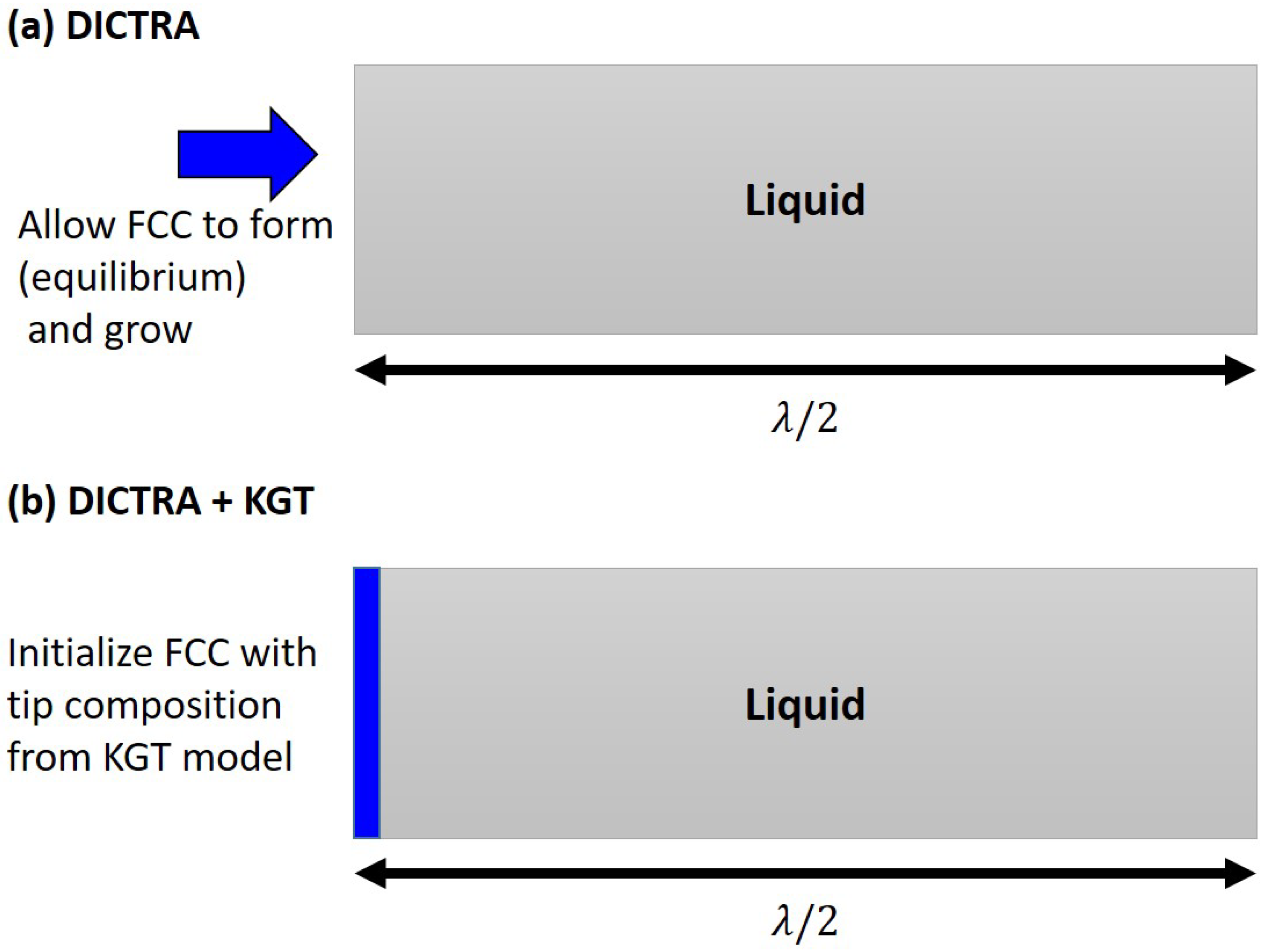
3.2.5. DICTRA-Planar Model

In the DICTRA-Planar method, the DICTRA^® module of Thermo-Calc^® is used. This model considers a one-dimensional closed volume element. It assumes that the interface is planar (Figure 2a) and that there exists a local equilibrium at the interface. Since the calculations are coupled to both thermodynamic and mobility databases, the effect of diffusion in the solid and liquid is considered. The effect of dendrite tip curvature and the kinetic effect at high solidification velocities are ignored. The flux balance at the interface controls the velocity of the interface. The cooling rate from the thermal model is used as input for the model. The solid phase FCC ($\gamma$) given by the equilibrium composition is assumed to nucleate at one end of the domain. The length of the domain is taken as half of the primary dendrite arm spacing (PDAS) due to the symmetry.

3.2.6. DICTRA with KGT Model

In the DICTRA with KGT model, the dendrite tip kinetics is coupled with the DICTRA^® module. All the assumptions of DICTRA-Planar are kept the same, except how the first solid is initialized. DICTRA^® normally calculates the initial solid composition using the equilibrium phase diagram. In this case, the initial solid of an infinitesimal thickness (0.5 nm), with the composition of the dendrite tip ($C_{L,\mathit{tip}}^i\times k_v^i$), is initialized as shown in Figure 2. The simulation started with the temperature corresponding to the tip temperature. This approximation can be rationalized based on the arguments from Tong and Beckermann [14], where they considered that at the dendrite tip, $f_s$ reaches zero. Thus, at the limit ${lim}_{f_s\to 0}{C}_L^i=C_{L,\mathit{tip}}^i$. This approach includes the kinetic effect, dendrite tip kinetics, and finite diffusion in the solid and liquid.

3.2.7. Tong–Beckermann Model

The multicomponent Tong–Beckermann model, based on the diffusion layer concept, accounts for dendrite tip kinetics and finite diffusion in both the solid and liquid [14,15]. A schematic representation of the Tong–Beckermann model is shown in Figure 3.

The model represents the dendritic growth in the direction of the applied thermal gradient (G) and the dendrites are separated by a distance ($\lambda$). Here, only the dendritic envelope is considered. The growth in dendrite, and its representation within the control volume, is given in Figure 3a. The red lines indicate the solute boundary layer that develops around the growing dendrite. Appropriate mass balance equations are written for the control volume in Figure 3b. The velocity of the tip is taken to be the same as the imposed solidification velocity. The velocity of the solid/liquid interface is calculated based on the parabolic cooling assumption [34]. Based on the above assumptions, the set of ordinary differential equations that represent microsegregation is given by the following equations.

$$F_1\left(f_s\right)\frac{d{C}_{L(s/l)}^i}{d{f}_s}=F_2(f_s,C_{L(s/l)}^i,C_{S(s/l)}^i)$$

(11)

where,

$$\begin{array}{cc}\hfill F_1\left(f_s\right)& =2{\beta }^{i^{\prime }}{f}_s(1-H^i\left(f_s\right))\hfill \\ \hfill F_2(f_s,C_{L(s/l)}^i,C_{S(s/l)}^i)& =(1+6{\alpha }^i)(C_o^i-C_{S(s/l)}^i)\hfill \\ \hfill & +(C_{L(s/l)}^i-C_o^i)\left(\frac{H^i\left(f_s\right)}{f_s}-2{\beta }^{i^{\prime }}(1+6{\alpha }^i)(1-H^i\left(f_s\right)\right)\hfill \\ \hfill H^i\left(f_s\right)& =exp\left(-(1-f_s)/(2{\beta }^{{}^{\prime }i}{f}_s)\right)\hfill \end{array}$$

The above equations correspond to the multicomponent extension of the Tong and Beckermann model proposed by Maguin et al. [15]. Here, the solute diffusion is defined via the Fourier number for each species in the solid (${\alpha }^i$) and liquid (${\beta }^i$).

$$\begin{array}{cc}\hfill & {\alpha }^i=\frac{D_S^i{t}_s}{{(\lambda /2)}^2}\hfill \end{array}$$

(12)

$$\begin{array}{cc}\hfill & {\beta }^i=\frac{D_L^i{t}_s}{{(\lambda /2)}^2}\hfill \end{array}$$

(13)

Here, $D_S^i$ and $D_L^i$ are the solute diffusivities of element i in the solid and liquid, respectively. $t_s$ is the solidification time and is taken as the ratio of the solidification interval and the cooling rate. Often, secondary arm spacing is used as the characteristic length in the solid’s Fourier number (${\alpha }^i$) [15]. However, only primary dendrites (cells) form during the LPBF of Haynes 282. Hence, PDAS was taken as the characteristic length for both the solid and liquid Fourier numbers. The mass balance equations do not satisfy the zero flux boundary condition at the symmetry line and a correction factor ($\sigma$) is used. The corrected Fourier number for the liquid is given by Equation (14). The corrected Fourier number is arrived at by solving Equation (11) at the limit of $f_s=0$.

$$\begin{array}{cc}\hfill & {\beta }^{{}^{\prime }i}={\sigma }^i{\beta }^i\hfill \end{array}$$

(14)

$$\begin{array}{cc}\hfill & {\beta }^{{}^{\prime }i}=\frac{C_o^i-C_{S,\mathit{tip}}^i}{2(C_{L,\mathit{tip}}^i-C_o^i)}\hfill \end{array}$$

(15)

Equation (11) is solved for the fraction of solid 0 to 0.99. The ‘odeint’ function of ‘scipy’ was used to solve the equation. The solid and liquid diffusivities, along with the partition coefficients, were calculated using Thermo-Calc^®.

3.2.8. Phase-Field Model

In this current study, a phase-field model simulation was carried out using the Micress^® software [35], which uses the multi-phase-field method [20]. In this report, a two-dimensional (2D) domain taken parallel to the build direction was used as the simulation domain. We assume the “frozen temperature approximation”, that is, the thermal gradient and the cooling rate are constant. These conditions, therefore, depict the evolution of the microstructure in an area that is solidifying under the applied heat conditions at the solidification interface. The simulation starts with a flat solidification interface. Solute diffusion is assumed to be finite in both the solid and liquid. A domain size of 6 µm × 13 µm, with a grid size of 10 nm, is considered and other simulation parameters are the same as used in our previous study [22].

4. Results and Discussion

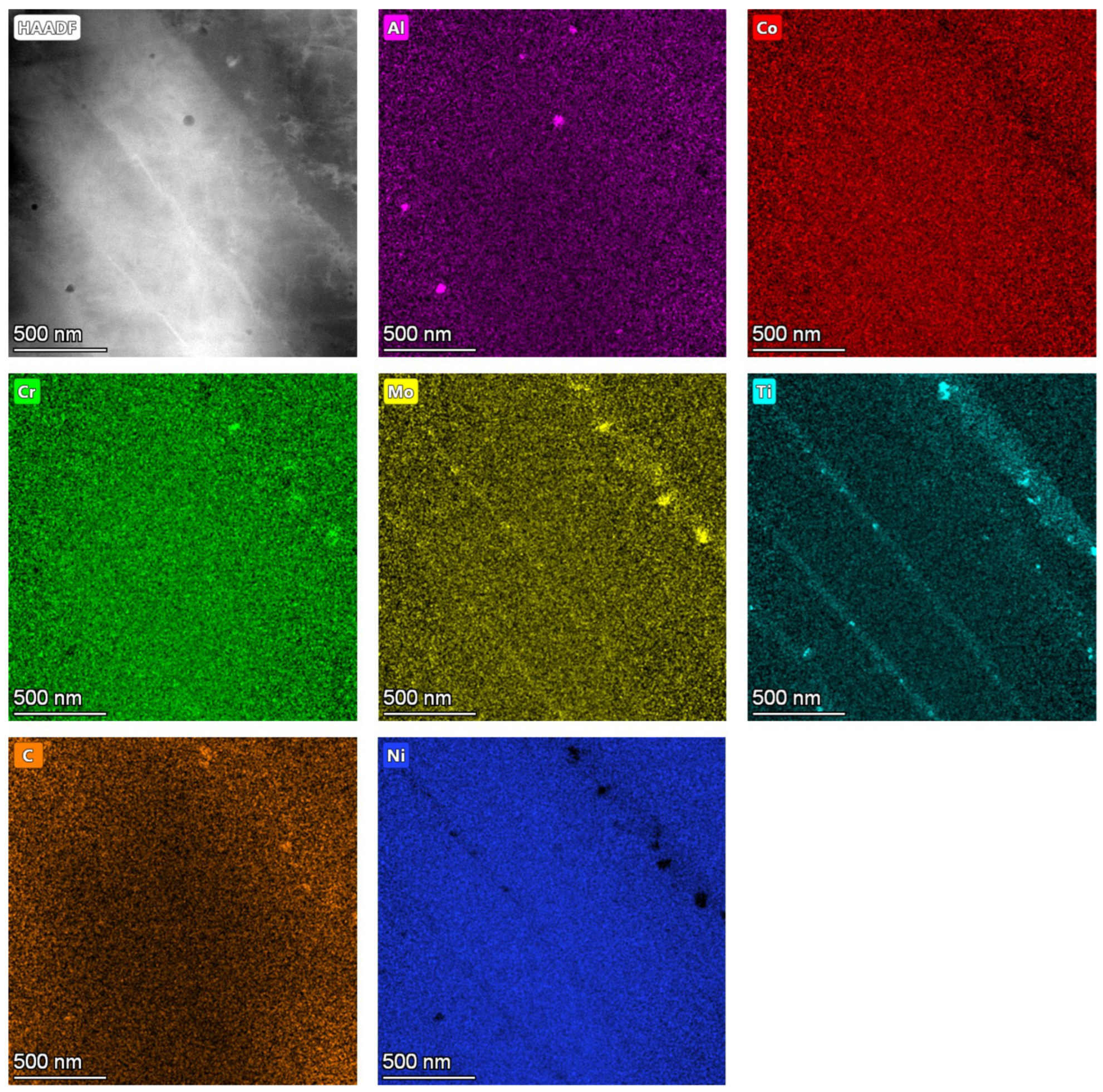
4.1. As-Built Microstructure

The optical micrographs taken perpendicular and parallel to the build direction are shown in Figure 4a,b. The melt pool boundaries can be observed in the optical micrographs. Each grain is etched in a slightly different manner and thus the grains can be seen as regions with different contrast. The secondary electron micrographs, taken at high magnification, indicate the presence of cellular structures and the absence of secondary arms in both the planes that are parallel and perpendicular to the build direction. The cooling rates (≈${10}^6$ K/s) and thermal gradients (≈${10}^7$ K/m) observed in LPBF are very high compared to the values observed in other additive manufacturing techniques [1]. These extreme solidification conditions lead to the presence of only primary dendrites (also called cells). This kind of solidification structure is commonly present under rapid solidification conditions. These structures appear as hexagonal cells if sectioned perpendicular to the growth direction and appear as elongated columns when sectioned parallel to their growth direction. It is clear that the cell spacing is close to 1 µm and agrees with the previously reported values [22].

To understand the solidification behavior, a STEM-EDS map was taken and is shown in Figure 5. From the figure, the segregation of Mo and Ti is evident. The thin elongated regions that are rich in Mo and Ti are the interdendritic regions. Segregation of Mo and Ti to the interdendritic region has been observed in Haynes 282 processed via different manufacturing processes such as welding [36], laser deposition [25], and LPBF [37]. The Mo- and Ti-rich isolated precipitates in interdendritic regions might be MC-type (Ti,Mo)C carbides. These carbides are called primary carbides and are commonly formed during solidification [38]. However, a few isolated bright regions in Mo and Cr might be due to the presence of M₂₃C₆-type Cr₂₃C₆ carbides and M₆C-type Mo₆C carbides [39]. These are secondary carbides and are generally formed after aging heat treatment. These carbides might have formed by the in situ heat treatment effect caused by the thermal cycles. However, further investigation is needed to confirm this claim. Additionally, the interdendritic regions are slightly depleted in Co and Ni. Al and Cr are found to be uniformly distributed in both the dendritic and interdendritic regions. The isolated Al-rich regions might be due to the presence of Al₂O₃ and have been observed during LPBF of IN 718 [40].

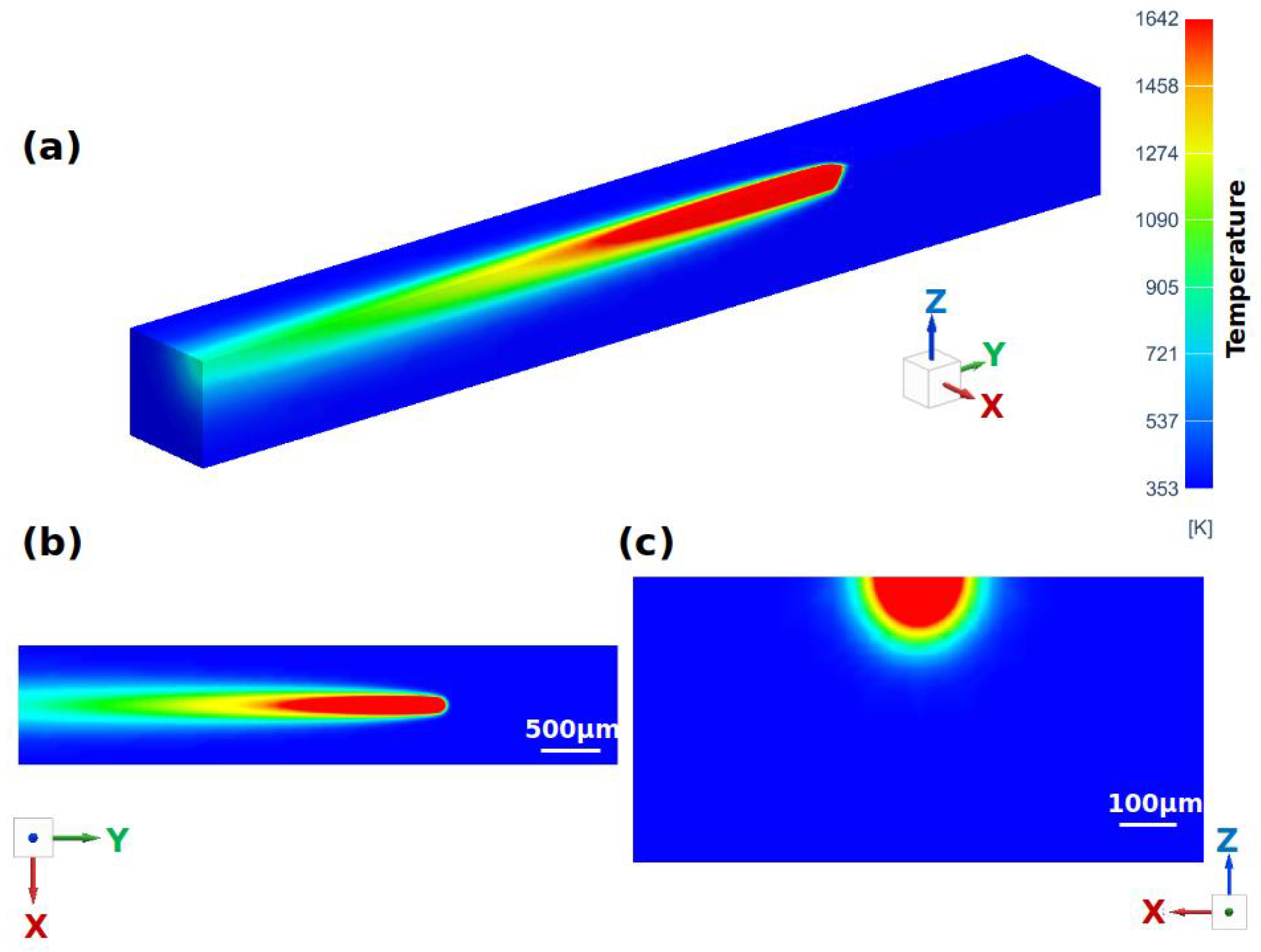
4.2. Thermal Modeling

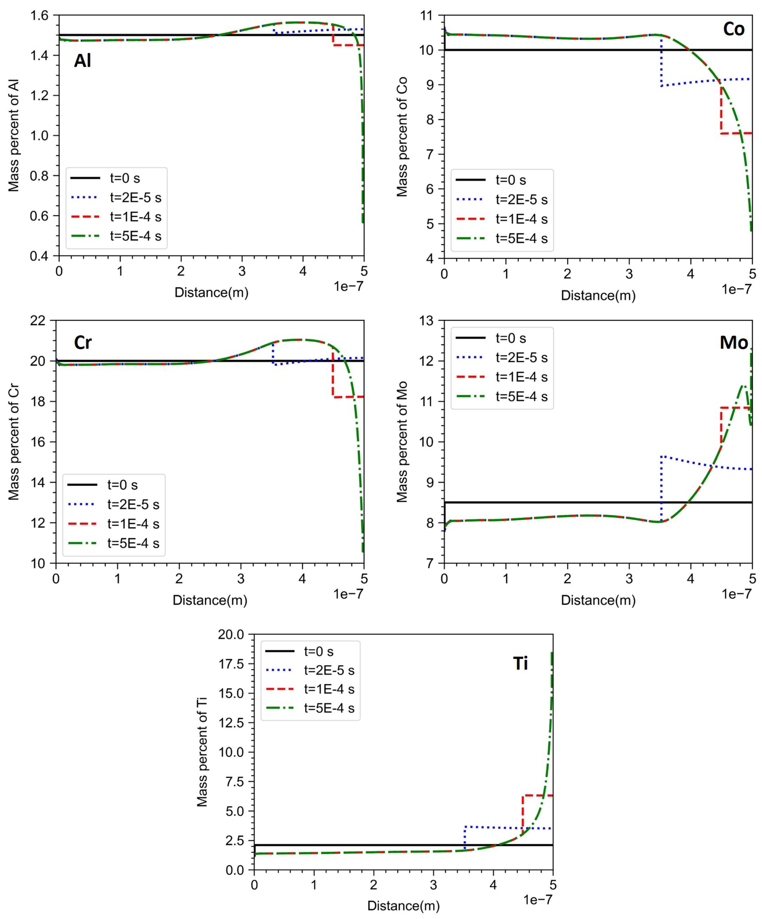
The temperature distribution calculated using the finite element model is shown in Figure 6. The melt pool dimensions are calculated after steady-state is achieved. The melt pool width and depth are 157 µm and 90 µm, respectively. The melt pool dimensions measured from the single-track experiments in the IN 718 alloy match closely with the calculated values [41]. Since the thermophysical properties of IN 718 and Haynes 282 are similar, the melt pool dimensions are also expected to be very close to each other [22]. Moreover, the EOS^® optimized process parameters for Haynes 282 and IN 718 alloys are the same [22].

When the Rosenthal solution or the Eager–Tsai model is used, the width of the melt pool will be approximately twice the melt pool depth due to the semi-circular nature of the melt pool. This is possible when the melting takes place purely by conduction mode [42]. In this case, the melt pool is deeper, suggesting mixed (conduction + keyhole) mode melting [41]. The temperature gradient and cooling rate at the bottom of the melt pool are 1.96 $\times {10}^7$ K/m and 6.92 $\times {10}^5$ K/s, respectively. Thus, the solidification velocity, which is taken as the ratio of the cooling rate and the thermal gradient, is 3.5 cm/s. This solidification velocity, cooling rate, and thermal gradient data will be used for dendrite tip and microsegregation calculations.

4.3. DICTRA-Planar

The domain size is taken as 500 nm based on the experimental observations and previous reports [22]. A cooling rate of 6.92 $\times {10}^5$ K/s, which was calculated from the thermal model, was used for this calculation. The domain is initialized with the liquid having a composition the same as the overall alloy composition.

The evolution of the composition profile with time is given in Figure 7. As time proceeds, the solid–liquid interface moves from left to right. Al and Cr show non-monotonic variation in the composition profile. This non-monotonic variation can be obtained only if the non-diagonal terms in the diffusion matrix are considered [43]. At time $t=2\times {10}^{-5}$ s, one can observe the continuous change in the liquid composition from the solid–liquid interface to the end of the domain. This is due to the finite solute diffusion in liquid. Thus, at the initial stage of solidification, the assumption of complete solute mixing in the liquid is invalid. However, towards the end of solidification ($t=1\times {10}^{-4}$ s), the liquid composition is uniform and the assumption of complete solute mixing of the liquid is valid. From Figure 7, it is clear that the last solidified region is depleted in Al, Co, and Cr, whereas it is enriched in Mo and Ti. In the cases of Mo, Ti, and Co, this matches with the experiments; however, for Cr and Al, they are uniformly distributed in dendritic and interdendritic regions.

4.4. DICTRA-KGT

The material properties needed for calculating the dendrite tip composition and temperature are given in our previous report [31]. The liquid composition ahead of the tip and velocity-dependent partition coefficients are given in

Table 2. Equilibrium and velocity-dependent partition coefficient, along with the liquid composition at the dendrite tip, obtained from KGT model results.

Element	Equilibrium Partition Coefficient	Kinetic Partition Coefficient	Liquid Composition at Tip
Al	1.002	1.002	1.49
Co	1.144	1.143	9.31
Cr	1.005	1.005	19.95
Mo	0.788	0.789	9.88
Ti	0.429	0.431	2.75

. The tip temperature was 1621.51 K. The solid composition for initializing the solid region in the DICTRA with KGT model was calculated as the product of the liquid composition and the partition coefficient. The evolution of the composition profile with time is given in Figure 8.

There are differences between the composition profiles obtained from the DICTRA-Planar and DICTRA with KGT model. From Figure 8, it is clear that near the start of the domain, the composition is different from the equilibrium solid composition. The composition profile remains relatively flat until almost half the domain size, as opposed to the continuous variation observed in the case of DICTRA-Planar. Towards the end of the domain, at the final stage of solidification, the local compositions are close to those obtained from the DICTRA-Planar model. For the same time step ($t=2\times {10}^{-5}$ s), the interface in the DICTRA with KGT model covered 70% of the domain, whereas in the case of the DICTRA-Planar model, the interface covered 20% of the domain. Since the flux balance governs the motion of the interface, the change in the initial condition led to a change in the interface position. A quantitative comparison between both models is given in the subsequent section.

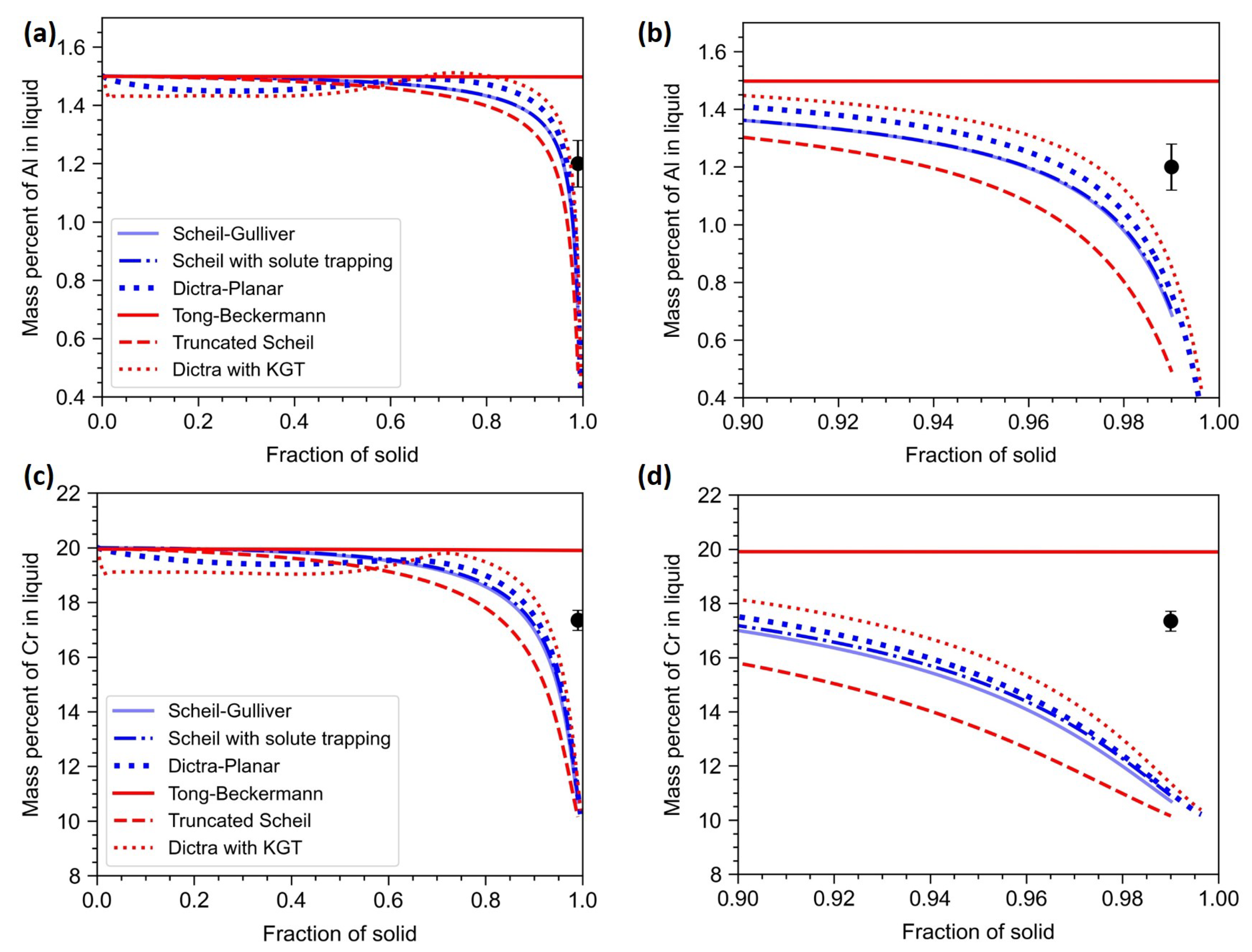
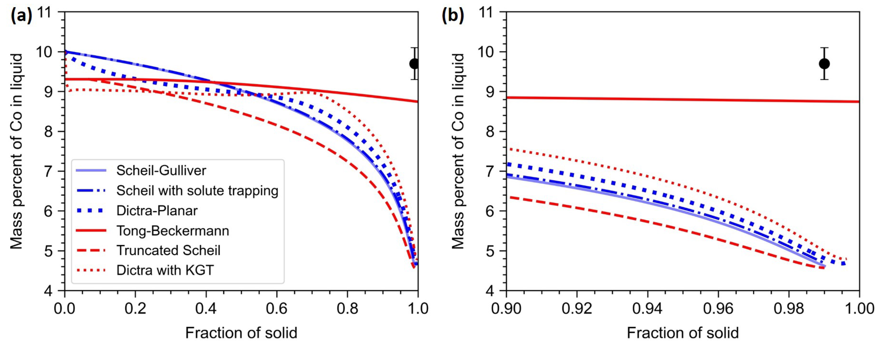
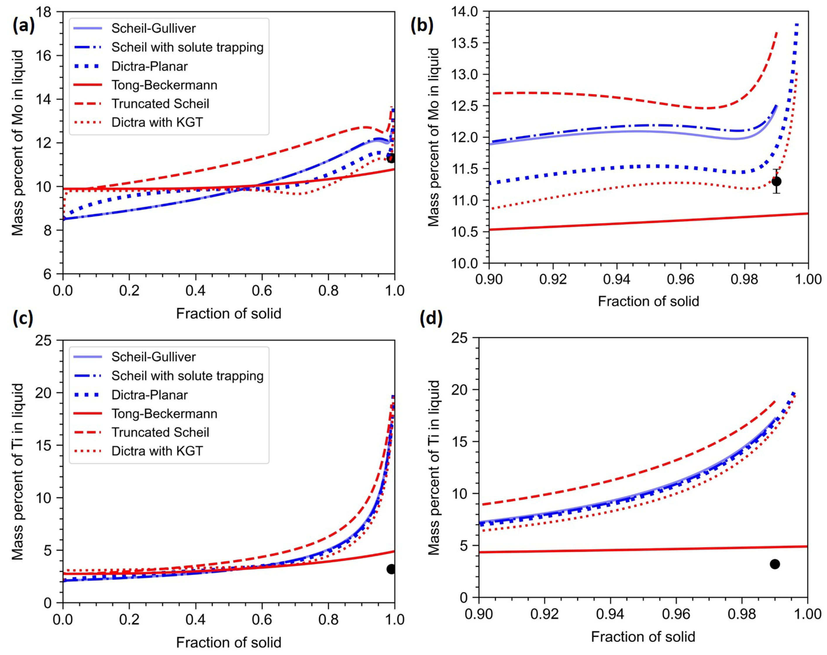
4.5. Model Comparison

In this section, all of the one-dimensional microsegregation models are compared. In Figure 9, the models that account for dendritic tip curvature are plotted in red, whereas the models that assume a planar interface are plotted in blue. The TEM-EDS composition taken at the interdendritic region is considered as the composition at $f_s=0.99$, since it is the last solidifying region. The elements are grouped based on their segregation behavior.

In the case of Al (Figure 9a,b), it is clear that both the Scheil–Gulliver and Scheil with solute trapping models gave the same results. The truncated Scheil model overestimates the segregation behavior. Since the truncated Scheil model assumes a jump condition, the solute is not conserved. The assumption of a jump in the fraction of solid is not physically well-founded and led to discrepancies in the calculation. The incorporation of finite diffusion in the solid and liquid improved the prediction. The inclusion of the curvature effect nudged the results in the correct direction. The Tong–Beckermann model assumes a constant partition coefficient and the partition coefficients of Al and Cr are close to 1.0. Thus, the curve predicted by the Tong–Beckermann model is close to a straight line. A quantitative comparison of the models is given in

Table 3. Comparison of microsegregation models with experiments. Composition (weight%) of the interdendritic region ($f_s=0.99$) is given in the table.

Element	Scheil–Gulliver	Scheil with Solute Trapping	Truncated Scheil	DICTRA-Planar	DICTRA with KGT	Tong–Beckermann	Phase-Field	Experiment
Al	0.69	0.71	0.49	0.76	0.90	1.49	1.42	1.2 ±0.1
Co	4.62	4.69	4.57	4.81	5.05	8.75	8.03	9.7 ± 0.4
Cr	10.7	10.91	10.15	11.0	11.54	19.9	18.36	17.4 ± 0.4
Mo	12.47	12.51	13.67	11.84	11.34	10.76	10.43	11.3 ± 0.2
Ti	17.19	17.01	18.88	16.82	15.78	4.83	5.38	3.2 ± 0.2

.

Co has an equilibrium partition coefficient slightly greater than 1.0. Thus, Co is expected to be depleted in the interdendritic region. As seen from Figure 10, the observations are very similar to that of Al and Cr. Here, the Tong–Beckermann model predicted closer values than other models.

Both Mo and Ti have equilibrium partition coefficients less than 1.0. Thus, they are enriched in the interdendritic region. In the case of Mo (Figure 11a,b), there is a better match with experiments. The effect of solute diffusion is significant and both the DICTRA-Planar and DICTRA with KGT models predict close to the experimental observations, with the DICTRA with KGT model matching more accurately. In the case of Ti (Figure 11c,d), there is a large difference between the predicted and the experimental values. This variation is partly because of the formation of TiC in the interdendritic region. Even after accounting for such phase formation, the discrepancy is too high.

From the above results, it is clear that models incorporating both finite solute diffusion and dendrite tip kinetics resulted in better predictions compared to other models. In the DICTRA with KGT model, the end of the assumed control volume corresponds to the symmetry line between the growing primary dendrite arms. At the terminal stage of solidification, when the boundary layers converge, the zero flux boundary condition cannot be enforced at the symmetry line. This can lead to discrepancies in the prediction. However, this issue is addressed in the Tong–Beckermann model via the correction factor or tuning constant ($\sigma$). These correction factors are calculated from Equations (13) and (14) and are shown in

Table 4. Correction factor for individual elements used in the Tong–Beckermann model.

Element	Correction Factor ($\mathit{\sigma }$)
Al	0.72
Co	0.45
Cr	0.34
Mo	0.54
Ti	0.41

. The correction factors depend only on the overall composition and the dendritic tip characteristics. Thus, the dendrite tip curvature directly influences the microsegregation.

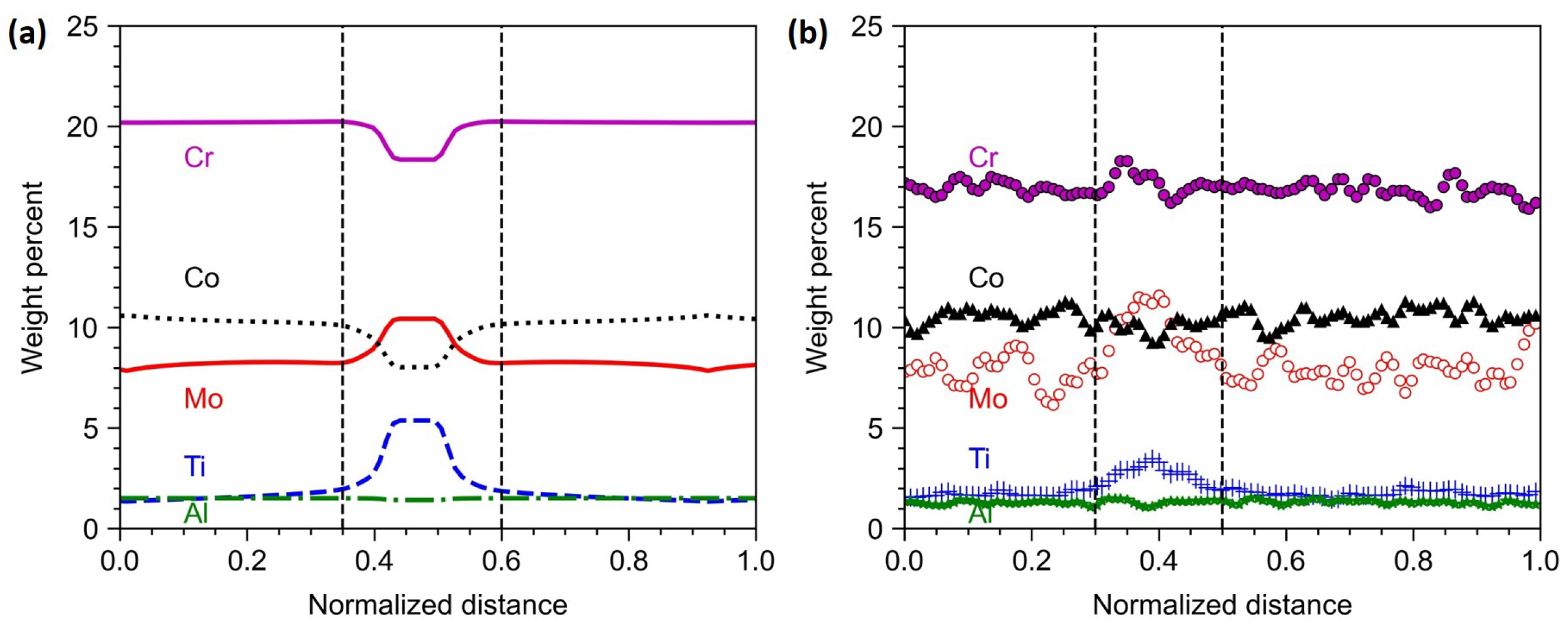
4.6. Phase-Field Model

The evolution of solidification morphologies for the given cooling conditions is given in Figure 12. The liquid phase is shown in red, FCC in white, and the interface is shown in blue. The domain was intialized with a flat solid–liquid interface and the evolution of the interface depends on the imposed thermal conditions. As time proceeds, the flat interface becomes unstable, and undulations are formed. These undulations became cellular perturbations. These perturbations develop into steady-state cellular structures with only primary dendrite arms. This cellular arrangement remained unchanged for the rest of the simulation. The primary dendrite arm spacing is calculated to be approximately 1 µm, which agrees with the experimental value.

The elemental segregation is shown in Figure 13. From the figure, it can be observed that Ti and Mo were enriched in the interdendritic region, while Co and Cr were diminished in the interdendritic region. Al is uniformly distributed. The composition variations across the dendritic and interdendritic regions obtained from the phase-field model and experiments are shown in Figure 14. It is clear that the phase-field model is able to predict the segregation behavior during LPBF of Haynes 282. The overall composition of Cr is slightly lower than the ideal value (20 wt%) and leads to differences in the experimental and simulated values. In all other cases, there is both qualitative and quantitative agreement with the experimental results. This is because most of the physics, such as anisotropic interfacial energies, dendrite curvature effect, and CALPHAD coupling, which were partly or fully ignored in other models, are included in the phase-field model. Thus, one can consider phase-field models as closer to reality, though computationally expensive.

From Table 3 it can be observed that all the Scheil-type models (Scheil–Gulliver, Scheil with solute trapping, and truncated Scheil) overestimated the extent of solute partitioning, as they neglect finite solute diffusion. Incorporation of solute diffusion in both the solid and liquid (DICTRA-Planar model) improved the predictions. Accounting for dendrite tip kinetics in DICTRA led to a marginal improvement in the results. Compositions obtained from the Tong–Beckermann and phase-field model matched closely with the experimentally observed values. Both the models account for dendrite tip kinetics and finite solute diffusion in the solid and liquid, while CALPHAD coupling is only implemented in the phase-field model. The Scheil–Gulliver model, truncated Scheil model, DICTRA-Planar model, and phase-field model are generic and can be applied to any alloy. In the case of models such as the Scheil with solute trapping model and DICTRA with KGT model, the interface response calculations are performed only for a primary solidification phase, and for the rest of the phases the usual assumptions of the Scheil–Gulliver model and DICTRA-Planar model are enforced. Whereas the Tong–Beckermann model is applicable only for alloys solidifying as a single phase.

5. Conclusions

In the current work, microsegregation models with different assumptions on solute diffusion and the nature of the interface are compared with experimentally measured interdendritic composition. Based on the above discussion, the following conclusions can be summarized as follows.

• Incorporation of finite solute diffusion and dendrite tip kinetics improved the model predictions.
• The proposed ‘DICTRA with KGT model’, that couples the dendrite tip calculations and DICTRA^®, matched better with experiments compared to the DICTRA-Planar model.
• Both the multicomponent Tong–Beckermann and the phase-field models gave better predictions than other microsegregation models. These models can be used for accurate prediction of the microsegregation during additive manufacturing.

References

1. DebRoy, T.; Wei, H.; Zuback, J.; Mukherjee, T.; Elmer, J.; Milewski, J.; Beese, A.M.; Wilson-Heid, A.D.; De, A.; Zhang, W. Additive manufacturing of metallic components–process, structure and properties. Prog. Mater. Sci. 2018, 92, 112–224. [Google Scholar] [CrossRef]
2. Babu, S.S.; Raghavan, N.; Raplee, J.; Foster, S.J.; Frederick, C.; Haines, M.; Dinwiddie, R.; Kirka, M.; Plotkowski, A.; Lee, Y.; et al. Additive manufacturing of nickel superalloys: Opportunities for innovation and challenges related to qualification. Metall. Mater. Trans. A 2018, 49, 3764–3780. [Google Scholar] [CrossRef]
3. Hariharan, A.; Lu, L.; Risse, J.; Kostka, A.; Gault, B.; Jägle, E.A.; Raabe, D. Misorientation-dependent solute enrichment at interfaces and its contribution to defect formation mechanisms during laser additive manufacturing of superalloys. Phys. Rev. Mater. 2019, 3, 123602. [Google Scholar] [CrossRef]
4. Sridar, S.; Zhao, Y.; Xiong, W. Phase transformations during homogenization of inconel 718 alloy fabricated by suction casting and laser powder bed fusion: A CALPHAD case study evaluating different homogenization models. J. Phase Equilibria Diffus. 2021, 42, 28–41. [Google Scholar] [CrossRef]
5. Zhang, F.; Levine, L.E.; Allen, A.J.; Stoudt, M.R.; Lindwall, G.; Lass, E.A.; Williams, M.E.; Idell, Y.; Campbell, C.E. Effect of heat treatment on the microstructural evolution of a nickel-based superalloy additive-manufactured by laser powder bed fusion. Acta Mater. 2018, 152, 200–214. [Google Scholar] [CrossRef] [PubMed]
6. Guo, B.; Zhang, Y.; Yang, Z.; Cui, D.; He, F.; Li, J.; Wang, Z.; Lin, X.; Wang, J. Cracking mechanism of Hastelloy X superalloy during directed energy deposition additive manufacturing. Addit. Manuf. 2022, 55, 102792. [Google Scholar] [CrossRef]
7. Rahul, M.; Agilan, M.; Mohan, D.; Phanikumar, G. Integrated experimental and simulation approach to establish the effect of elemental segregation in Inconel 718 welds. Materialia 2022, 26, 101593. [Google Scholar]
8. Fisher, D.; Kurz, W. Fundamentals of Solidification; Trans Tech Publications: Zurich, Switzerland, 1998; pp. 1–316. [Google Scholar]
9. Brody, H.D. Solute Redistribution in Dendritic Solidification. Ph.D. Thesis, Massachusetts Institute of Technology, Cambridge, MA, USA, 1965. [Google Scholar]
10. Clyne, T.; Kurz, W. Solute redistribution during solidification with rapid solid state diffusion. Metall. Trans. A 1981, 12, 965–971. [Google Scholar] [CrossRef]
11. Kraft, T.; Chang, Y. Predicting microstructure and microsegregation in multicomponent alloys. JOM 1997, 49, 20–28. [Google Scholar] [CrossRef]
12. Rappaz, M.; David, S.; Vitek, J.; Boatner, L. Development of microstructures in Fe-15Ni-15Cr single crystal electron beam welds. Metall. Trans. A 1989, 20, 1125–1138. [Google Scholar] [CrossRef]
13. Flood, S.; Hunt, J. A model of a casting. Appl. Sci. Res. 1987, 44, 27–42. [Google Scholar] [CrossRef]
14. Tong, X.; Beckermann, C. A diffusion boundary layer model of microsegregation. J. Cryst. Growth 1998, 187, 289–302. [Google Scholar] [CrossRef]
15. Maguin, V.; Guillemot, G.; Jaquet, V.; Niane, N.; Rougier, L.; Daloz, D.; Zollinger, J.; Gandin, C.A. Finite diffusion microsegregation model applied to multicomponent alloys. In IOP Conference Series: Materials Science and Engineering; IOP Publishing: Bristol, UK, 2019; Volume 529, p. 012029. [Google Scholar]
16. Boettinger, W.J.; Kattner, U.R.; Banerjee, D.K. Analysis of solidification path and microsegregation in multicomponent alloys. In Modelling of Casting, Welding and Advanced Solidification Processed—VIII; The Minerals, Metals & Materials Society: Pittsburgh, PA, USA, 1998; Volume 1, pp. 159–170. [Google Scholar]
17. Keller, T.; Lindwall, G.; Ghosh, S.; Ma, L.; Lane, B.M.; Zhang, F.; Kattner, U.R.; Lass, E.A.; Heigel, J.C.; Idell, Y.; et al. Application of finite element, phase-field, and CALPHAD-based methods to additive manufacturing of Ni-based superalloys. Acta Mater. 2017, 139, 244–253. [Google Scholar] [CrossRef]
18. Borgenstam, A.; Höglund, L.; Ågren, J.; Engström, A. DICTRA, a tool for simulation of diffusional transformations in alloys. J. Phase Equilibria 2000, 21, 269–280. [Google Scholar] [CrossRef]
19. Thermo-Calc Software AM. Thermo-Calc. 2021. Available online: https://thermocalc.com/ (accessed on 31 March 2023).
20. Eiken, J. A Phase-Field Model for Technical Alloy Solidification; Shaker: Maastricht, Germany, 2009. [Google Scholar]
21. Agilan, M.; Satyamshreshta, K.; Sivakumar, D.; Phanikumar, G. High-Throughput Experiment and Numerical Simulation to Study Solidification Cracking in 2195 Aluminum Alloy Welds. Metall. Mater. Trans. A 2022, 53, 1906–1918. [Google Scholar] [CrossRef]
22. Hariharan, V.; Pramod, S.; Kesavan, D.; Murty, B.; Phanikumar, G. ICME framework to simulate microstructure evolution during laser powder bed fusion of Haynes 282 nickel-based superalloy. J. Mater. Sci. 2022, 57, 9693–9713. [Google Scholar] [CrossRef]
23. Pike, L. HAYNES® 282 alloy: A new wrought superalloy designed for improved creep strength and fabricability. In Proceedings of the Turbo Expo: Power for Land, Sea, and Air, Barcelona, Spain, 8–11 May 2006; American Society of Mechanical Engineers: New York, NY, USA, 2006; Volume 42398, pp. 1031–1039. [Google Scholar]
24. Hariharan, V.; Kaushik, R.; Phanikumar, G.; Murty, B. Tailoring the Crystallographic Texture of Laser Powder Bed Fused Haynes 282 Through Scan Rotation Modification: Simulation & Experiments. SSRN 2023. [Google Scholar] [CrossRef]
25. Ramakrishnan, A.; Dinda, G. Microstructure and mechanical properties of direct laser metal deposited Haynes 282 superalloy. Mater. Sci. Eng. A 2019, 748, 347–356. [Google Scholar] [CrossRef]
26. Haynes International. 2022. Available online: https://haynesintl.com/docs/default-source/pdfs/new-alloy-brochures/high-temperature-alloys/brochures/282-brochure.pdf (accessed on 15 March 2023).
27. Siemens Digital Industries Software Simcenter 3D. 2022. Available online: https://plm.sw.siemens.com/en-US/simcenter/mechanical-simulation/3d-simulation/ (accessed on 15 March 2023).
28. Wu, C.; Wang, H.G.; Zhang, Y.M. A new heat source model for keyhole plasma arc welding in FEM analysis of the temperature profile. Weld. J. N. Y. 2006, 85, 284. [Google Scholar]
29. Aziz, M.J.; Kaplan, T. Continuous growth model for interface motion during alloy solidification. Acta Metall. 1988, 36, 2335–2347. [Google Scholar] [CrossRef]
30. Kurz, W.; Giovanola, B.; Trivedi, R. Theory of microstructural development during rapid solidification. Acta Metall. 1986, 34, 823–830. [Google Scholar] [CrossRef]
31. Hariharan, V.S.; Murty, B.S.; Phanikumar, G. Interface Response Functions for multicomponent alloy solidification—An application to additive manufacturing. arXiv 2023, arXiv:2303.07663. [Google Scholar] [CrossRef]
32. Virtanen, P.; Gommers, R.; Oliphant, T.E.; Haberland, M.; Reddy, T.; Cournapeau, D.; Burovski, E.; Peterson, P.; Weckesser, W.; Bright, J.; et al. SciPy 1.0: Fundamental Algorithms for Scientific Computing in Python. Nat. Methods 2020, 17, 261–272. [Google Scholar] [CrossRef]
33. Haines, M.; Plotkowski, A.; Frederick, C.L.; Schwalbach, E.J.; Babu, S.S. A sensitivity analysis of the columnar-to-equiaxed transition for Ni-based superalloys in electron beam additive manufacturing. Comput. Mater. Sci. 2018, 155, 340–349. [Google Scholar] [CrossRef]
34. Giovanola, B.; Kurz, W. Modeling of microsegregation under rapid solidification conditions. Metall. Trans. A 1990, 21, 260–263. [Google Scholar] [CrossRef]
35. Access e.V. Micress 7.1. 2022. Available online: https://micress.rwth-aachen.de/ (accessed on 15 March 2023).
36. Osoba, L.; Ding, R.; Ojo, O. Microstructural analysis of laser weld fusion zone in Haynes 282 superalloy. Mater. Charact. 2012, 65, 93–99. [Google Scholar] [CrossRef]
37. Shaikh, A.S.; Schulz, F.; Minet-Lallemand, K.; Hryha, E. Microstructure and mechanical properties of Haynes 282 superalloy produced by laser powder bed fusion. Mater. Today Commun. 2021, 26, 102038. [Google Scholar] [CrossRef]
38. Matysiak, H.; Zagorska, M.; Andersson, J.; Balkowiec, A.; Cygan, R.; Rasinski, M.; Pisarek, M.; Andrzejczuk, M.; Kubiak, K.; Kurzydlowski, K.J. Microstructure of Haynes® 282® superalloy after vacuum induction melting and investment casting of thin-walled components. Materials 2013, 6, 5016–5037. [Google Scholar] [CrossRef]
39. Joseph, C.; Persson, C.; Hörnqvist Colliander, M. Precipitation kinetics and morphology of grain boundary carbides in Ni-base superalloy Haynes 282. Metall. Mater. Trans. A 2020, 51, 6136–6141. [Google Scholar] [CrossRef]
40. Xu, J.; Ma, T.; Peng, R.L.; Hosseini, S. Effect of post-processes on the microstructure and mechanical properties of laser powder bed fused IN718 superalloy. Addit. Manuf. 2021, 48, 102416. [Google Scholar] [CrossRef]
41. Pramod, S.; Kesavan, D. Melting modes of laser powder bed fusion (L-PBF) processed IN718 alloy: Prediction and experimental analysis. Adv. Ind. Manuf. Eng. 2023, 6, 100106. [Google Scholar] [CrossRef]
42. Promoppatum, P.; Yao, S.C.; Pistorius, P.C.; Rollett, A.D. A comprehensive comparison of the analytical and numerical prediction of the thermal history and solidification microstructure of Inconel 718 products made by laser powder-bed fusion. Engineering 2017, 3, 685–694. [Google Scholar] [CrossRef]
43. Guillemot, G.; Senninger, O.; Hareland, C.A.; Voorhees, P.W.; Gandin, C.A. Thermodynamic coupling in the computation of dendrite growth kinetics for multicomponent alloys. Calphad 2022, 77, 102429. [Google Scholar] [CrossRef]
Figure 1. Models used in this study and the effects considered in each model.
Crystals 13 00842 g001
Figure 2. A schematic representation of the DICTRA-Planar and DICTRA with KGT models.
Crystals 13 00842 g002
Figure 3. A schematic representation of (a) columnar dendritic growth along with symmetry line, (b) control volume (inspired from [14]).
Crystals 13 00842 g003
Figure 4. Optical micrograph of the as-built sample taken (a) along and (b) perpendicular to the build direction. Secondary electron micrographs showing cellular structures taken (c) along and (d) perpendicular to the build direction.
Crystals 13 00842 g004
Figure 5. STEM-EDS map showing the dendritic and interdendritic regions.
Crystals 13 00842 g005
Figure 6. (a) Trimetric view showing the melt pool and the temperature distribution. (b) Top view showing the length and width of the melt pool. (c) Cross section showing the melt pool width and depth.
Crystals 13 00842 g006
Figure 7. Evolution of composition profile with time as predicted by the DICTRA-Planar model.
Crystals 13 00842 g007
Figure 8. Evolution of the composition profile with time as predicted by the DICTRA with KGT model.
Crystals 13 00842 g008
Figure 9. (a,b) Comparison of predictions from different microsegregation models for Al. (c,d) Comparison of predictions from different microsegregation models for Cr.
Crystals 13 00842 g009
Figure 10. (a) Comparison of predictions from different microsegregation models for Co. (b) Microsegregation plot shown at the end of the solidification.
Crystals 13 00842 g010
Figure 11. (a,b) Comparison of predictions from different microsegregation models for Mo. (c,d) Comparison of predictions from different microsegregation models for Ti.
Crystals 13 00842 g011
Figure 12. Microstructure evolution during LPBF.
Crystals 13 00842 g012
Figure 13. Elemental segregation during solidification.
Crystals 13 00842 g013
Figure 14. Composition variation across the dendritic and interdendritic regions obtained from (a) phase-field model, and (b) TEM-EDS line scan.
Crystals 13 00842 g014