Abstract
The Gleeble-3800 thermal simulator was used to perform hot compression experiments on Q345 steel at a temperature of 1123~1373 K, a strain rate of 0.01~10 s−1, and 60% deformation. Analysis of the flow curves of Q345 steel revealed that flow stress decreases with the increase of deformation temperature and decrease of strain rate. According to the stress–strain curve of Q345 steel, three constitutive models of Johnson–Cook, Modified Johnson–Cook and strain-compensated Arrhenius were established. By comparison, it was found that the strain-compensated Arrhenius model has higher accuracy, and its correlation coefficient and average relative error are 0.995 and 4.93%, respectively. In addition, the thermal processing map of Q345 steel was established, and the optimal processing range was temperature 1253–1373 K, strain rate 0.5–10 s−1.
1. Introduction
Q345 steel, recognized by the international and American corresponding alloy grades as E355CC and A572(345) Gr50, respectively, is a type of low-carbon light microalloy steel with the largest output and a wide application. Due to its outstanding characteristics such as its good comprehensive thermodynamic properties, corrosion resistance, processing stability, and steel welding firmness, it is widely used in building bridge structures, ship unloading boxes, oil tank boxes, hoisting machinery, bridge structures, etc. The manufacturing process of Q345 steel is mainly in the state of high temperature hot rolling or normalizing [1,2,3,4]. At present, a large number of scholars have studied the mechanical properties of Q345 steel under a high temperature tension and compression state [5,6]. However, due to the complexity of metal in the hot deformation process, the effects of strain, strain rate, and temperature on its flow stress cannot be described accurately and reliably by the material constitutive model. Therefore, it is necessary to compare and analyze different constitutive models for the widely-used Q345 steel [1].
The constitutive equation is used to describe the relationship between flow stress and strain, strain rate, and temperature. It can guide the finite element simulation, determine the ideal parameters of thermal processing, and assist to guide the manufacturing process. At present, the constitutive models including Johnson–Cook [7] and Arrhenius [8,9] often describe the thermal deformation characteristics of materials. To be more specific, the JC model is extensively used to explain the thermal deformation behavior of alloys on account of the simplicity of its multiplicative form, while the Arrhenius type formula proposed by Sellars and McTegart expresses the flow stress according to the law of hyperbolic sine, which has been improved many times and can be applied to the high temperature rheological behavior of various alloys. Sahu et al. [10] studied the elastic–plastic deformation behavior of AA1100 aluminum alloy at strain rate by a uniaxial tensile test and modeled by the Johnson–Cook constitutive equation. The results showed that the flow stress predicted by the equation was consistent with the test value, and the stress variation trend was the same. The simulation results showed that the calculated compressive stress–strain curve was consistent with the experimental curve, which indicates the validity and feasibility of the JC model in finite element calculation. Bobbili et al. [11] conducted SHPB compression bar tests on FeCoNiCr high-entropy composites and established a Modified Johnson–Cook model with a strain rate ranging from 0.01 to 3500, which has high accuracy and universal construction methods. Yang [12] and others applied the Arrhenius constitutive model to study the hot compression deformation behavior of LSFed TC4 alloy, and the results showed that the predicted values were basically consistent with the experimental values, with average relative errors of 10.4% (800–950 °C) and 8.3% (650–800 °C), respectively. The results proved that the Arrhenius model had a higher level of precision. Therefore, it is of great significance to study the thermal deformation behavior and constitutive models by means of a thermal simulation test, so as to select the model with the highest accuracy.
In this study, the hot compression test of Q345 steel was carried out and the hot deformation behavior of Q345 steel was analyzed. Three constitutive models, namely, the Johnson–Cook model, the Modified Johnson–Cook model, and the strain-compensated Arrhenius model, were used to predict its high-temperature flow stress. In addition, the thermal processing map of Q345 steel was established, providing reliable data support and theoretical reference for the research of the hot working forming technology of this steel.
2. Materials and Methods
The chemical composition of the Q345 carbon cylindrical sample with a size of Φ10 mm × 15 mm is shown in Table 1. After polishing the sample, the hot compression experiment was performed on the Gleeble-3800 simulation testing machine (Dynamic Systems Inc., New York, NY, USA). In order to reduce the friction during the deformation process, the two ends of the sample were polished smoothly with a metal tantalum sheet and lubricated with graphite lubricant. A vacuum was drawn to prevent oxidation of the sample at the same time. The compression test conditions were as follows: the deformation temperature was 1123~1373 K; the interval was 50 K; the strain rates: 0.01, 0.1, 1, and 10 s−1; and the true strain was 0.92. The experimental process is shown in Figure 1.

Table 1.
Chemical composition of Q345 steel (wt/%).
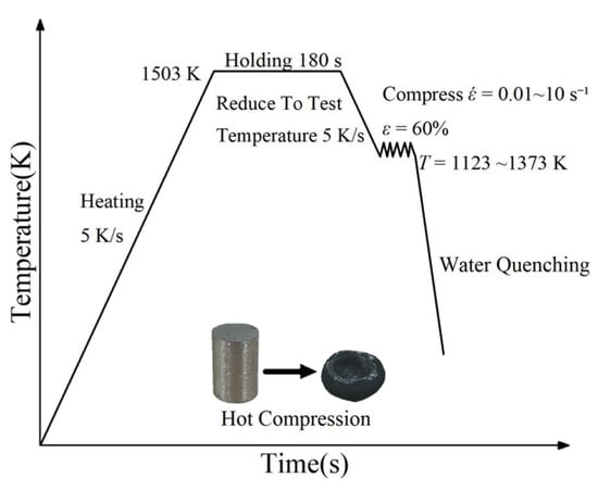
Figure 1.
Schematic diagram of single-pass compression experiment.
3. Results and Discussion
3.1. Stress–Strain Curve Analysis
Figure 2 exhibits the stress–strain curve of Q345 steel at different strain rates. The stress decreases as the temperature increases at the same strain rate. Since the thermal vibration of metal atoms intensifies with the increase of temperature, this promotes all the movements requiring the rearrangement of small atoms, such as dislocations and grain boundaries. Therefore, dislocations are easier to move, which enhances dislocation annihilation and recovery, resulting in dynamic softening. Or, more likely, the boundary mobility dominating recrystallization destroys dislocations and restores grain boundary order, reducing the energy storage of microstructure, which can also result in dynamic softening. The deformation process of metal is mainly divided into three stages: The first stage is when the work hardening stage occurs due to the increase of dislocation density [13], and the increase of strain is accompanied by a rapid increase in flow stress. The second stage is the transitional stage. As the strain increases, the rate of flow stress rise slows down until it reaches the peak. The softening and work hardening caused by dynamic recrystallization compete with each other until the two finally reach equilibrium. In the third softening stage, the stress–strain curve tends to be stable, and the increase of dislocations enhances the dominance of dynamic recrystallization.
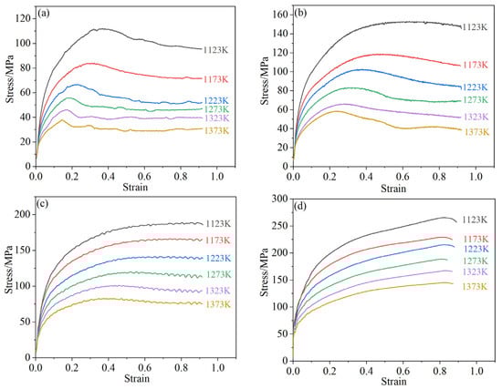
Figure 2.
True stress–true strain curves of Q345 steel at different strain rates: (a) 0.01 s−1; (b) 0.1 s−1; (c) 1 s−1; (d) 10 s−1.
As shown in Figure 2a–c, at the same temperature, the increase of strain gradually lowers the flow stress and eventually stabilizes because the softening effect produced by dynamic recovery gradually offsets the work hardening that resulted from the dislocation proliferation effect. Since the atoms do not have enough time to diffuse at a high strain rate (10 s−1), the dynamic recrystallization behavior is not fully carried out due to insufficient energy accumulation. Meanwhile, the flow stress continues to increase, and no steady-state stress appears. These two curves with different changing trends reflect that Q345 steel undergoes different degrees of dynamic recrystallization during hot deformation at different strain rates [14].
3.2. Johnson–Cook Constitutive Model
The Johnson–Cook model is as follows:
where: is the flow stress (MPa), ε is true strain, is the dimensionless strain rate, is strain rate (), refers to the reference strain rate (), A refers to the yield stress at the reference temperature and rate, B refers to the strain hardening coefficient, n refers to the strain-hardening index, and [15]. T is the temperature (K), is the melting temperature (1673 K), and is a reference temperature (T ≥ ). C and m represent the strain rate hardening coefficient and thermal softening index, respectively. Based on existing studies, the reference temperature is 1123 K, and the reference strain rate is 1 to determine the parameters in the equation. Equation (1) can be expressed as:
Under such deformation conditions, the yield stress is A = 150.95 MPa. The relationship between ln and ln() can be obtained by substituting the value of A into Equation (2), as depicted in Figure 3a. Then the values of B and n are 45.68 MPa and 0.766, respectively, from the fitting curve.
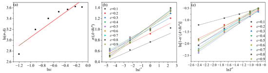
Figure 3.
Relationship between: (a) ln and ln() at 1123 K and 1; (b) at 1123 K; (c).
When the deformation temperature is 1123 K, Equation (1) can be transformed into Equation (3):
The C value obtained by fitting the slope is 0.103, as shown in Figure 3b.
In the same way, when the strain reference rate is 1.0, =0, Equation (1) can be transformed into Equation (4):
The relationship between ln and ln at different temperatures under a specific strain can be obtained from Equation (4). Then, the average m value, 0.904, was generated by the slope of the linear fitting curve, as depicted in Figure 3c.
Table 2 shows the Johnson–Cook model parameters of Q345. The constitutive equation is as follows:
Table 2.
Parameters for the Johnson–Cook model.
The predicted flow stress value of the Johnson–Cook model is compared with the experimental value, as illustrated in Figure 4 and Table 3. Under the same deformation condition, it has obvious error. The maximum absolute error, 42.61 MPa, appeared at 1323 K/0.1. The mean absolute error showed a trend of first rise and then decline with increasing temperature. With the increase of rheological rate, the mean absolute error decreased notably, and the error was mainly concentrated in the low strain rate (0.1).
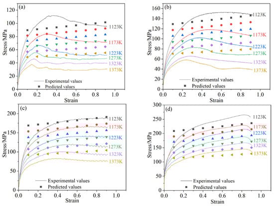
Figure 4.
Comparison between predicted and experimental flow stress using Johnson–Cook model at different strain rates: (a) 0.01 s−1; (b) 0.1 s−1; (c) 1 s−1; (d) 10 s−1.
Table 3.
Absolute error mean value and relative error mean value of three kinds of constitutive models under different deformation conditions.
3.3. Modified Johnson–Cook Constitutive Model
The Modified Johnson–Cook model is expressed as follows:
In the equation: and is the material constant, , and the meaning of other parameters is the same as Equation (1) [16,17].
When the reference temperature is 1123 K and the strain rate is 1.0 s−1, Equation (6) can be transformed into Equation (7):
Substituting the flow stress under this deformation condition into Equation (7), the obtained scatter plot was fitted with a third-degree polynomial. As shown in Figure 5a, the fitting coefficients and were 88.42375 MPa, 403.34968 MPa, −564.06091 MPa, and 266.96535 MPa, respectively.
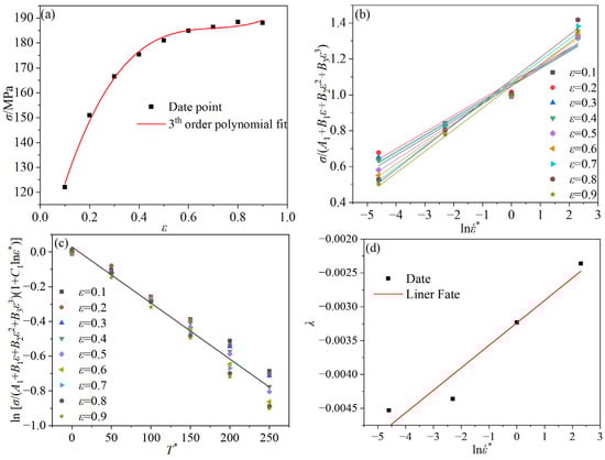
Figure 5.
Relationship between: (a) and at 1123 K and 1; (b) and at the temperature of 1123 K; (c) and at 1; (d) and .
When the reference temperature is 1123 K, Equation (6) can be transformed into Equation (8):
The value of can be obtained from the − relationship diagram. As illustrated in Figure 5b, the value was 0.10659.
In order to simplify the equation, a new parameter is introduced. Equation (6) can be changed to Equation (9):
The value is taken as the mean value of different true strains (0.1~0.9). Selecting a specific strain, the and relationship diagram of different deformation temperatures and strain rates were obtained as shown in Figure 5c. Then, the values of 4 different strain rates can be obtained from the slope of the linear fitting curve.
The values of and can be obtained from the − relationship graph. The relationship between and is shown in Figure 5d.
Using the Modified Johnson–Cook model, the material parameters of Q345 are shown in Table 4.
Table 4.
Calculated Modified Johnson–Cook model coefficients.
The Modified Johnson–Cook constitutive equation is as follows:
Using the above constitutive equation, the predicted value of the flow stress of the model under different deformation conditions can be obtained, which was compared with the experimental value of the flow stress under this condition, and the result is shown in Figure 6. The average absolute error of the Modified Johnson–Cook model is shown in Table 3.
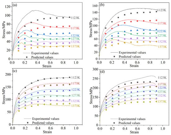
Figure 6.
Comparison between predicted and experimental flow stress using Modified Johnson–Cook model at different strain rates: (a) 0.01 s−1; (b) 0.1 s−1; (c) 1 s−1; (d) 10 s−1.
Figure 6 presents that at higher deformation temperatures (1223, 1273, 1323, and 1373 K) and low strain rates (0.01, 0.1, and 1 ), the predicted flow stress of the Modified Johnson–Cook model is in good agreement with the experimental value. It can be seen from Table 3 that under the same deformation conditions, the deviation between the predicted value and the experimental value was relatively small. The maximum absolute error average appeared at 1223 K, 10 , which was 32.48 MPa. The larger mean absolute errors were concentrated in strain rates of 0.01 and 10 . When the strain rate was 0.01 , the mean absolute error fluctuated greatly as the temperature increased. Overall, the Modified Johnson–Cook model is more accurate than the Johnson–Cook model.
3.4. Strain-Compensated Arrhenius Constitutive Model
The Arrhenius constitutive model is a model commonly used to describe the relationship between deformation rate, temperature, and stress–strain during high-temperature deformation of materials [18,19]. The equation is expressed as follows:
Among them, R is the gas constant value is 8.314 J/(mol·K), Q is the thermal deformation activation energy, A, and is the material constant.. The first two equations of Equation (12) represent the low stress conditions (ασ < 0.8) and high stress conditions (ασ > 1.2), respectively. The hyperbolic sine function in the third equation is a more general relation covering a wider stress range [8]. Therefore, this paper used the hyperbolic sine function to describe the thermal deformation behavior of Q345 steel.
The values of can be obtained by the relationship between and respectively, while the value of Q can be product of R and the slopes of − and /T − . The above relations are shown in Figure 7.
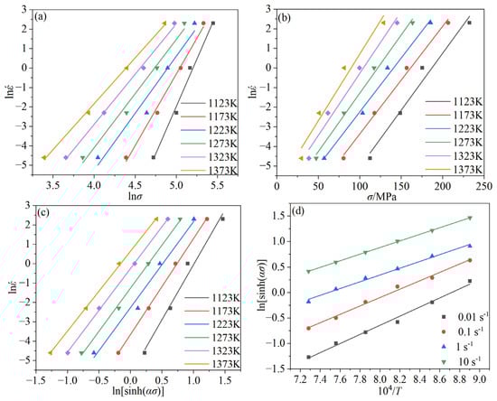
Figure 7.
Relationship between: (a); (b); (c) − ; (d)/T − .
In this paper, the Zener–Hollomon parameter is introduced, which comprehensively reflects the influence of deformation temperature and strain rate on the thermal deformation behavior of metals. Zener–Hollomon parameters are expressed as:
According to Equation (13), the values of n and A can be obtained from the relationship between lnZ and ln[sinh (ασ)], as shown in Figure 8.
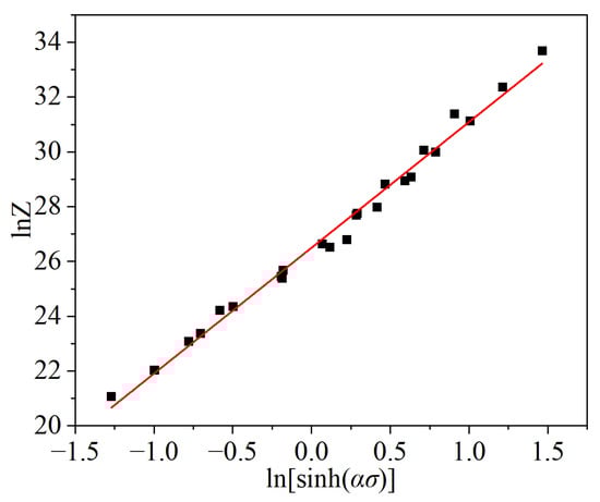
Figure 8.
Relationship between lnZ and .
Combining Equation (11) with Equation (13), the explicit form of stress is obtained:
Under high temperature conditions, strain not only has a significant effect on flow stress, but also on the material constant ( and lnA), which is a polynomial function of strain in the entire strain range, such as Equation (15), which introduces the influence of strain on the constitutive equation.
We performed multi-order polynomial fitting on and lnA, and the results are shown in Figure 9. The coefficients of the fitted polynomial are shown in Table 5.
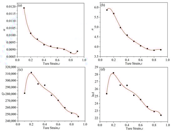
Figure 9.
Relationships between material parameters and : (a) α; (b) n; (c) Q; (d) lnA.
Table 5.
Coefficients of the polynomial for α, n, Q and lnA.
The coefficient of each term in Equation (15) can be calculated as shown in Table 5, from which the sum A value at any deformation temperature and deformation rate can be derived and then the flow stress value can be calculated.
It can be seen from Figure 10 that at a high temperature (1273, 1323, 1373 K) and low strain rate (0.01, 0.1, 1 ), the difference between the flow stress value predicted by the strain-compensated Arrhenius model and the experimental stress value was small. It can also be concluded from Table 3 that under most deformation conditions, the deviation between the predicted value and the measured value was small. The maximum absolute error average appeared at 1123 K,1 , which was 15.2 MPa. As the temperature rose, the mean absolute error generally showed a downward trend. Overall, the error was mainly concentrated in the high strain rate (10 ).
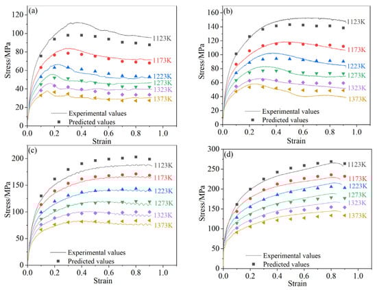
Figure 10.
Comparison between predicted and experimental flow stress using Strain-compensated Arrhenius model at different strain rates: (a) 0.01 s−1; (b) 0.1 s−1; (c) 1 s−1; (d) 10 s−1.
3.5. Precision Analysis
From the above calculation results, it can be noticed that the Johnson–Cook model only obtained relatively accurate prediction values at the reference temperature (1123 K). Shayanpoor [20] et al. mentioned that the JC model is not suitable for high temperature and low strain rate conditions, and the model is more suitable for high strain rate conditions at room temperature. The results reveal that the JC model could only predict flow stress in the narrow region of reference temperature and reference strain rate. To some extent, the primary reason is that the model only considers the work hardening effect, strain rate effect, and temperature effect, but neglects the interaction of the three in the actual deformation process. However, different from the definition of JC model, the thermal softening index m of metal Q345 steel is related to strain and strain rate. In addition, its strain rate hardening C is directly proportional to the change of temperature. This shows that the high temperature rheological behavior of metal Q345 is controlled by more than the three independent phenomena of thermal softening, strain rate hardening, and strain hardening that are required by the JC model. Moreover, the coupling effects of strain and temperature, strain rate and temperature should be considered. Therefore, when the prediction parameters are far from the reference temperature and strain rate used to evaluate the constants, the JC model cannot include these coupling effects, so the error of the prediction value increases. The Modified Johnson–Cook model can better predict the high temperature deformation behavior of Q345 steel. However, the MJC model only improves the fit of the JC model from the perspective of strain hardening and thermal softening, and the effect is not obvious, especially under the condition of low strain rate with strong recrystallization. No significant improvement in terms of practicability has been noticed, since MJC does not consider the recrystallization effect nor the recovery of dislocation density.
In order to further compare the accuracy of the three constitutive models, the correlation coefficient R, the absolute value of the average relative error AARE, and the relative error RE are used to quantitatively analyze the accuracy of the corresponding variable compensation constitutive equation. The Equations (16)−(18) of these parameters are as follows.
where and are the experimental and predicted flow stress (MPa), respectively. and are the average values of and , respectively. N is the total number of data used in this study.
The mean values of relative errors of the predicted values under each condition of the three constitutive equations are shown in Table 3. The RE value of JC model varied from −62.18% to 5.65%, and the average RE value was −17.09%. The RE value of MJC model varied from −4.27% to 16.32%, and the average value was 6.38%. The RE of the Strain-compensated Arrhenius model varied from −8.84% to 8.30%, with an average value of 0.2%. Thus, the Strain-compensated Arrhenius model shows the highest accuracy. According to Equation (17), the correlation coefficients of the Johnson–Cook model, the Modified Johnson–Cook model and the Strain-compensated Arrhenius model were 0.96989, 0.98844 and 0.99644, respectively. Figure 11 shows the correlation between the experimental flow stress and the predicted flow stress of the three models. It can be seen that most of the data points are close to the regression line. The correlation coefficient R is usually used to express the linear correlation between the experimental value and the predicted value, but it has a certain deviation in evaluating the predictive ability. Therefore, AARE is used as an unbiased statistical parameter to further determine the predictability of the model. According to Equation (16), the AARE values of the Johnson–Cook, Modified Johnson–Cook and Strain-compensated Arrhenius models were calculated and contour maps were drawn, as shown in Figure 12, where the red area indicates higher deviation and the blue area indicates good accuracy. The predicted value of the Johnson–Cook model was much different from the experimental value, compared with the other two models. The Modified JC model only has a higher accuracy at the reference temperature and reference strain rate, while the Strain-compensated Arrhenius constitutive model shows relatively high accuracy. The average AARE of JC, MJC, and Strain-compensated Arrhenius were 22.9709%, 10.0032%, and 4.9339%, respectively. In general, the Strain-compensated Arrhenius model has a good predictive effect.
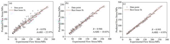
Figure 11.
Correlation between the predicted and experimental flow stress values from: (a) Johnson–Cook model; (b) Modified Johnson–Cook model; (c) Strain-compensated Arrhenius model.
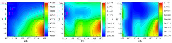
Figure 12.
Comparison of the AARE for: (a) Johnson–Cook model; (b) Modified Johnson–Cook model; (c) Strain-compensated Arrhenius model.
3.6. Thermal Processing Map
The thermal processing map can reflect the material instability zone and the distribution of the power dissipation factor under different thermal deformation parameters, and it can simply and intuitively guide the thermal processing technology [21]. In order to better optimize the hot working process parameters, the thermal processing map of Q345 steel is drawn.
The total power P obtained from the outside during the deformation process of the alloy material is the power consumed during the plastic deformation of the material (G) and the power consumed by the evolution of the material structure (J). It can be seen that the greater the J/P value, the more input power for plastic transformation of material structure, the higher the degree of plastic improvement recovery recrystallization of structure, and the better the thermal workability of the material.
The plastic strain rate sensitivity factor m is used to describe the relationship between the external plastic deformation power consumption and the internal tissue transformation power consumption. The expression is:
If the material is in the ideal linear dissipation state, the dissipation parameter m = 1, which means that the Q345 experimental steel is already in the ideal linear dissipation process, and J takes the maximum value. At this time,.
However, in the actual process, J cannot be maximized, and the ratio of energy consumption to the maximum linear dissipated energy is taken as the dissipation factor η of material power:
According to the power dissipation efficiency η under different conditions, a three-dimensional distribution diagram of η with the deformation temperature, strain rate, and strain was constructed as shown in Figure 13a. It can be found that η increases as the amount of deformation increases.
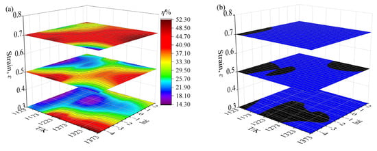
Figure 13.
(a) Power dissipation maps of Q345 under the different strain; (b) Instability diagram of Q345 under the different strain.
According to the dissipation rate Equation (22) given by Ziegler, the three-dimensional distribution diagram of ξ with the deformation temperature, strain rate, and strain change is shown in Figure 13b.
is the instability parameter of the material, which usually changes with the change of deformation temperature and deformation rate. If is negative, it indicates that the material is in an unstable state under the deformation condition, where blue is the stable region and black is the unstable region.
From Figure 13a,b, the thermal processing map of Q345 steel can be obtained:
The shaded area in Figure 14 is the flow instability zone that may occur during the thermal compression deformation of Q345 steel, and the instability zone is negative. It is well-noticed from the thermal processing map that when the strain temperature of Q345 steel is 1123–1373 K and the strain rate is 0.01–10 , the high dissipation value on the isoline is concentrated at the temperature of 1273–1248 K, and the strain rate is 0.01–0.05 . Considering that softening (dynamic recovery and dynamic recrystallization) is a common occurrence in this area, the thermal processing performance is relatively positive. In the low strain rate zone, Q345 steel is in the temperature intervals 1123–1153 K and 1198–1353 K; the processing interval of the strain rate 0.01–0.4 is the rheological instability zone; the distribution area is larger; and the high strain rate is only at the temperature 1123–1148 K. The instability occurs in the processing interval of strain rate 0.01–0.4 . This may be due to the low deformation energy provided by the low strain rate, limiting the occurrence of recrystallization. In this case, twins, shear, or microscopic textures are prone to occur, and the material properties are unstable. Comprehensively, the best processing interval should be: temperature 1253–1373 K, strain rate 0.5–10 [22,23].
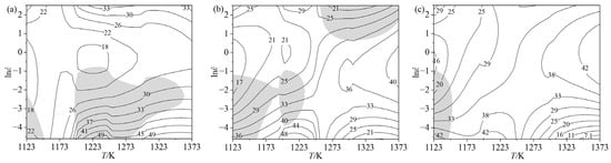
Figure 14.
Thermal processing maps of Q345 under the different strains: (a) ɛ = 0.3; (b) ɛ = 0.5; (c) ɛ = 0.7.
4. Conclusions
The hot deformation behavior of Q345 steel was investigated under the strain temperatures of 1123, 1173, 1223, 1273, 1323, and 1373 K and the strain rates of 0.01, 0.1, 1, and 10 through the thermal compression experiment. Based on the experimental true stress–true strain data, the Johnson–Cook model, the Modified Johnson–Cook model, the Strain-compensated Arrhenius constitutive model, and the thermal processing map of Q345 steel were constructed. The accuracy and efficacy of the three models in predicting the high temperature flow stress was compared and studied. According to the research results, the following conclusions can be drawn:
- The correlation coefficients (R) of the Johnson–Cook model, the Modified Johnson–Cook model, and the Strain-compensated Arrhenius constitutive model are 0.96537, 0.98844, and 0.99464, respectively. The average relative errors (AARE) are 25.0669%, 10.0032%, and 4.9339%, respectively. In contrast, the accuracy of the strain-compensated Arrhenius model is higher.
- The three constitutive models all have certain errors and show certain changes with the increase of temperature and strain rate. The main reason may be that the deformation of Q345 steel at higher temperatures and strain rates is highly nonlinear.
- The instability area of Q345 steel is mainly distributed at low temperature and low strain rate. However, the dissipation value is large in the strain temperature 1253–1373 K and strain rate 0.5–10 s−1, which means that the material is prone to dynamic recrystallization. At this time, the material has stable properties and good processing properties.
Author Contributions
Conceptualization, G.Z. and H.L.; methodology, G.Z. and Y.T.; formal analysis, G.Z.; investigation, Y.T., Y.S. and J.Z.; resources, G.Z; data curation, Y.T. and Y.S.; writing—original draft preparation, Y.T.; writing—review and editing, G.Z., Y.T. and J.L.; visualization, J.L.; supervision, G.Z. and H.L.; funding acquisition, G.Z., J.L. and H.L. All authors have read and agreed to the published version of the manuscript.
Funding
This research was funded by the National Key Research and Development Program of China (2018YFA0707305); the Scientific and Technological Innovation Programs of Higher Education Institutions in Shanxi (2021L292), Fundamental Research Program of Shanxi Province (20210302124009 and 20210302123207) and Taiyuan University of Science and Technology Scientific Research Initial Funding (20212026).
Institutional Review Board Statement
Not applicable.
Informed Consent Statement
Not applicable.
Data Availability Statement
Not applicable.
Acknowledgments
The authors would like to thank the Provincial Special Fund for Coordinative Innovation Center of Taiyuan Heavy Machinery Equipment for providing the facilities for the experimental works.
Conflicts of Interest
The authors declare no conflic of interest.
References
- Zhang, C.T.; Wang, R.H.; Zhu, L. Mechanical properties of Q345 structural steel after artificial cooling from elevated temperatures. J. Constr. Steel Res. 2021, 176, 106432. [Google Scholar] [CrossRef]
- Zhao, Z.W.; Zhang, H.W.; Xian, L.N.; Liu, H.Q. Tensile strength of Q345 steel with random pitting corrosion based on numerical analysis. Thin-Walled Struct. 2020, 148, 106579. [Google Scholar] [CrossRef]
- Schino, A.D.; Testani, C. Corrosion behavior and mechanical properties of AISI 316 stainless steel clad Q235 plate. J. Metals. 2020, 10, 552. [Google Scholar] [CrossRef]
- Schino, A.D. Analysis of phase transformation in high strength low alloyed steels. Metalurgija 2017, 56, 349–352. [Google Scholar]
- Chen, W.; Ye, J.H.; Jin, L.; Jiang, J.; Liu, K.; Zhang, M.; Chen, W.W.; Zhang, H. High-temperature material degradation of Q345 cold-formed steel during full-range compartment fires. J. Constr. Steel Res. 2020, 175, 106366. [Google Scholar] [CrossRef]
- Guo, Y.B.; Fang, C.; Zheng, Y. Post-fire hysteretic and low-cycle fatigue behaviors of Q345 carbon steel. J. Constr. Steel Res. 2021, 187, 106991. [Google Scholar] [CrossRef]
- Johnson, G.R.; Cook, W.H. Fracture characteristics of three metals subjected to various strains, strain rates, temperatures and pressures. Eng. Fract. Mech. 1985, 21, 31–48. [Google Scholar] [CrossRef]
- Sellars, C.M.; McTegart, W.J. On the mechanism of hot deformation. Acta Metall. 1966, 14, 1136–1138. [Google Scholar] [CrossRef]
- Song, Y.H.; Wang, S.; Zhao, G.H.; Li, Y.G.; Li, J.; Zhang, J. Hot deformation behavior and microstructural evolution of 2205 duplex stainless steel. Mater. Res. Express. 2020, 7, 046510. [Google Scholar] [CrossRef]
- Sahu, S.; Mondal, D.P.; Goel, M.D.; Ansari, M.Z. Finite element analysis of AA1100 elasto-plastic behaviour using Johnson-Cook model. Mater. Today. Proc. 2018, 5, 5349–5353. [Google Scholar] [CrossRef]
- Bobbili, R.; Madhu, V. A modified Johnson-Cook model for FeCoNiCr high entropy alloy over a wide range of strain rates. Mater. Lett. 2018, 218, 103–105. [Google Scholar] [CrossRef]
- Yang, X.W.; Wang, Y.Y.; Dong, X.R.; Peng, C.; Ji, B.J.; Xu, Y.X.; Li, W.Y. Hot deformation behavior and microstructure evolution of the laser solid formed TC4 titanium alloy. Chin. J. Aeronaut. 2021, 34, 163–182. [Google Scholar] [CrossRef]
- Lin, X.J.; Huang, H.J.; Yuan, X.G.; Wang, Y.X.; Zheng, B.W.; Zuo, X.J.; Zhou, G. Establishment and validity verification of the thermal processing map of a Ti-47.5Al-2.5V-1.0Cr-0.2Zr alloy with a lamellar microstructure. Mater. Charact. 2022, 183, 111599. [Google Scholar] [CrossRef]
- Song, Y.H.; Li, Y.G.; Zhao, G.H.; Liu, H.T.; Li, H.Y.; Li, J.; Liu, E.Q. Electron Backscatter Diffraction Investigation of Heat Deformation Behavior of 2205 Duplex Stainless Steel. Steel Res. Int. 2021, 92, 2000587. [Google Scholar] [CrossRef]
- Chao, Z.L.; Jiang, L.T.; Chen, G.Q.; Zhang, Q.; Zhang, N.B.; Zhao, Q.Q.; Pang, B.J.; Wu, G.H. A modified Johnson-Cook model with damage degradation for B4Cp/Al composites. Compos. Struct. 2021, 282, 115029. [Google Scholar] [CrossRef]
- Lin, Y.C.; Chen, X.M.; Liu, G. A modified Johnson—Cook model for tensile behaviors of typical high-strength alloy steel. Mater. Sci. Eng. A 2010, 527, 6980–6986. [Google Scholar] [CrossRef]
- Wang, Y.T.; Zeng, X.G.; Chen, H.Y.; Yang, X.; Wang, F.; Zeng, L.X. Modified Johnson-Cook constitutive model of metallic materials under a wide range of temperatures and strain rates. Results Phys. 2021, 27, 104498. [Google Scholar] [CrossRef]
- Li, J.; Zhao, G.H.; Chen, H.Q.; Huang, Q.X.; Ma, L.F.; Zhang, W. Hot deformation behavior and microstructural evolution of as-cast 304L antibacterial austenitic stainless steel. Mater. Res. Express. 2018, 5, 025405. [Google Scholar] [CrossRef]
- Li, J.; Zhao, G.H.; Ma, L.F.; Chen, H.Q.; Li, H.Y.; Huang, Q.X.; Zhang, W. Hot Deformation Behavior and Microstructural Evolution of Antibacterial Austenitic Stainless Steel Containing 3.60% Cu. J. Mater. Eng. Perform. 2018, 27, 1847–1853. [Google Scholar] [CrossRef]
- Rezaei Ashtiani, H.R.; Shayanpoor, A.A. Prediction of the Hot flow Behavior of AA1070 Aluminum Using the Phenomenological and Physically-Based Models. Phys. Met. Metall. 2021, 122, 1436–1445. [Google Scholar] [CrossRef]
- Lu, J.; Song, Y.L.; Hua, L.; Zheng, K.L.; Dai, D.G. Thermal deformation behavior and processing maps of 7075 aluminum alloy sheet based on isothermal uniaxial tensile tests. J. Alloy. Compd. 2018, 767, 856–869. [Google Scholar] [CrossRef]
- Ye, L.Y.; Zhai, Y.W.; Zhou, L.Y.; Wang, H.Z.; Jiang, P. The hot deformation behavior and 3D processing maps of 25Cr2Ni4MoV steel for a super-large nuclear-power rotor. J. Manuf. Processes. 2020, 59, 535–544. [Google Scholar] [CrossRef]
- Kumar, S.; Karmakar, A.; Nath, S.K. Construction of hot deformation processing maps for 9Cr-1Mo steel through conventional and ANN approach. Mater. Today Commun. 2021, 26, 101903. [Google Scholar] [CrossRef]
Publisher’s Note: MDPI stays neutral with regard to jurisdictional claims in published maps and institutional affiliations. |
© 2022 by the authors. Licensee MDPI, Basel, Switzerland. This article is an open access article distributed under the terms and conditions of the Creative Commons Attribution (CC BY) license (https://creativecommons.org/licenses/by/4.0/).