The Development and Verification of a Simulation Model of Shape-Memory Alloy Wires for Strain Prediction

Abstract

One of the greatest challenges in the design of shape-memory elements (mostly binary Nickel-Titanium wires) is to ensure that the required travel (stroke) is achieved, as this is subject to variation due to various influencing factors. One way of predicting the stroke is to use a suitable energy model. In the past, for example, a model was developed by Oelschläger with which the stroke can be calculated on the basis of the electrical energy. However, so far no model takes into account the change of the phase transformation temperature. In this study, the model of Oelschläger is extended and verified to consider the degradation behavior over the whole lifetime. For this purpose, fatigue tests of 52 wires (2 different load scenarios) were performed. Based on these tests and the application of statistical methods (distribution models, goodnes-of-fit tests etc.), a target model was developed for each load scenario, which is used to verify the extended energy model. The energy model was applied to wires of both load scenarios to simulate the stroke progression. The verification of the extended simulation model shows that it is possible to simulate the longterm behavior of the stroke for one of the two load scenarios. The second load scenario shows deviations between the target model and the simulation, which is due to problems in the area of measurement equipment, convection, and temperature distribution in the wire. Nevertheless, a decisive modeling approach could be developed, which can be used to consider the long-term behavior of the phase transformation temperature of wires in simulations.

1. Introduction

Shape Memory Alloys (SMA) have the fascinating ability to regain their original shape after an apparent plastic deformation [1,2,3,4]. This is due to a diffusionless phase transformation between a low temperature phase martensite and a high temperature phase austenite [2]. This transformation process leads to the deformation of the material that is most commonly used to generate a stroke [5]. This effect makes SMAs very suitable for actuator designs in which they substitute for conventional actuator elements, such as electric engines [6]. SMA components, such as wires, springs or tubes, are lightweight, small, noiseless during operation and have a high energy to density ratio [7]. There are two different Shape Memory Effects (SME): pseudoplasticity (or thermal SME) and pseudoelasticy (or mechanical SME) [8]. In actuator designs the thermal SME is used. The SMA component is heated via the ambient medium [9] or via electric heating [10]. The activation temperature depends on the specific SM Alloy and the applied stress [5]. Over the last decades SMAs reached various fields of applications, such as automotive [11], aviation [12,13,14,15], medicine [16,17,18], robotics especially micro and soft robotics [19,20,21,22,23]. Over the last decade additive manufacturing became a relevant process to fabricate NiTi [24,25]. The interest in the process to generate superelastic structures is of great interest in recent research [26,27,28]. Another advantage that makes SMAs so attractive is their so called integrated sensing effect [6,7]. It is applied when the SMA component is electrically heated since the electric resistance is changed during the phase transformation. Figure 1 shows the course of the resistance changes over time. Monitoring the resistance during operation allows to make statements about the components condition [29] since the contraction and the elongation of the SMA component is accompanied with a change in the electrical resistance. Unfortunately there are several fatigue effects that limit the accuracy of these methods.

Shown in Figure 1 are the courses of the stroke (Left) and the maximum of the electric resistance per stroke (Right) at different load scenarios until failure. Two effects are obvious:

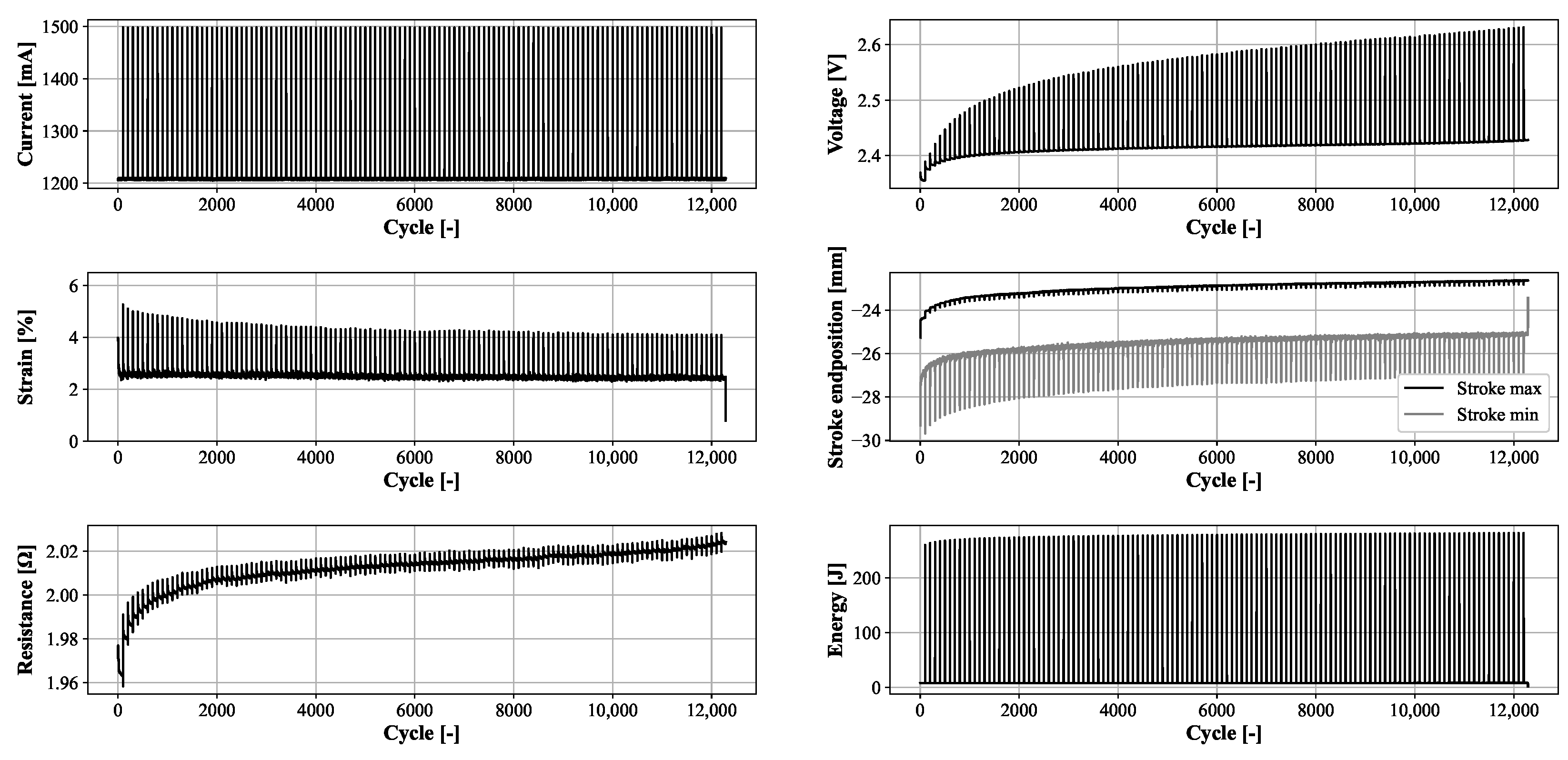
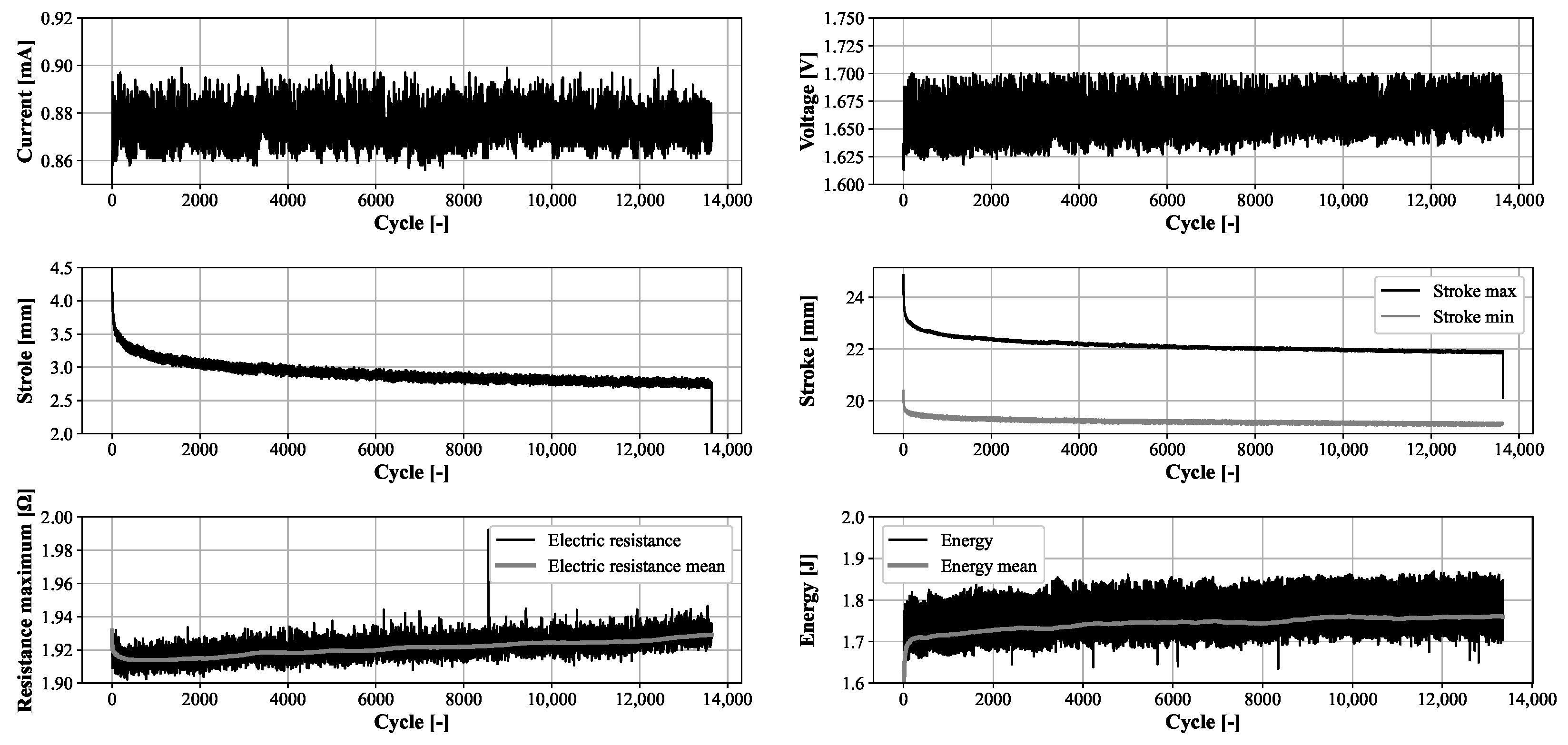
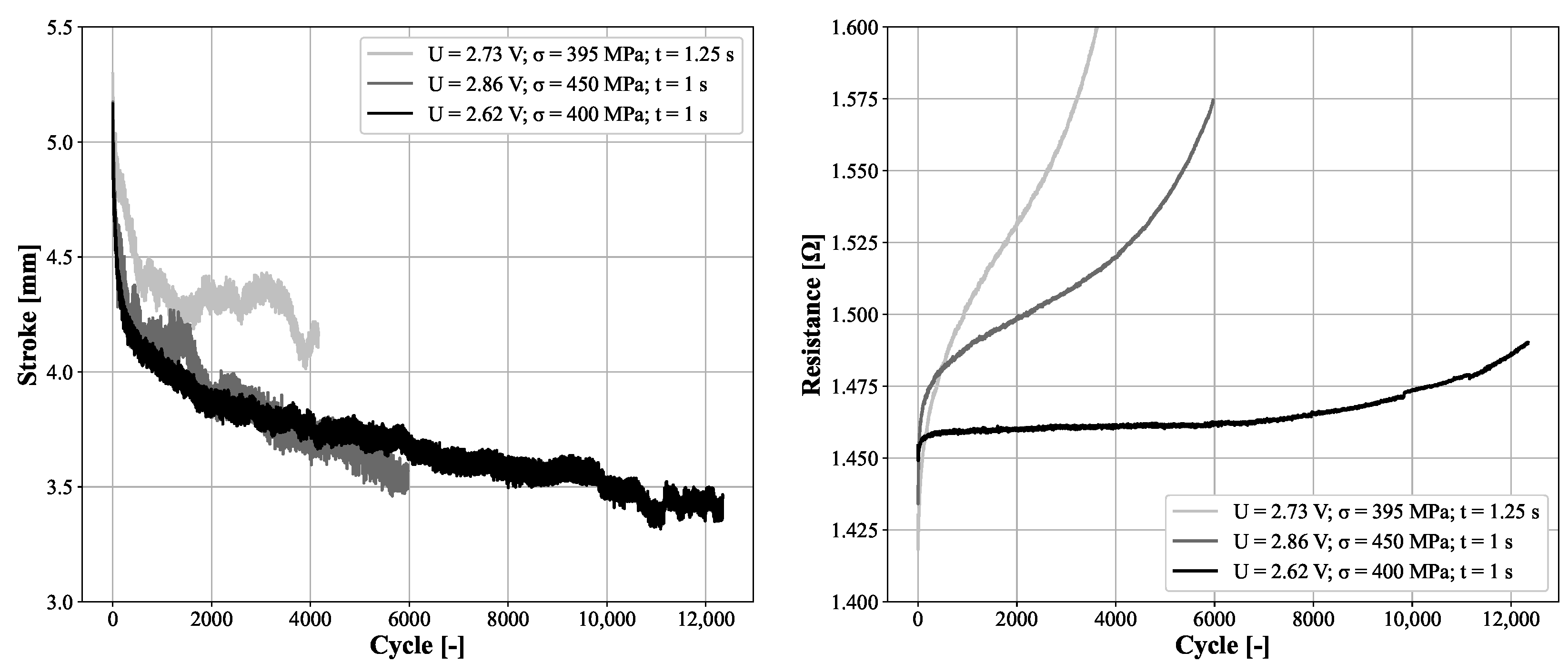
• The maximum stroke decreases over time different. The process depends on the load scenario.
• The electric resistance increases over time. It also depends on the load scenario.

The exact connection between fatigue, load, and resistance is yet to be described. This degradation makes it complicated for a resistance-based condition monitoring to work properly over the complete lifecycle of an SMA component. Within the scope of several publications, Heß and Bracke developed different approaches to predict the (remaining) lifetime of shape memory wires [31,32,33,34,35]. For example, the influence of temperature due to weather and various load scenarios were investigated. For the analyses, fatigue tests were carried out, as in this work, and then evaluated using various statistical procedures and methods (nonparametric statistics, correlation analysis, regression analysis etc.). Prediction models were developed on the basis of the parameters stroke (and the integral of the stroke), electrical voltage, current intensity and electrical resistance, and are currently being further developed. Acceleration factors were also determined for the load parameters weight and current intensity.

Fatigue of SMAs can be divided in two major areas: structural and functional fatigue. Structural fatigue is described as the formation and growth of cracks during cyclic, mechanic load of the material [36,37]. This effect is well investigated for pseudoelastic SMA. From this field it is known, that the lifetime (number of cycle until crack) is driven by the initiation of cracks [38,39,40]. Functional fatigue is more complex. The martensitic phase transformation is known as reversible but is guarded by irreversible processes on the micro- and nano scale [41]. This leads to decreasing austenite start temperatures and increasing austenite finish temperatures with rising activation cycles [42]. Both effects lead to an increase of the electric resistance over time. Figure 2 shows the stroke/temperature hysteresis at different activation cycles. The shown activation cycles were performed in the climate chamber. The cycles between the climate chamber cycles were electrically induced. A binary NiTi wire with a diameter of 0.28 mm was investigated at a load of 350 MPa. According to the work of Großmann the phase transformation temperature changes with an increasing number of activation cycles [42]. These change strongly depending on the load scenario.

The first cycle shows a very sharp austenite start and finish temperature: Between about 125 °C and 127 ° C the full stroke of 5 mm (Figure 2 Mid) is generated. The same is true for martensite start ($M_S$) and finish ($M_F$) temperature. Starting after the first activation an elongation of the wire can be observed: After cooling the wire does not go back to the initial position but goes a bit further. During the following cycles the hysteresis diffuses gradually in an increasing manner since the temperature range of the transformation widens. The shown PTT are used later on for the simulation.

2. Goal of Research Work/Motivation

The simulation of the SME is of great interest for the scientific community for more than two decades [43,44,45,46]. The research is mainly focused on the stress-induced martensitic transormation or superelasticity of SMA. The role of the transformation temperature became a topic later on and is still subject for researchers [47,48]. Still, the influence of the fatigue over the whole lifespan of an SMA component on the applicability of the mentioned approaches is not yet known.

One major goal to achieve by monitoring the electrical resistance is the position control of the SMA component. There are two ways to investigate this: How can the position of an SMA component be controlled during operation? How can the generated stroke based on an SMA component be estimated based on certain activation parameters while designing an SMA actuator? There are several solutions for the first question: Schiedeck and Elahinia used a PI or a PID controller in order to control the position of SMA wires based on either the electric resistance or the stroke signal of a distance sensor [10,49]. Elahinia went further [50] and investigated several more control mechanisms for this topic. Pagel finally developed a control system that is able to set a certain position independent from the load scenario by applying a thermal low pass characteristic [51,52].

$$\begin{array}{ll}\underset{\begin{array}{c}Electr.power\end{array}}{\underbrace{I^2\left(t\right)·R_D}}=& \underset{\begin{array}{c}Thermalcapacity\end{array}}{\underbrace{C_p·p·V_D·\frac{d{T}_D}{dt}}}+\underset{\begin{array}{c}Convectiveheattransfer\end{array}}{\underbrace{\alpha ·F_D·(T_D-T_U)}}+\underset{\begin{array}{c}Heattransferbyradiation\end{array}}{\underbrace{{\mathcal{E}}_m·{\sigma }_S·F_D·({T_D}^4-{T_U}^4)}}+\\ & \underset{\begin{array}{c}\mathit{Transformation} \mathit{enthalpy}\end{array}}{\underbrace{p·V_D·\Delta H·\left|\frac{d\xi }{dt}\right|}}+\underset{\begin{array}{c}\mathit{mech}.power\end{array}}{\underbrace{\frac{{\mathit{dW}}_{\mathit{Mech}}}{dt}}}\end{array}$$

(1)

For the second question Oelschläger developed an approach based on the energy balance: Electric energy goes into the component and heat content, convection, radiation, work (by lifting a weight) and phase transformation enthalpy leaves the component (see Equation (1)). The heat conduction is neglected, since its magnitudes are smaller than convection and radiation [53,54]. Since then this approach was used several times and for various applications [55,56,57,58,59].

$$A_s\le T_D\le A_f:\xi =\frac{\xi }{2}cos\left(\pi \frac{T_D-A_s}{A_f-A_s}\right)+\frac{\xi }{2}$$

(2)

To calculate the strain of the SMA component and the resulting stroke Equation (3) is used. The formula goes back to an approach by Liang and Rogers [60]. Depending on the phase transformation temperatures $A_S$ and $A_F$ the amount of martensite ($\xi$) is calculated for a certain temperature of the component. From there on the strain respectively the stroke is calculated as followed:

$${\mathcal{E}}_{FG}={\mathcal{E}}_{FG,max}(1-\xi )$$

(3)

For the Equation to calculate correct values the initial parameters must be known. With a deeper look into Equation (1) these parameters are: The mass of the component respectively its outer dimensions and its density and the phase transformation temperature. The components’ mass is important for the heat content. The convection and the radiation depend on the components surface. The phase transformation enthalpy strongly depends on exact values of the materials phase transformation temperatures. These can either be determined by DSC-measurements or in a climate chamber [61]. Finally the maximum strain that also decreases over time must be determined and taken into account.

Figure 3 and Figure 4 clearly show that all values change with an increasing number of activation cycles and moreover depend on the load scenario and the specific alloy. In this expirement, a 100 mm long binary NiTi actuator wire with a diameter of 0.28 mm was loaded with 350 MPa. It was electrically activated with 1.2 A for 3 s followed by a cool down phase of 40 s. This resulted in a strain of approximately 3% or 3 mm. To monitor the decrease of the maximum strain every hundredths cycle the specimen was fully activated like this: A slow electric ramp starting at 0 A and linearly increasing the current of 1.5 A in 100 s followed by a ramp down back to 0 A in 100 s. An example of this effect is shown in Figure 3. All these uncertainties make it a challenge to properly predict or simulate the strain respectively the stroke of an SMA component.

Summary and leading question: Controlling the stroke of an SMA component is a major goal to achieve. A literature review showed that several approaches were investigated to determine the stroke. None of the approaches take the change of the phase transformation temperature into account. Various experiments found a link between the fatigue of an SMA component and its electric resistance. Therefore the main question of this study is: Can the electric resistance be used in order to adjust the PTT during the operation of an SMA component? Can the resulting stroke for higher cycle counts still be calculated with values for the PTT that were adjusted according to the electric resistance? How reliable does a developed model that predicts the stroke perform?

3. Experimental Setups

The development of the adapted model for the prediction of the actuator travel requires numerous fatigue tests and calibration tests, some of them within a climatic chamber. The strain development of the reference model also requires an extensive data base in the form of fatigue tests. This chapter therefore describes in detail the test setups used (test benches, test plans, etc.), the execution of the tests, and the measurement data and parameters generated in the process. The description of Section 3.1 is based on [30,31,33,35], the description of Section 3.2 is based on [30,62].

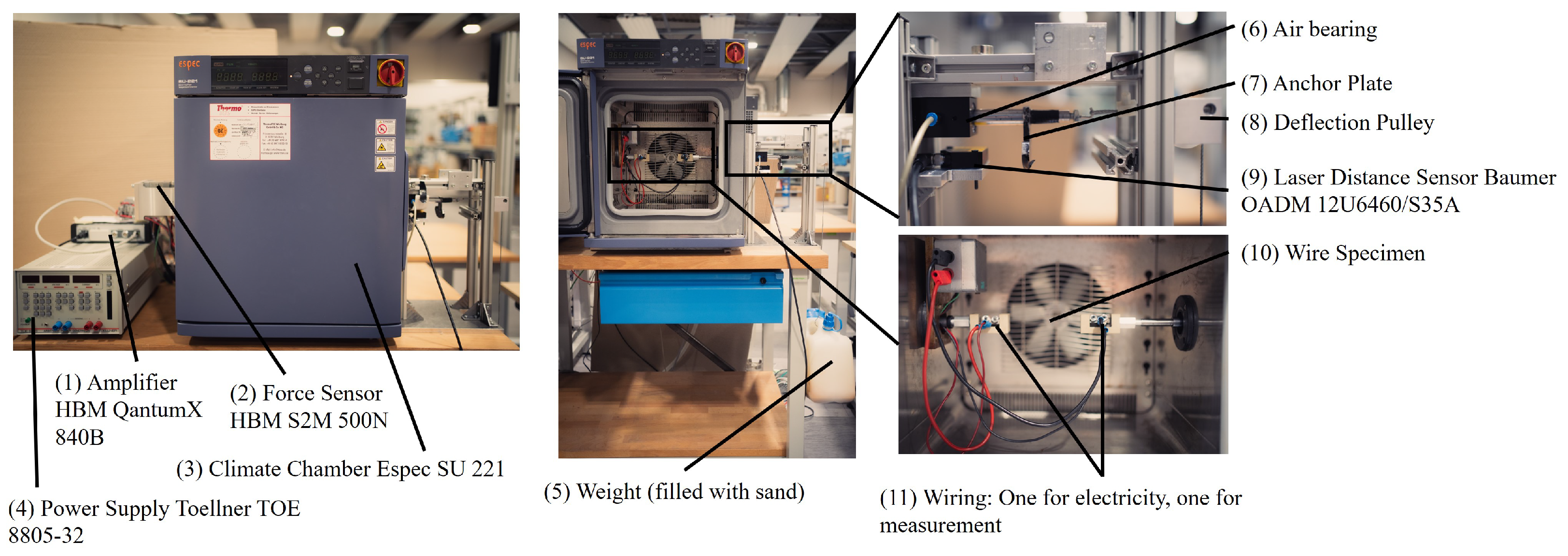
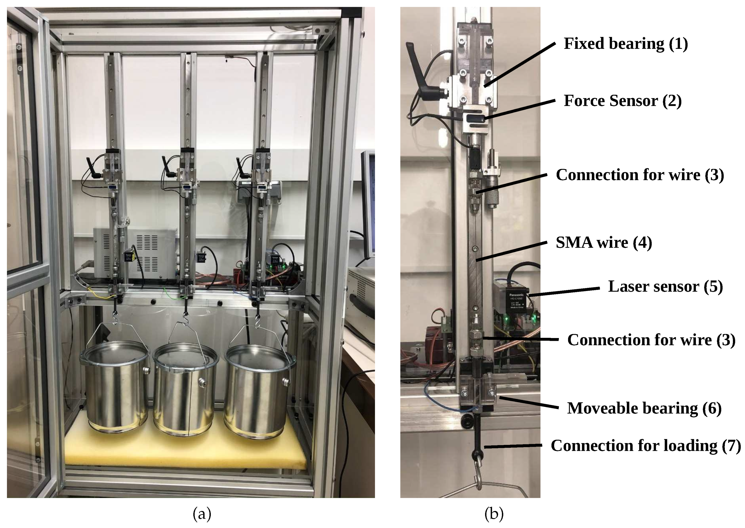
3.1. Experimental Setup for Fatigue Tests

The test rig in Figure 5 is designed for parallel fatigue testing of three SMA wires. Figure 5a shows the whole test rig consisting of 3 test channels, Figure 5b shows the components of one test channel in detail. All SMA wires (4) are cut to the same length of about 110 mm and connected (3) to a fixed bearing (1) and a moveable bearing (6) which have a defined displacement to each other. During the experiments the resulting length of the wires is thus 90 mm which is standardized by the VDI-guideline 2248 [63]. Defined loadings are attached to a connection of the moveable bearing (7). The weight is lifted by the wire during the tests and serves also as the resetting element during the cooling phase. Before the test procedure, the upper fixed bearing (1) is loosened and moved upward to pretension the wire. In this case, the weight is already mounted. Every wire has the same pretension based on the applied loading. Subsequently, the fixed bearing is fixed again (with a screw). The wires are connected to a power source, every test channel consists also of a force sensor (2) and a laser displacement sensor (5). Additionally, the test rig also has a temperature sensor in its housing measuring the ambient temperature inside the test rig.

During the entire course of the fatigue tests, all wires are cyclically heated above the austenite starting temperature $A_S$ with defined parameters and thus activated. Important parameters are among others the electrical voltage [V] and current [A] for activation, the mechanical loading [MPa], the activation duration [s], the cooling phase duration [s], the ambient temperature [℃], the force [N] and the displacement [mm]. Different wire diameters d and loadings m can be compared by relating the loading to the wire cross-section, i.e., by calculating the mechanical stres $\sigma$ using the Equation (4).

$$\sigma =\frac{mg}{{\left(\frac{d}{2}\right)}^2\pi }$$

(4)

An example of 1 cycle of a measurement series of the endurance test rig is shown in Figure 6. Exemplary the measured quantities distance, force and electrical voltage are plotted against time. It can be clearly seen that the shape memory effect is caused by the current pulse at a voltage of about 1.7 V. The wire immediately lifts the weight, which is measured by the distance sensor as displacement. In the example shown the maximum displacement is approx. 3.2 mm and is already reached after about 1 s. On the other hand, the cooling phase takes about 12 s. During the cooling phase, the weight elongates the wire again and acts as the reset element so that the next activation can start immediately following the previous cycle. This is a simple setup for accelerated testing [64,65,66,67]. The force sensor does not measure the generated positioning force, it measures the changes in the weight force. This allows, for example, to observe whether activations that are too fast lead to oscillatory behavior, that causes additional damage.

Following the experiments, all maximum, minimum values and the delta of all process parameters are determined for each individual loading cycle, so that the behavior of each parameter can be visualized over the entire test time. Figure 7 shows the corresponding curves for an experiment as an example. The curves of various process parameters over the entire test period can be seen. For example, the degradation of the actuator travel over the load cycles becomes clear, while the resistance increases and thus also more electrical voltage is required.

After the extraction of all peak values, data cleaning is performed to eliminate large outliers, which is necessary for accurate evaluations. The measured data is smoothed with a Hampel filter by Pearson [68], which is defined in Equation (5). The filter identifies outliers in time series using the parameter threshold t and and a window size for the calculation. The lower the threshold, the more points are declared as outliers. The minimum threshold is 0 while the highest is 3. In order to eliminate only large outliers and to influence the data sets as little as possible, a threshold of 3 is used, as well as a window size of 100 cycles.

$$y_k=\left\{\begin{array}{c}{x}_k|x_k-x_k^{†}|\le t{S}_k\hfill \\ x_k^{†}|x_k-x_k^{†}|>t{S}_k,\hfill \end{array}\right.$$

(5)

Within the scope of the paper, 2 series of experiments with different test setups I and $II$ are analyzed and used for the development of the models. Test setup I uses a load of 300 MPa, the wires are activated at 0.8 A for 3 s while the cooling phase lasts 40 s. Test setup $II$ uses a load of 350 MPa, the wires are activated at 2.7 Volts for 1 s while the cooling phase lasts 12 s. Due to the fact that both settings are very different from each other, two completely different load scenarios can be used for the analysis and model development. For all tests, the same heat-treated wire with an oxide layer and a diameter of 0.28 ± 0.01 mm as well as an austenite finish temperature $A_F$ of 85 ± 10 °C for the unloaded wire is used.

Table 1. Results of the fatigue tests performed: Cycles till failure of all tested wires for 2 different test setups.

Test Setup	Wire 1	Wire 2	Wire 3	Average
	10,389	5944	8258	8197
	14,395	13,135	6467	11,332
	13,014	11,502	5711	10,076
Test setup I	7997	11,967	7500	9155
Loading 350 MPa	14,127	12,055	6298	10,827
Current for activation 0.8 A	14,122	13,036	10,733	12,630
Activation 3 s	11,348	9282	9958	10,196
Cooldown time 40 s	15,425	13,722	11,859	13,669
	13,611	15,493	12,963	14,022
	16,222	12,478	13,780	14,160
	35,635	16,419	20,872	24,309
Test setup $II$	31,192	11,633	11,099	17,975
Loading 300 MPa	74,819	12,225	27,428	19,827
Voltage for activation 2.7 V	120,772	18,587	36,087	27,337
Activation 1 s	34,389	23,316	-	19,235
Cooldown time 12 s	70,127	22,117	-	22,117
	25,426	27,606	-	26,516

shows an overview of the load cycles to failure of all endurance tests performed. On average, the number of cycles to failure for test setup I is approx. 11,426. A maximum of 16,222 cycles was achieved, while the earliest point of failure was reached at 5711 cycles. In the setup $II$ tests, not all wires were tested to failure (gray values). These tests were aborted at different times. The aborted tests are not considered in the calculation of the average, but are used up to cycle 35,000 in the further course of the analysis and model development.

Furthermore, additional fatigue tests were performed with setup I using another test rig (Figure 8). This test rig is very similar to the previous test rig shown in Figure 5. The wire specimen (1) is clamped vertically between two clamping positions made of copper (2). When the wire is activated, the travel between a plate (3) and a fixed ultrasonic sensor (4) is measured. Weights (5) can be used to induce any desired mechanical voltage. Power supplies with arbitrary function (6) generate current waveforms that can be precisely regulated to control temperatures and temperature waveforms. Any sensor signals converge in a measuring amplifier (7) and are recorded on a measuring/control PC (8). The tests from this test bench are used as input variables for the simulations.

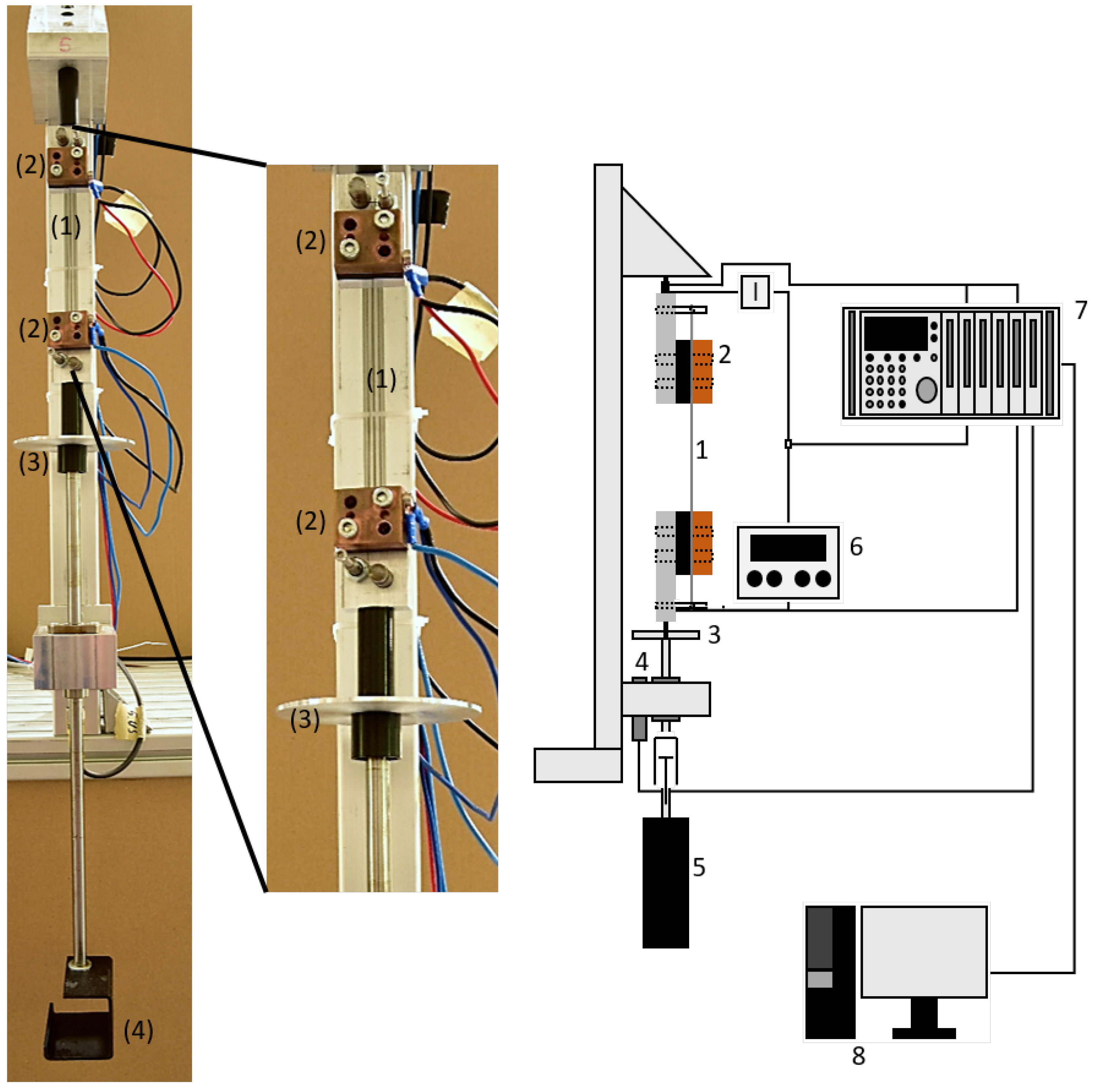
3.2. Experimental Setup for Climate Tests

Experimental setup $II$ is shown in Figure 9. It works similar to the first presented setup, with the main difference that all experiments can be performed within a climate chamber. This allows for either an electric activation at varying ambient temperatures, or an activation via the ambient temperature. Furthermore the power supply and the amplifier are of greater quality.

Table 2. Operation data of the power supply Toellner TOE-8805-32.

Power supply
Output voltage [V]	0–32
Output current [A]	0–5
Output power [W]	160
Rate of ascent/descent [V/$\mathsf{\mu }$s]	2
Output voltage
Resolution [mV]	2
Setting accuracy [mV]	0.025% + 10 mV
Measurement accuracy [mV]	0.1% + 10 mV
Output current
Resolution [mA]	5
Setting accuracy [mA]	0.1% + 80 mA
Measurement accuracy [mA]	0.1% + 80 mA

lists the operation data of the power supply. For a more detailed review of the test rig please see [62].

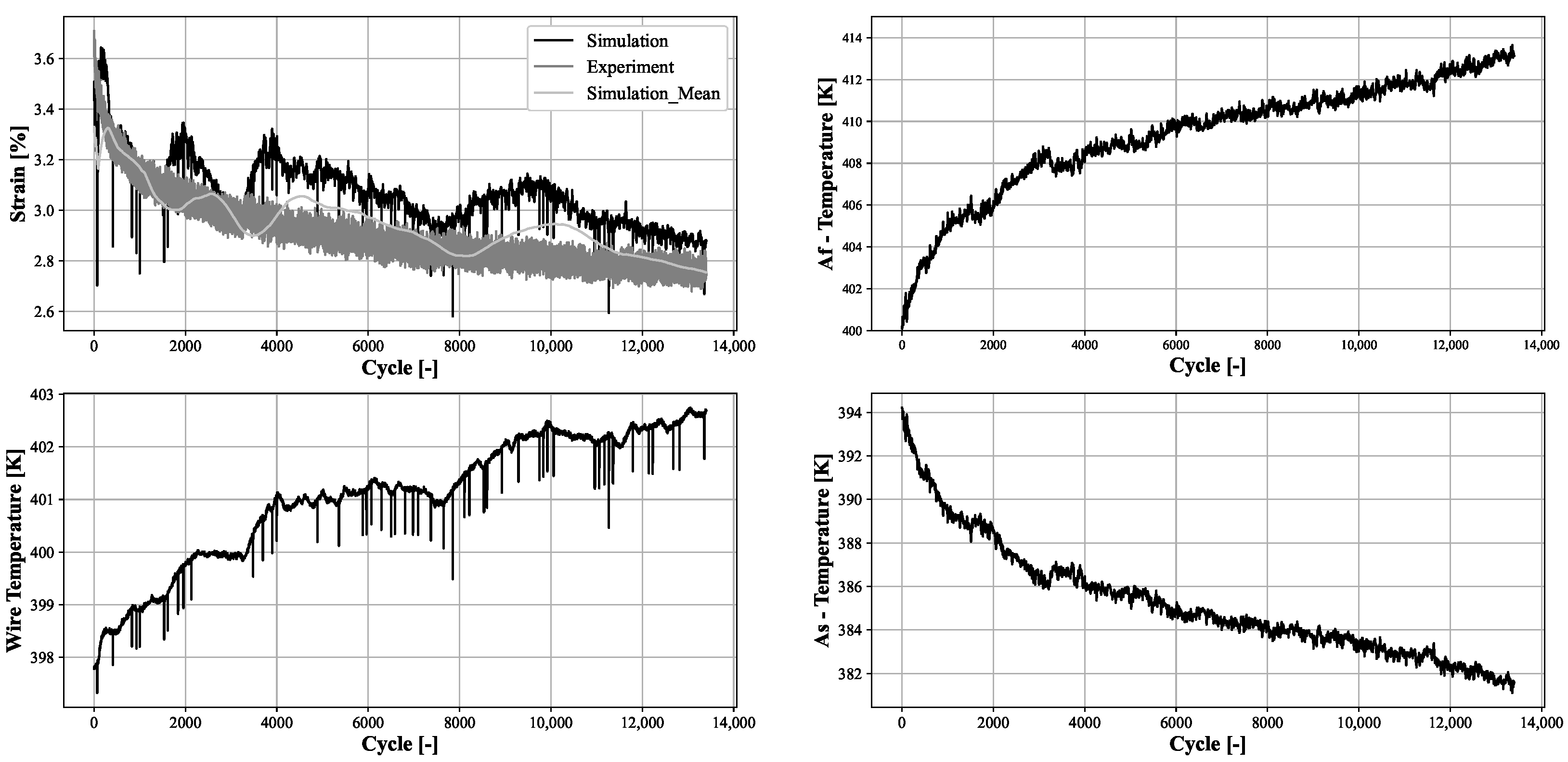
4. Model Setup of the Simulation and Plausibility Analysis

A model based on the approach of Oelschläger (see Section 2) was derived. The first order differential equation can be discretized for $\Delta T$ for a given time step by Equation (6):

$$\Delta T_d=\frac{\Delta Q_{elec}-\Delta Q_{conv}-\Delta Q_{rad}-\Delta Q_{trans}-W}{C_{P}P{V}_D}$$

(6)

For the given experimental setup the time step is equal to the measuring frequency (50 Hz or 20 Hz). For every time step Voltage and Current are measured. Thus the energy per time step is calculated by Equation (7):

$$\Delta Q_{elec}=IV\Delta t$$

(7)

From there on, the simulation calculates the resulting temperature difference for the given energy input and adds it to the previous value of wire temperature. At the end of each activation cycle $A_S$, $A_F$, maximum strain and the wire length (respectively the surface of the wire) are adjusted based on the change of the electric resistance. To prove that the simulation is running properly the plausibility was checked in detail. To start the analysis Figure 10 shows the stroke, the endpositions, the resistance, the current, the voltage and the energy each per cycle for the real experiment.

As expected the resulting stroke and the enpositions decrease with an increasing number of cycles. The current is controlled constant at approximately 880 mA. As mentioned before, the resistance increases over time. As a result the voltage increases as well. Since the energy is the product of voltage, current and the timestep it is increasing as well. Several assumptions are derived from the plots in Figure 10 going into the plausibility analysis:

• The predicted stroke decreases
• The maximum wire temperature increases since the energy increases
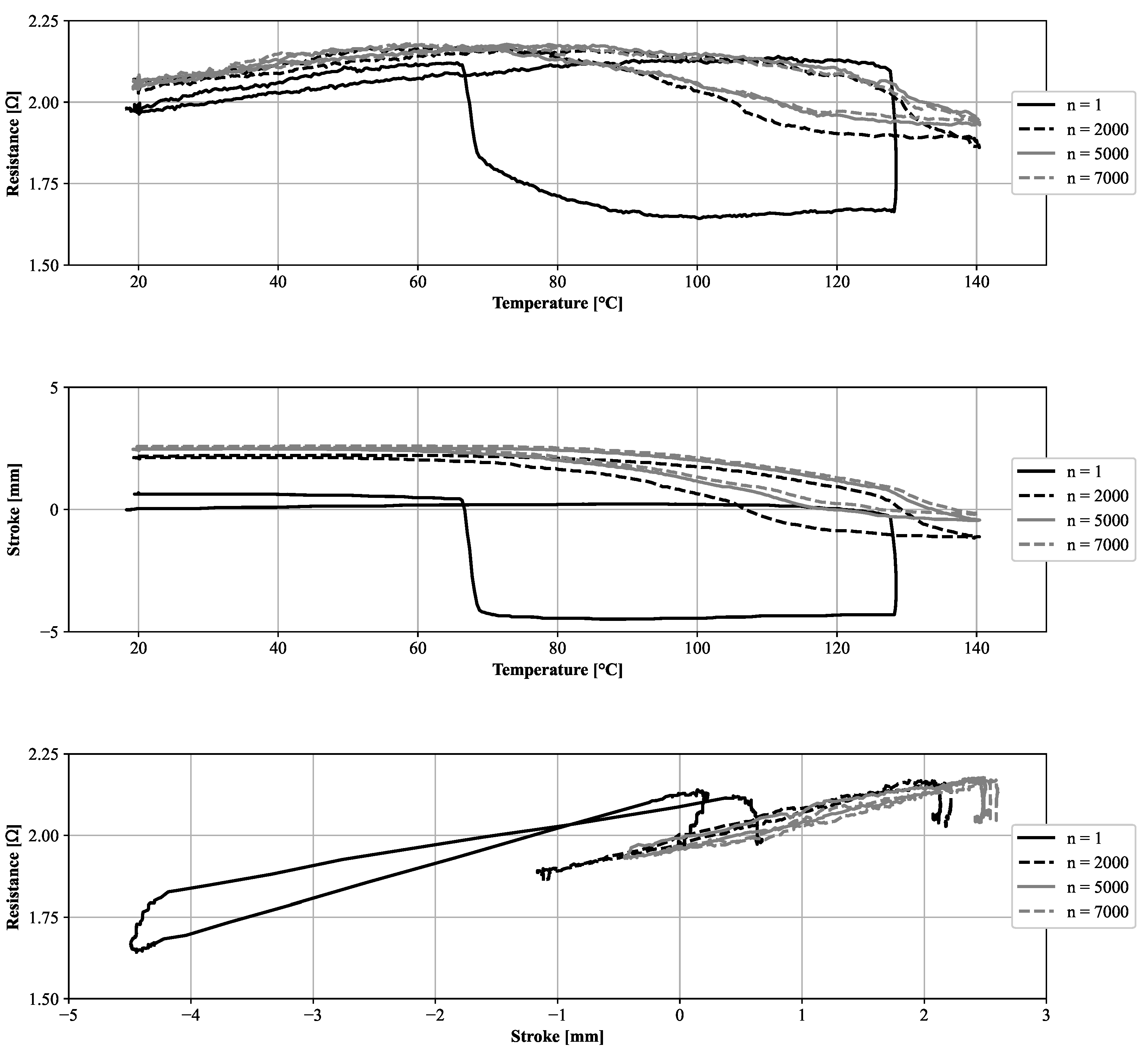
• $A_S$ should increase proportionally to the electric resistance
• $A_F$ should decrease proportionally to the electric resistance

To prove the assumptions, the simulated plot is shown in Figure 11.

The simulation was based on the input parameters for energy and electric resistance shown in Figure 10. Overall, the simulated stroke fits the measured values. A deeper statistical analysis of the predicted parameters is performed in Section 6. The assumption of a decreasing tendency in the stroke is met. At approximately cycle 1800, 3800 and 8000 the stroke starts to rise again. The reason for that lies in the accuracy of the measuring equipment. A further look into the electric resistance in Figure 10 shows the mean value of the electric resistance and the energy. Both variables behave accordingly: At the investigated cycles the resistance and the energy both show a “bump” that explains the deviation in the calculated stroke.

Forward, the calculated wire temperature must increase over time. This assumption is met. There are however still some outliers. The expectations for the course of $A_S$ and $A_F$ are met. Further on, the PTT of Figure 2 are met. The simulated temperatures align with the real temperatures from the experiment.

5. Development of the Target Models

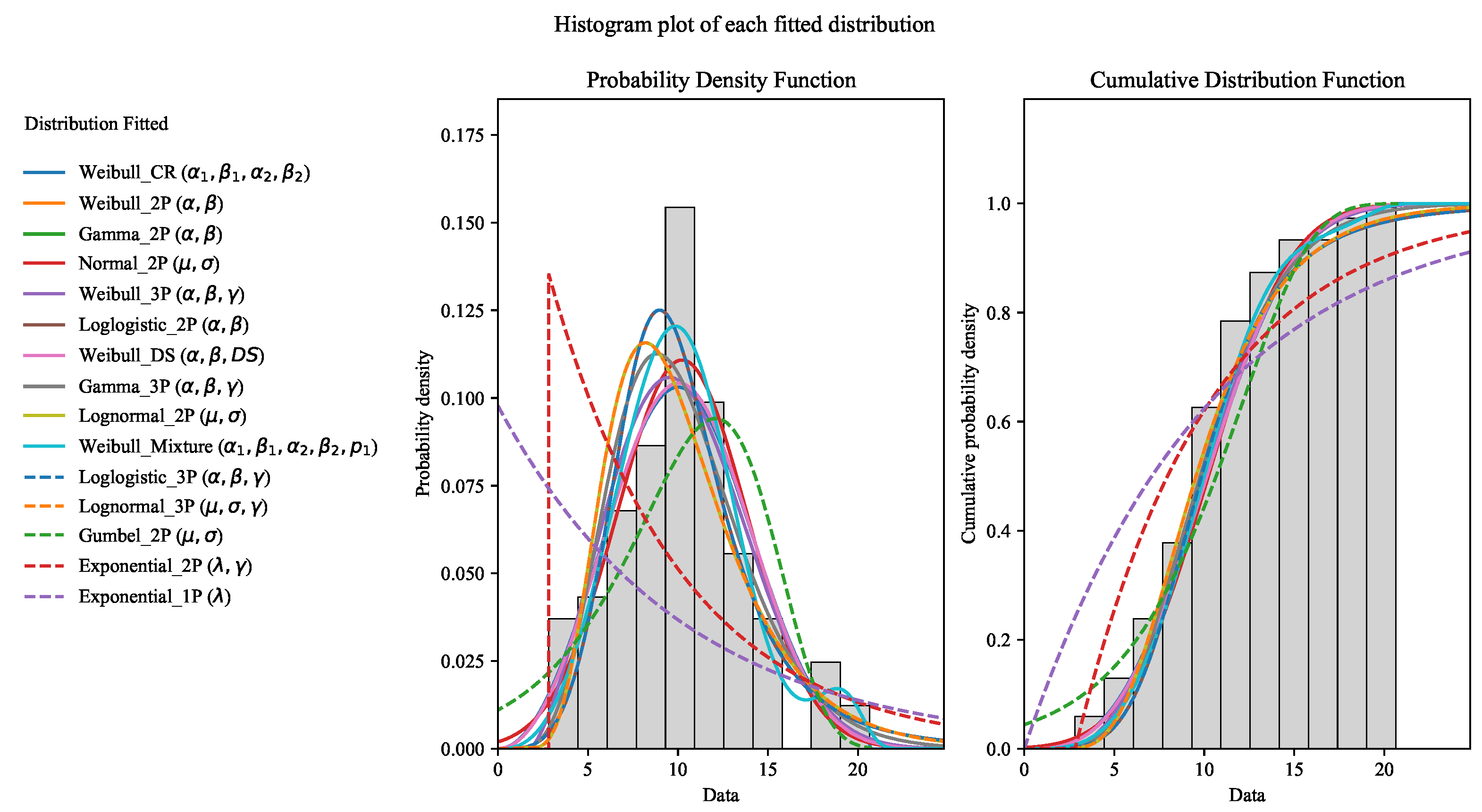
In this chapter, the statistical methods used for the development of the models are explained. These essentially include various distributions, the calculation of confidence intervals and different goodness-of-fit tests. In this chapter, some of the most commonly used distributions for reliability analysis [64,69,70,71,72,73,74] are described. A goodness-of-fit test (non-parametric hypothesis test) is used to test whether the data set (approximately) follows a certain distribution model. All relevant distribution models are explained below.

5.1. Distributions

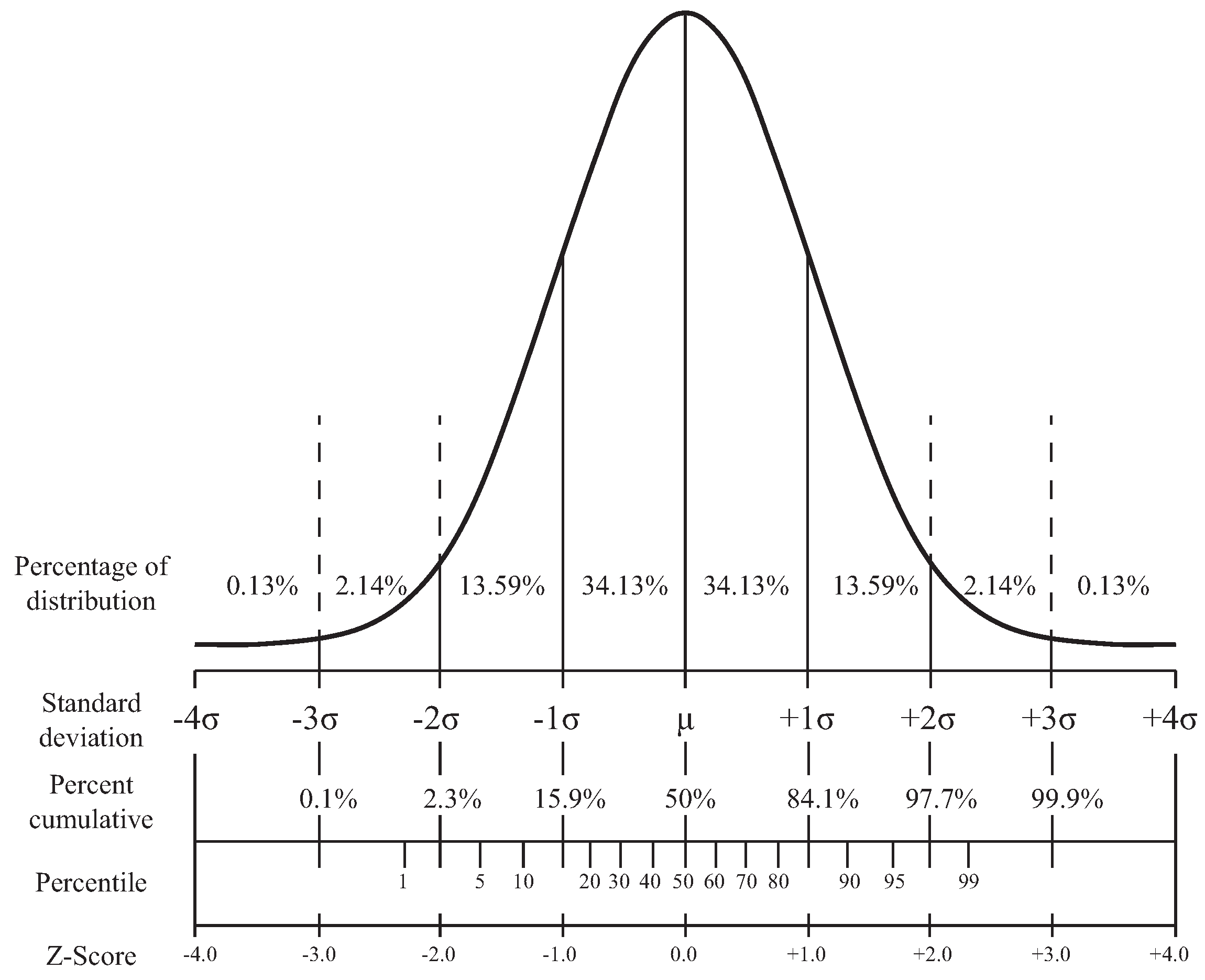
5.1.1. Normal Distribution

Also kwon as the Gaussian distribution, the normal distribution is described by Equation (8), the density of the distribution is given by Equation (9) [64,69,70,71,72,74].

$$F\left(t\right)=\frac{1}{\sigma \sqrt{2\pi }}\underset{-\infty }{\overset{t}{\int }}{e}^{-\frac{{(y-m)}^2}{2{\sigma }^2}}dy=\frac{1}{\sqrt{2\pi }}\underset{-\infty }{\overset{\frac{t-m}{\sigma }}{\int }}{e}^{-\frac{x^2}{2}}dx,-\infty <t,m<\infty ,\sigma >0$$

(8)

$$f\left(t\right)=\frac{1}{\sigma \sqrt{2\pi }}{e}^{-\frac{{(t-m)}^2}{2{\sigma }^2}},-\infty <t,m<\infty ,\sigma >0$$

(9)

5.1.2. Lognormal Distribution

The lognormal distribution is defined by Equation (10), the density of the distribution is given by Equation (11) [69,71,72].

$$\begin{array}{c}F\left(t\right)=\frac{1}{\sigma \sqrt{2\pi }}\underset{0}{\overset{t}{\int }}\frac{1}{y}{e}^{-\frac{{\left(ln\left(\lambda y\right)\right)}^2}{2{\sigma }^2}}dy=\frac{1}{\sqrt{2\pi }}\underset{-\infty }{\overset{\frac{ln\left(\lambda t\right)}{\sigma }}{\int }}{e}^{-\frac{x^2}{2}}dx=\Phi (ln\left(\lambda t\right)/\sigma ),\hfill \\ \\ t\ge 0,\lambda ,\sigma >0\hfill \end{array}$$

(10)

$$f\left(t\right)=\frac{1}{t\sigma \sqrt{2\pi }}{e}^{-\frac{{\left(ln\lambda t\right)}^2}{2{\sigma }^2}},t\ge 0,\lambda ,\sigma >0$$

(11)

5.1.3. Exponential Distribution

The exponential distribution is defined by Equation (12), the density of the distribution is given by Equation (13) [64,69,72,74].

$$F\left(t\right)=1-e^{-\lambda t},t\ge 0,\lambda >0$$

(12)

$$f\left(t\right)=\lambda e^{-\lambda t},t\ge 0,\lambda >0$$

(13)

5.1.4. Weibull Distribution

The weibull distribution is defined by Equation (14), the density of the distribution is given by Equation (15) [64,69,70].

$$F\left(t\right)=1-e^{-{\left(\lambda t\right)}^{\beta }},t\ge 0,\lambda ,\beta >0$$

(14)

$$f\left(t\right)=\lambda \beta {\left(\lambda t\right)}^{\beta -1}{e}^{-{\left(\lambda t\right)}^{\beta }},t\ge 0,\lambda ,\beta >0$$

(15)

5.1.5. Gumbel Distribution

The gumbel distribution is defined by Equation (16), the density of the distribution is given by Equation (17) [74].

$$F\left(t\right)=1-e^{-e^{\frac{t-\mu }{\sigma }}},-\infty <\mu <\infty ,\sigma >0$$

(16)

$$f\left(t\right)=\frac{1}{\sigma }{e}^{z-e^z},wherez=\frac{t-\mu }{\sigma },-\infty <\mu <\infty ,\sigma >0$$

(17)

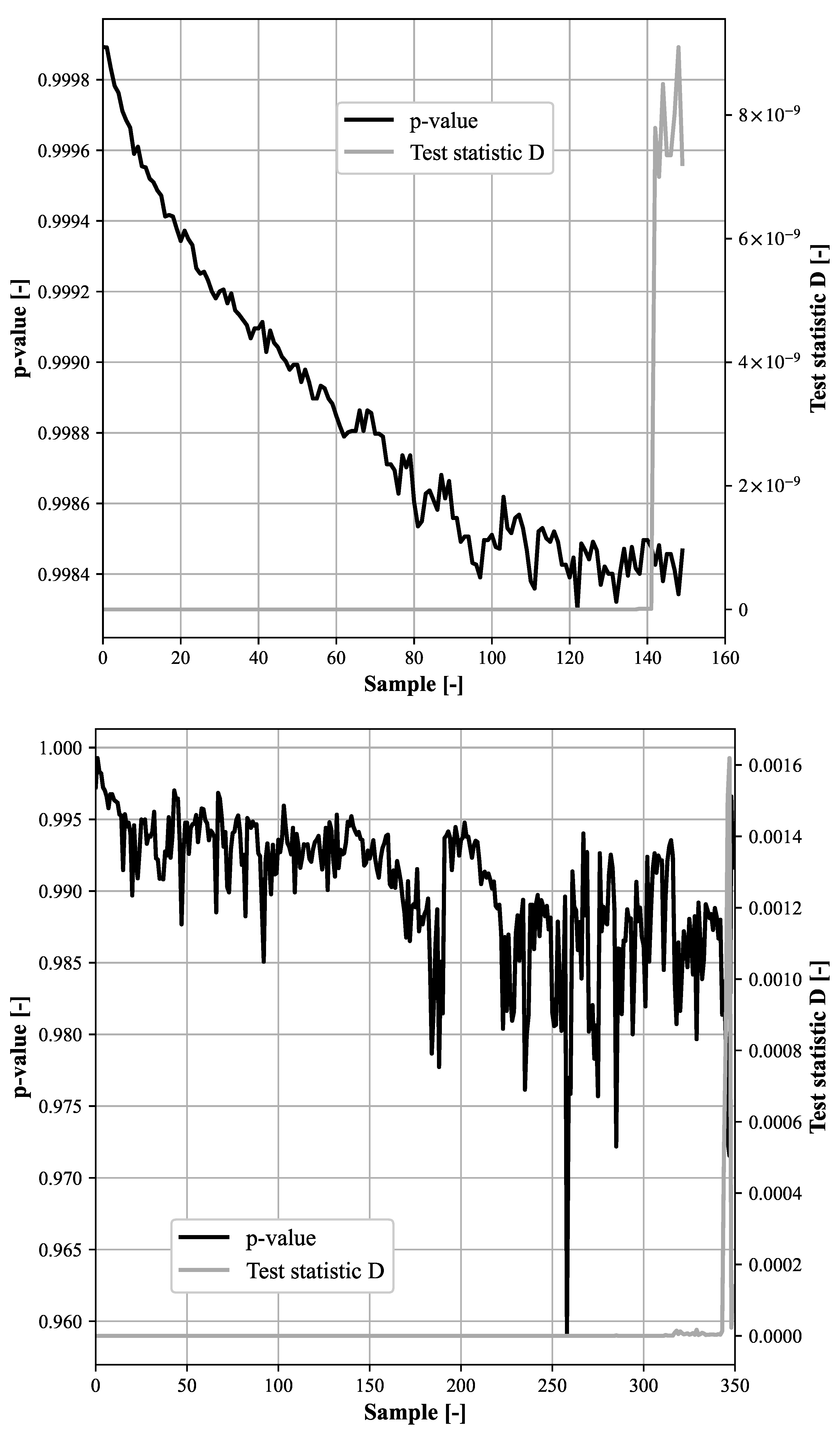
5.2. Goodness of Fit Tests

Figure 12 shows the histogram of an exemplary data set and various distribution models as an overview.

To determine a distribution function for the data set, various goodness-of-fit tests are applicable. In order to compare which distribution model best fits the available measurement data, the values AIC (Akaike information criterion) and BIC (Bayesian information criterion) are first determined for all relevant distribution models [74,75,76]. Both values make it possible to compare the considered distribution models in such a way that a statement can be made whether one distribution model fits the measured data better than the others. In the second step, a Kolmogoroff-Smirnoff test (K-S test) is performed for the distribution models which are considered on the basis of the AIC and BIC values. The K-S test quantifies the goodness of the fit of a given distribution (e.g., a normal distribution) to an observed data set [69,77].

First, the K-S test determines the the largest deviation $D_n$ between an obtained (${\widehat{F}}_n\left(t\right)$) and a given ($F_0\left(t\right)$) function using the following Equation (18) [69,77]:

$$D_n=\underset{-inf<t<inf}{sup}|{\widehat{F}}_n\left(t\right)-F_0\left(t\right)|$$

(18)

$$H_0:F\left(t\right)=F_0\left(t\right)$$

(19)

The null hypothesis (Equation (19)) that both distributions are equal is rejected when the distance $D_n$ exceeds a critical value ($y_{1-a}$). The critical value $y_{1-a}$ depends on the sample size as well as the significance level and can be determined using the table for the Kolmogorov-Smirnov Test in [69].

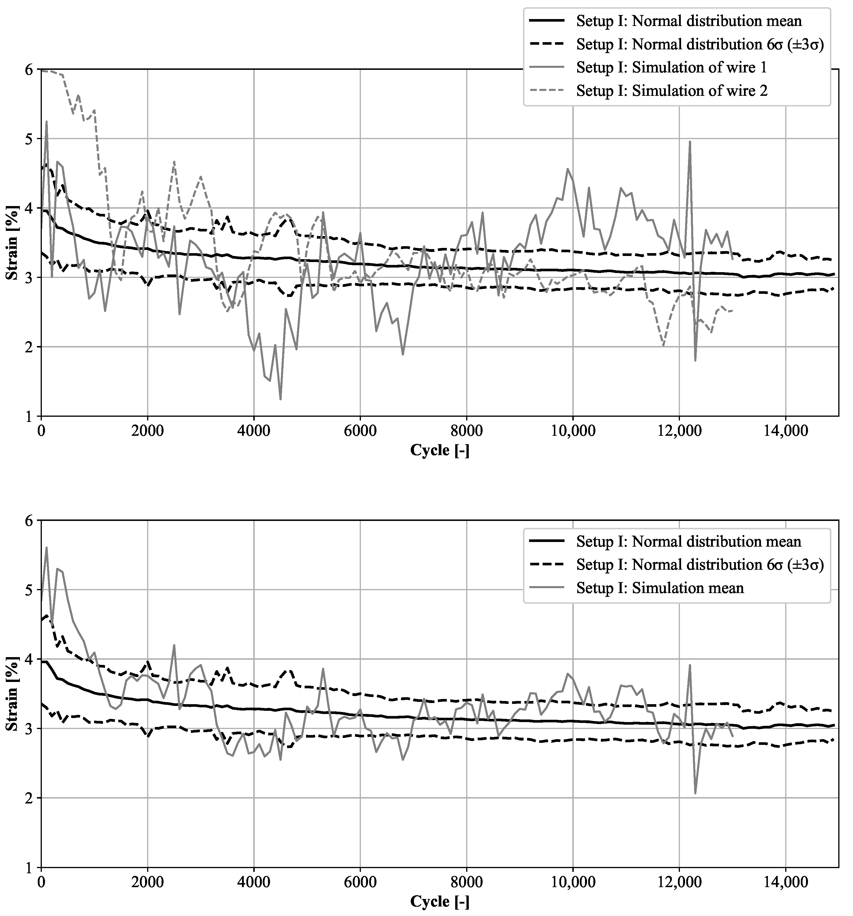
5.3. Approach for the Target Model

For the development of the target model, all tests of test setup I as well as test setup $II$ from Table 1 are used in each case. In order to determine a distribution model for each 100th cycle, the corresponding values of each 100th cycle are combined to a sample. A minimum sample size is required. Since the number of still intact wires decreases along the number of cycles, no distribution model can be determined for the last samples. The target model is created in the following steps:

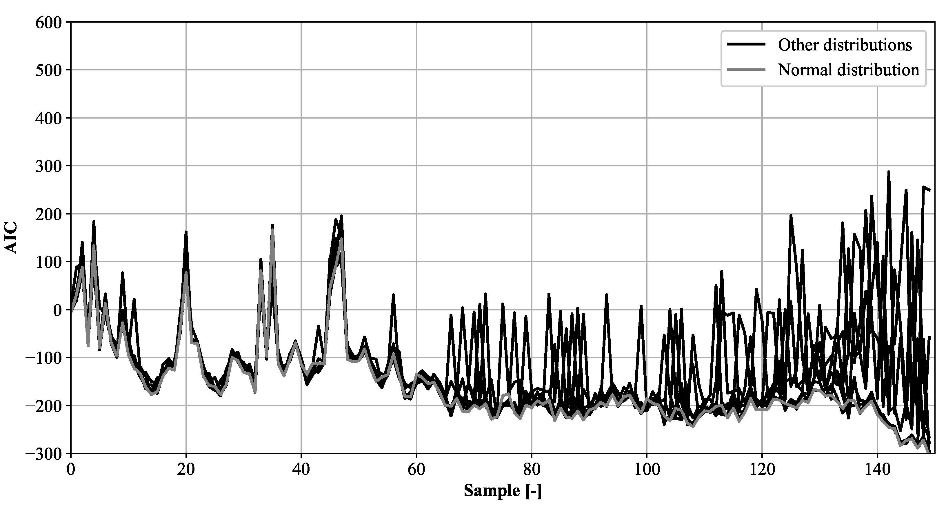
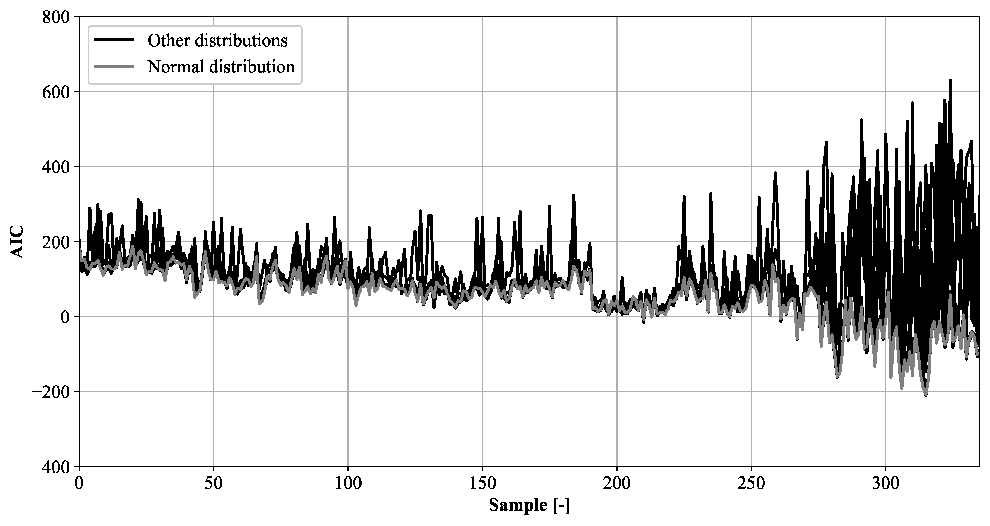
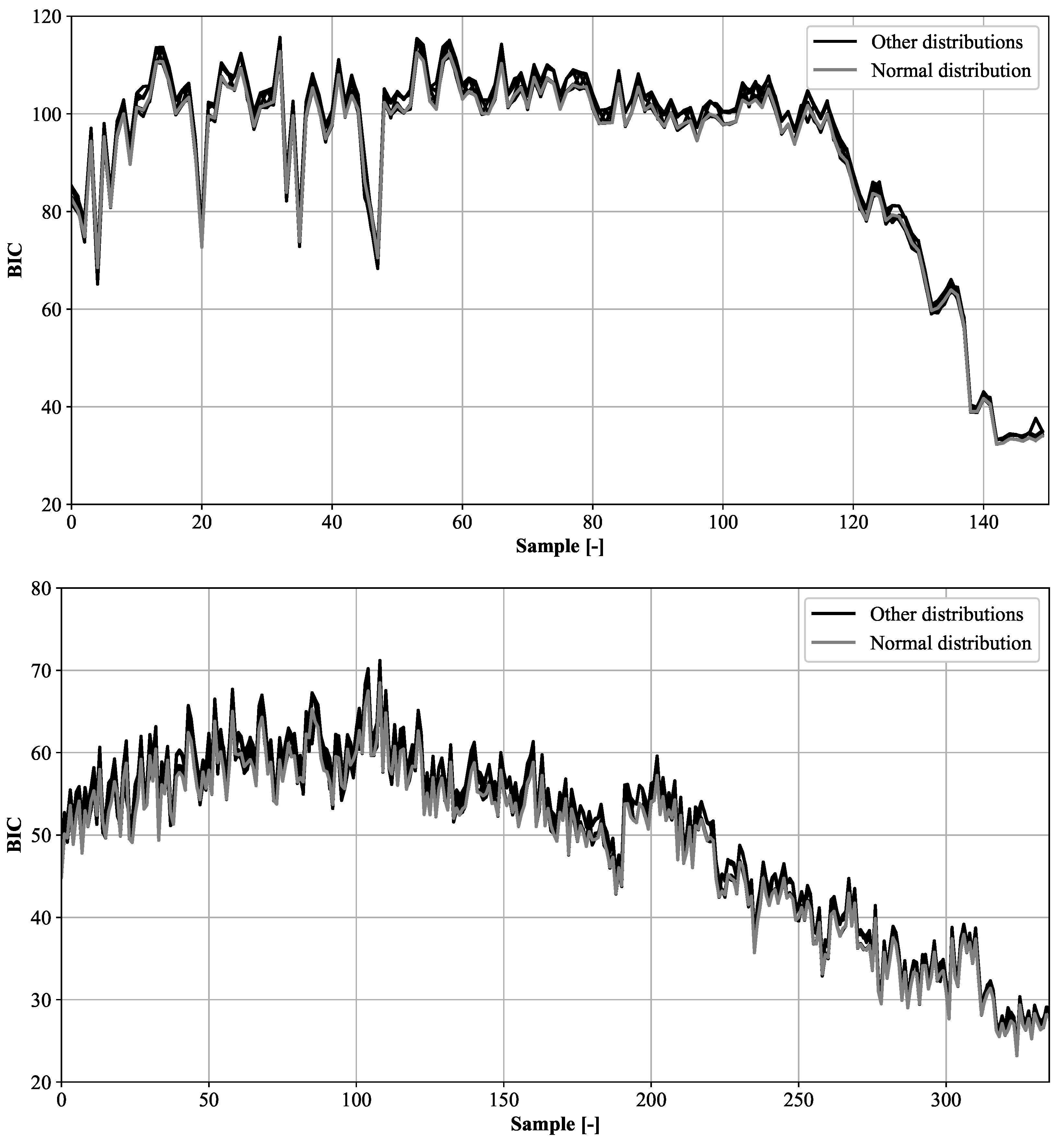
• Calculation of AIC- and BIC-values to determine the appropriate distribution
• Performing a KS-test to approve the fit of the distribution
• Fitting each sample to the distribution
• Determining the $6\sigma$ standard deviation ($\pm 3\sigma$) for each sample (Figure 13)

The overview based on the AIC and BIC values shows that the normal function does not fit the fatigue test data of Setup I and $II$ significantly better or worse than the other distribution models. The corresponding plots of the value curves are shown in the Appendix A—Additional plots (Figure A1 and Figure A2). AIC: In Setup I, the first deviations appear sporadically only after 6000 cycles (60 samples). Only at the end of the tests, from 10,000 cycles, the deviations become larger and more frequent, which is due to the decreasing sample size. Setup $II$, on the other hand, has slight deviations over most of the test time. Only after 25,000 cycles do the deviations increase strongly, again due to the decreasing sample size. BIC: For both setups, there are hardly any deviations over the entire test time.

Since for both setups the normal distribution seems to be as suitable as the other investigated distribution models, a K-S test for normal distribution is performed for both setups in the following step. The corresponding plots are shown in Appendix A—Additional plots (Figure A3). Since for both setups the largest deviation $D_n$ (setup I: ≤1${}^{-9}$, setup $II$: ≤0.00405) is below the critical value $y_{1-a}$ (setup I: 0.237, setup $II$: 0.266) for all samples, the null hypothesis (that the data fits a normal distribution) is not rejected. The associated p-values are $p\ge 0.998$ (setup I) and $p\ge 0.96$ (setup $II$). The target model is therefore developed so that the experimental data are always subject to a normal distribution. For each sample, the normal distribution is fitted based on the available measured values of the tests. In order to narrow down the target range and to enable a qualitative statement, the 6$\sigma$ range is determined in the last step (cf. Figure 13). 99.7% of all measured values are then in the $\mu \pm 3\sigma$ range [69,71,78]. 3$\sigma$ and −3$\sigma$, respectively, thus form the specification limits for the target model.

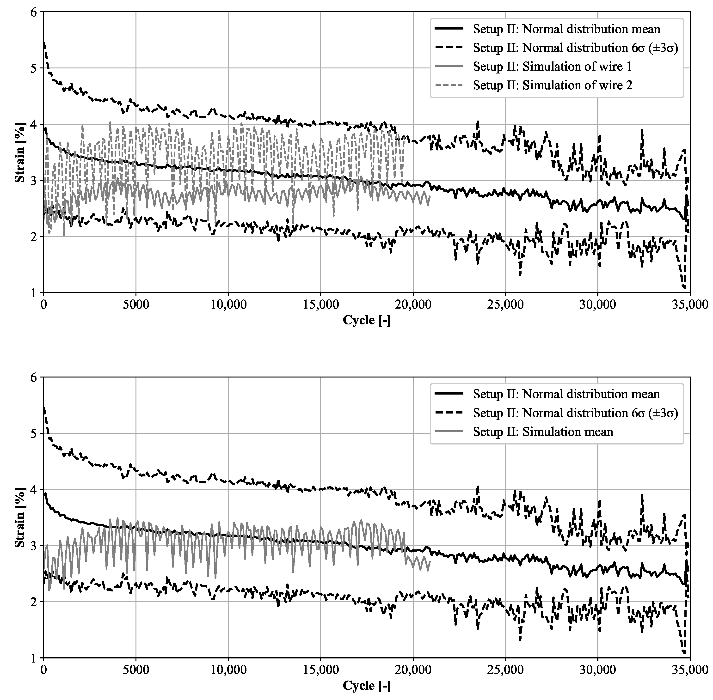
5.4. Final Target Model

The final target models as well as the results of the simulations of both setups are shown in Figure 14 and Figure 15. The target model of setup I is based on 19 from a total of 30 wires that were tested (see Table 1). The other 11 wires were not used for modeling because data analysis determined that implausible value curves were present and anomalies occurred during the tests (e.g., due to insufficient clamping forces). The target model of setup $II$ is based on 15 of 18 tested wires. Figure 14 (Top) shows the comparison of the target model of setup I and two simulated wires. Both simulations repeatedly deviate significantly from the target model throughout the course. Both simulations also differ from each other, so that each simulation deviates significantly different from the other. The mean value of both simulations (Bottom), on the other hand, deviates from the target model less frequently and much more weakly. With the assumption that the simulation is also based on a distribution model, outliers and scattering of the individual simulations must also be taken into account here. However, since only two simulations are available, this is currently not possible. The simulations of setup $II$ are within the target model (Figure 15). Both the individual simulations (Top) and the corresponding average value of both simulations (Bottom) deviate slightly from the target model only within the first 1000 cycles. However, it is noticeable that the second simulated wire scatters significantly more than the first wire. Despite this stronger scattering, the simulation still lies in the target model. As with setup I, further simulations are required if a distribution model is to be considered for the simulations of setup $II$.

6. Verification of the Simulation Model

Within this chapter we take a deeper look into the results. During the operation of the experiments, the development of the model and the analysis of the data, the authors found several interesting indications that are worth investigating beyond this work and the primary leading questions. Three major influences on the applicability of the model and its general accuracy were investigated: the convection, the temperature distribution along the wire and the overall accuracy of the measuring equipment.

6.1. Measuring Equipment

In Figure 11 the deviation between simulation and experiment is exemplarily shown for Setup I performed on the second test rig with the equipment of higher quality (Figure 8). A deeper look into the simulation revealed the following: The activation of 1 s respectively 3 s did not always generate the same amount of measuring points that were expected for the programmed frequency. That means that 1 s of activation time at a frequency of 20 Hz or 50 Hz did not result in 20 or 50 measuring points but 2–3 measuring points more or less resulting in a slightly longer or shorter activation time. This effect is part of the reason why the resulting stroke is not a thin line but a bold line (see Figure 1, Figure 4 and Figure 10). However, the deviation in the activation time seems to have a greater impact on the simulation than for the experiment. This might be a hint for a missing effect in the simulation model. If the predicted stroke based on the measured values scatter more than the values for the stroke from the experiment there might be some kind of damping factor that was not taken into account.

6.2. Convection

One factor with a great influence on the activation behavior is the convection. As a general approach the energy loss due to convection is between 10% and 20% [79]. For obvious reasons a range of this size makes it hard to precisely predict the loss due to thermal convection. Furthermore the heating process is time-dependent: The wire heats up, resulting in a thin layer of heated air around the wire. This layer affects the heat transfer coefficient since it is temperature dependent and thefore the convection. On top of that, it is well known that a change of the ambient temperature of a few degrees strongly influences the activation behaviour [12]. Since the wires are very thin the mounting of the wire, whether vertical or horizontal, also affects the heat transfer. The warm air around the wire rises, therefore the heated air film disappears faster for a horizontal mounting compared to a vertical mounting. All these factors make it hard to properly estimate the energy loss due to convection without a comprehensive CFD-Analysis. Still, such a simulation can only generate proper results for a certain set of parameters. If the boundary conditions change, the simulation does not fit anymore. All these reasons makes it nearly impossible to perfectly predict the resulting strain.

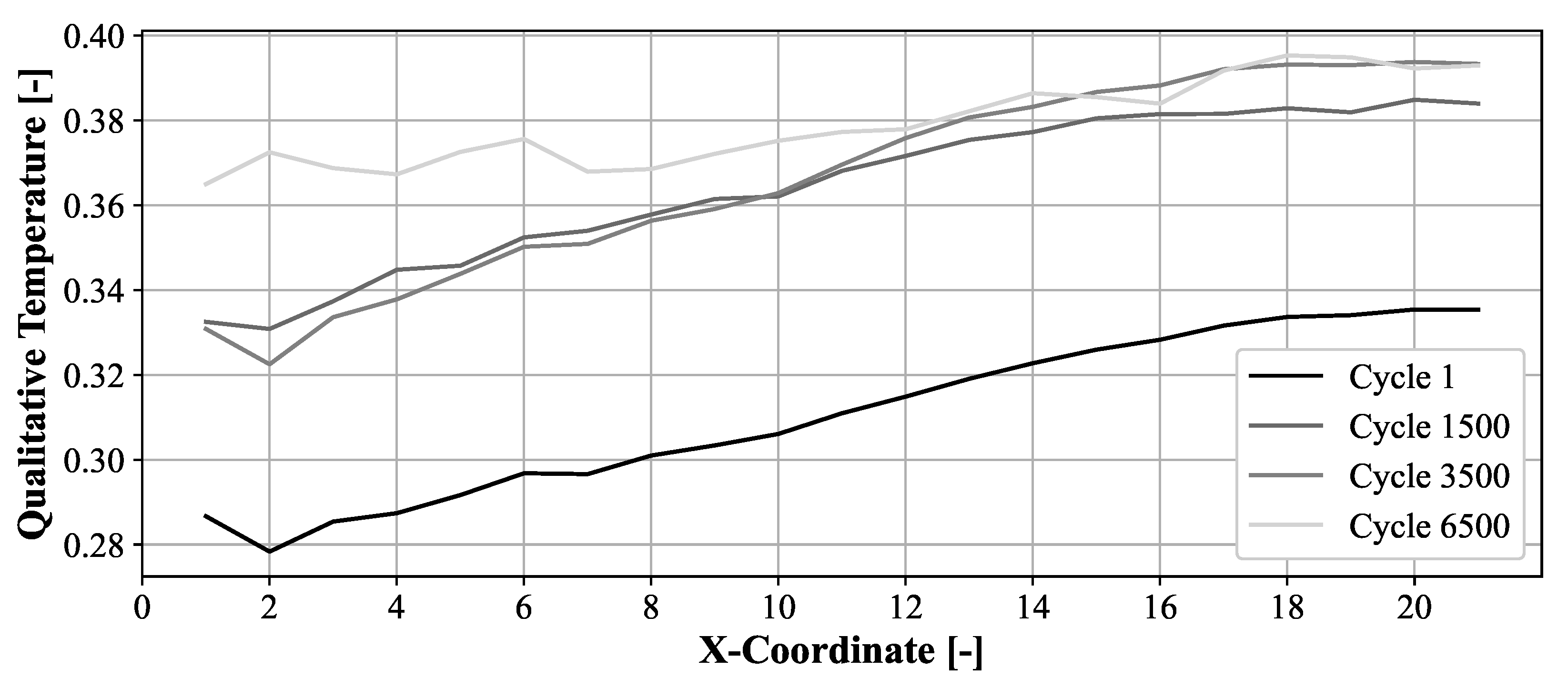
6.3. Temperature Distribution

The results from [80] found that with increasing cycle count, hotspots in the temperature distribution along the wire emerge. In this work, the temperature distribution of the wire specimen was monitored by a thermal imaging camera and the qualitative temperature was analyzed. The leading question was: Is it possible to monitor the formation of cracks that decrease the wires cross section and therefore locally increase the electric resistance via thermography? A locally increased electric resistance also increases the local temperature. The study found hotspots at positions where the wire finally broke. The qualitative temperature was shown and not the absolute temperature since thermography of the SMA wires is challenging: The objects are of small diameter, round and the emission coefficient is not constant during activation. Along with the rather low temperature range between 20 °C and 150 °C, measuring the correct absolute temperature contactless by thermography is very costly. Furthermore, the absolute temperature does not contribute to the question of a varying temperature distribution.

The experiment was repeated once for a specimen of setup $II$ to check if this effect is repeatable. The results are shown in Figure 16. The results shown along with [80] indicate that contrary to the assumption of the simulation model, the wire does not heat constantly but with increased cycle-count some parts are hotter and some are cooler. The experiments indicate that there might be an influence on the model’s accuracy since the model assumes a constant temperature distribution.

7. Conclusions

In this work, a simulation model was developed to predict the strain of an SMA wire based on the energy input. Previous approaches neglected degradation effects from structural and functional fatigue and were therefore only applicable for new wires that were not previously activated. Activating the wires changes their PTT and leads to a different energy consumption to generate strain. In this work, the electric resistance was monitored since it is the measurand that is strongly linked to the degradation behavior of SMA components.

Alongside the simulation model, two statistically valid target models for two different load scenarios were derived. The target models show the normal distribution of the strain resulting from the load scenario. These models were developed to investigate the applicability of the simulation model. In addition, this enables forecasts of the (remaining) lifetime during operation.

The strain prediction for setup $II$ was generally more accurate than the results for test setup I. As the main influences are the measuring accuracy, the convection, and the temperature distribution along the wire. All factors contribute to a deviation between simulation results and the target model. The results of setup $II$ are however still promising. The goal of the simulation model is to enable strain control during the operation of an SMA component. Further investigation to increase the accuracy of the simulation model is needed.

References

1. Otsuka, K. (Ed.) Shape Memory Materials, 1st ed.; Cambridge University Press: Cambridge, UK, 1998. [Google Scholar]
2. Lagoudas, D.C. Shape Memory Alloys: Modeling and Engineering Applications; Springer: Boston, MA, USA, 2008. [Google Scholar] [CrossRef]
3. Lexcellent, C. Shape Memory Alloys Handbook; Materials Science Series; ISTE: London, UK, 2013. [Google Scholar]
4. Rao, A.; Srinivasa, A.R.; Reddy, J.N. Design of Shape Memory Alloy (SMA) Actuators; Springer Briefs in Applied Sciences and Technology; Springer International Publishing: Cham, Switzerland, 2015. [Google Scholar] [CrossRef]
5. Gümpel, P.; Gläser, S.; Jost, N.; Mertmann, M.; Seitz, N.; Strittmatter, J. Formgedächtnislegierungen: Einsatzmöglichkeiten in Maschinenbau, Medizintechnik und Aktuatorik, 2nd ed.; Volume Band 655; Kontakt & Studium Expert Verlag: Renningen, Germany, 2018. [Google Scholar]
6. Janocha, H. (Ed.) Adaptronics and Smart Structures: Basics, Materials, Design, and Applications; with 17 Tables, 2nd ed.; Springer: Berlin/Heidelberg, Germany, 2007. [Google Scholar]
7. Mohd Jani, J.; Leary, M.; Subic, A.; Gibson, M.A. A review of shape memory alloy research, applications and opportunities. Mater. Des. (1980–2015) 2014, 56, 1078–1113. [Google Scholar] [CrossRef]
8. Stöckel, D. Legierungen mit Formgedächtnis: Industrielle Nutzung d. Shape-Memory-Effektes; Grundlagen, Werkstoffe, Anwendungen; Volume 259 Werkstoffe; Kontakt & Studium, Expert-Verl.: Ehningen bei Böblingen, Germany, 1988. [Google Scholar]
9. Lygin, K. Eine Methodik zur Entwicklung von Umgebungsaktivierten FG-Aktoren Mit Geringer Thermischer Hysterese am Beispiel der Heizungs- und Klimatechnik. Ph.D. Thesis, Ruhr-Universität Bochum, Bochum, Germany, 2014. [Google Scholar]
10. Schiedeck, F. Entwicklung Eines Modells für Formgedächtnisaktoren im Geregelten Dynamischen Betrieb. Ph.D. Thesis, PZH Produktionstechnisches Zentrum Hannover, Garbsen, Germany, 2009. [Google Scholar]
11. Stoeckel, D. Shape memory actuators for automotive applications. Mater. Des. (1980–2015) 1990, 11, 302–307. [Google Scholar] [CrossRef]
12. Otibar, D.; Weirich, A.; Kortenjann, M.; Kuhlenkötter, B. A Preliminary Investigation of Temperature Dependency of a Shape Memory Actuator with Time-Based Control in Aircraft Interiors. IOP Conf. Ser. Mater. Sci. Eng. 2017, 216, 012009. [Google Scholar] [CrossRef] [Green Version]
13. Kuhlenkötter, W. Applicability of Shape Memory Alloys in Aircraft Interiors. Actuators 2019, 8, 61. [Google Scholar] [CrossRef] [Green Version]
14. Barbarino, S.; Saavedra Flores, E.I.; Ajaj, R.M.; Dayyani, I.; Friswell, M.I. A review on shape memory alloys with applications to morphing aircraft. Smart Mater. Struct. 2014, 23, 063001. [Google Scholar] [CrossRef]
15. Costanza, G.; Tata, M.E. Shape Memory Alloys for Aerospace, Recent Developments, and New Applications: A Short Review. Materials 2020, 13, 1856. [Google Scholar] [CrossRef] [Green Version]
16. Duerig, T.; Pelton, A.; Stöckel, D. An overview of nitinol medical applications. Mater. Sci. Eng. A 1999, 273–275, 149–160. [Google Scholar] [CrossRef]
17. Jiang, S.; Chen, B.; Qi, F.; Cao, Y.; Ju, F.; Bai, D.; Wang, Y. A variable-stiffness continuum manipulators by an SMA-based sheath in minimally invasive surgery. Int. J. Med. Robot. Comput. Assist. Surg. MRCAS 2020, 16, e2081. [Google Scholar] [CrossRef]
18. Spaggiari, A.; Castagnetti, D.; Golinelli, N.; Dragoni, E.; Scirè Mammano, G. Smart materials: Properties, design and mechatronic applications. J. Mater. Des. Appl. 2019, 233, 734–762. [Google Scholar] [CrossRef]
19. Gopal, V.; Alphin, M.S.; Bharanidaran, R. Design of Compliant Mechanism Microgripper Utilizing the Hoekens Straight Line Mechanism. J. Test. Eval. 2021, 49, 20190091. [Google Scholar] [CrossRef]
20. Jeong, J.; Yasir, I.B.; Han, J.; Park, C.H.; Bok, S.K.; Kyung, K.U. Design of Shape Memory Alloy-Based Soft Wearable Robot for Assisting Wrist Motion. Appl. Sci. 2019, 9, 4025. [Google Scholar] [CrossRef] [Green Version]
21. Liu, M.; Hao, L.; Zhang, W.; Zhao, Z. A novel design of shape-memory alloy-based soft robotic gripper with variable stiffness. Int. J. Adv. Robot. Syst. 2020, 17, 172988142090781. [Google Scholar] [CrossRef]
22. Manfredi, L.; Cuschieri, A. Design of a 2 DOFs Mini Hollow Joint Actuated with SMA Wires. Materials 2018, 11, 2014. [Google Scholar] [CrossRef] [Green Version]
23. Motzki, P.; Seelecke, S.; Rizzello, G. A Shape Memory Alloy Smart Handling System for Advanced Manufacturing Applications. In Proceedings of the 2020 7th International Conference on Control, Decision and Information Technologies (CoDIT), Prague, Czech Republic, 29 June–2 July 2020; pp. 229–234. [Google Scholar] [CrossRef]
24. Elahinia, M.; Shayesteh Moghaddam, N.; Taheri Andani, M.; Amerinatanzi, A.; Bimber, B.A.; Hamilton, R.F. Fabrication of NiTi through additive manufacturing: A review. Prog. Mater. Sci. 2016, 83, 630–663. [Google Scholar] [CrossRef] [Green Version]
25. Haberland, C.; Elahinia, M.; Walker, J.M.; Meier, H.; Frenzel, J. On the development of high quality NiTi shape memory and pseudoelastic parts by additive manufacturing. Smart Mater. Struct. 2014, 23, 104002. [Google Scholar] [CrossRef]
26. Nigito, E.; Diemer, F.; Husson, S.; Ou, S.F.; Tsai, M.H.; Rézaï-Aria, F. Microstructure of NiTi superelastic alloy manufactured by selective laser melting. Mater. Lett. 2022, 324, 132665. [Google Scholar] [CrossRef]
27. Saedi, S.; Shayesteh Moghaddam, N.; Amerinatanzi, A.; Elahinia, M.; Karaca, H.E. On the effects of selective laser melting process parameters on microstructure and thermomechanical response of Ni-rich NiTi. Acta Mater. 2018, 144, 552–560. [Google Scholar] [CrossRef]
28. Zeng, Z.; Cong, B.; Oliveira, J.P.; Ke, W.; Schell, N.; Peng, B.; Qi, Z.W.; Ge, F.; Zhang, W.; Ao, S.S. Wire and arc additive manufacturing of a Ni-rich NiTi shape memory alloy: Microstructure and mechanical properties. Addit. Manuf. 2020, 32, 101051. [Google Scholar] [CrossRef]
29. Seelecke, S. Sensing Properties of SMA Actuators and Sensorless Control. In Shape Memory Alloy Valves; Czechowicz, A., Langbein, S., Eds.; Springer International Publishing: Cham, Switzerland, 2015; pp. 73–87. [Google Scholar] [CrossRef]
30. Theren, B.; Heß, P.; Bracke, S.; Kuhlenkötter, B. Influence of the phase transformation behavior of NiTi shape memory alloy wires on the predictability of strain during operation. In Proceedings of the ASME 2022 Conference on Smart Materials, Adaptive Structures and Intelligent Systems, Detroit, MI, USA, 12–14 September 2022. [Google Scholar]
31. Heß, P.; Bracke, S. An Approach to Predict the Lifetime of Shape Memory Actuators based on Accelerated Testing Measurements. In Proceedings of the 30th European Safety and Reliability Conference and 15th Probabilistic Safety Assessment and Management Conference, Venice, Italy, 1–5 November 2020; Baraldi, P., Di Maio, F., Zio, E., Eds.; Research Publishing Services: Singapore, 2020; pp. 1528–1535. [Google Scholar] [CrossRef]
32. Heß, P.; Bracke, S. Zuverlässigkeitstechnik bei Formgedächtnisaktoren: Entwicklung von Prüfstandstechnik und Erprobungsprogramm. In Potenziale Künstlicher Intelligenz für die Qualitätswissenschaft: Bericht zur GQW-Jahrestagung 2018 in Nürnberg; Gesellschaft für Qualitätswissenschaft e.V., Ed.; Springer: Berlin/Heidelberg, Germany, 2018. [Google Scholar]
33. Heß, P.; Bracke, S. Reliability and degradation analysis of smart material actuators. In Proceedings of the 29th European Safety and Reliability Conference (ESREL 2019), Hannover, DE, USA, 22–26 September 2019; Beer, M., Zio, E., Eds.; Research Publishing Services: Singapore, 2019. [Google Scholar]
34. Heß, P.; Bracke, S. Smart material actuators as a contributor for IoT-based smart applications and systems: Analyzing prototype and process measurement data of shape memory actuators for reliability and risk prognosis. J. Adv. Mech. Des. Syst. Manuf. 2020, 14, JAMDSM0026. [Google Scholar] [CrossRef] [Green Version]
35. Heß, P.; Bracke, S. Estimation of the Remaining Lifetime of Shape Memory Alloy Actuators during Prototype Testing: Analysis of the Impact Of Different Currents. In Proceedings of the 31st European Safety and Reliability Conference (ESREL 2021), Angers, France, 19–23 September 2021; Castanier, B., Cepin, M., Bigaud, D., Berenguer, C., Eds.; Research Publishing Services: Singapore, 2021; pp. 3170–3177. [Google Scholar] [CrossRef]
36. Kang, G.; Song, D. Review on structural fatigue of NiTi shape memory alloys: Pure mechanical and thermo-mechanical ones. Theor. Appl. Mech. Lett. 2015, 5, 245–254. [Google Scholar] [CrossRef] [Green Version]
37. You, Y.; Zhang, Y.; Moumni, Z.; Anlas, G.; Zhang, W. Effect of the thermomechanical coupling on fatigue crack propagation in NiTi shape memory alloys. Mater. Sci. Eng. A 2017, 685, 50–56. [Google Scholar] [CrossRef]
38. Rahim, M.; Frenzel, J.; Frotscher, M.; Pfetzing-Micklich, J.; Steegmüller, R.; Wohlschlögel, M.; Mughrabi, H.; Eggeler, G. Impurity levels and fatigue lives of pseudoelastic NiTi shape memory alloys. Acta Mater. 2013, 61, 3667–3686. [Google Scholar] [CrossRef]
39. Robertson, S.W.; Pelton, A.R.; Ritchie, R.O. Mechanical fatigue and fracture of Nitinol. Int. Mater. Rev. 2012, 57, 1–37. [Google Scholar] [CrossRef]
40. Robertson, S.W.; Launey, M.; Shelley, O.; Ong, I.; Vien, L.; Senthilnathan, K.; Saffari, P.; Schlegel, S.; Pelton, A.R. A statistical approach to understand the role of inclusions on the fatigue resistance of superelastic Nitinol wire and tubing. J. Mech. Behav. Biomed. Mater. 2015, 51, 119–131. [Google Scholar] [CrossRef]
41. Zhang, J.; Somsen, C.; Simon, T.; Ding, X.; Hou, S.; Ren, S.; Ren, X.; Eggeler, G.; Otsuka, K.; Sun, J. Leaf-like dislocation substructures and the decrease of martensitic start temperatures: A new explanation for functional fatigue during thermally induced martensitic transformations in coarse-grained Ni-rich Ti–Ni shape memory alloys. Acta Mater. 2012, 60, 1999–2006. [Google Scholar] [CrossRef]
42. Grossmann, C.; Frenzel, J.; Sampath, V.; Depka, T.; Eggeler, G. Elementary Transformation and Deformation Processes and the Cyclic Stability of NiTi and NiTiCu Shape Memory Spring Actuators. Metall. Mater. Trans. A 2009, 40, 2530–2544. [Google Scholar] [CrossRef]
43. Auricchio, F.; Taylor, R.L.; Lubliner, J. Shape-memory alloys: Macromodelling and numerical simulations of the superelastic behavior. Comput. Methods Appl. Mech. Eng. 1997, 146, 281–312. [Google Scholar] [CrossRef]
44. Bhattacharya, K.; Conti, S.; Zanzotto, G.; Zimmer, J. Crystal symmetry and the reversibility of martensitic transformations. Nature 2004, 428, 55–59. [Google Scholar] [CrossRef] [Green Version]
45. Seelecke, S.; Muller, I. Shape memory alloy actuators in smart structures: Modeling and simulation. Appl. Mech. Rev. 2004, 57, 23–46. [Google Scholar] [CrossRef]
46. Shaw, J.A. Simulations of localized thermo-mechanical behavior in a NiTi shape memory alloy. Int. J. Plast. 2000, 16, 541–562. [Google Scholar] [CrossRef]
47. Xiao, Y.; Jiang, D. Thermomechanical modeling on cyclic deformation and localization of superelastic NiTi shape memory alloy. Int. J. Solids Struct. 2022, 250, 111723. [Google Scholar] [CrossRef]
48. Shayanfard, P.; Heller, L.; Šandera, P.; Šittner, P. Numerical analysis of NiTi actuators with stress risers: The role of bias load and actuation temperature. Eng. Fract. Mech. 2021, 244, 107551. [Google Scholar] [CrossRef]
49. Elahinia, M. Effect of System Dynamics on Shape Memory Alloy Behavior and Control. Ph.D. Thesis, Virginia Tech, Blacksburg, VA, USA, 2004. [Google Scholar]
50. Elahinia, M.H. Shape Memory Alloy Actuators: Design, Fabrication, and Experimental Evaluation; John Wiley and Sons Inc.: Chichester, UK, 2015. [Google Scholar]
51. Pagel, K.; Drossel, W.G.; Zorn, W. Multi-functional Shape-Memory-Actuator with guidance function. Prod. Eng. 2013, 7, 491–496. [Google Scholar] [CrossRef]
52. Pagel, K. Entwicklung von Formgedächtnisaktoren mit Inhärenter Führungsfunktion. Ph.D. Thesis, Technische Universität Chemnitz, Auerbach Verlag Wissenschaftliche Scripten, Vogtland, Germany, 2018. [Google Scholar]
53. Meier, H.; Oelschlaeger, L. Numerical thermomechanical modelling of shape memory alloy wires. Mater. Sci. Eng. A 2004, 378, 484–489. [Google Scholar] [CrossRef]
54. Oelschläger, L. Numerische Modellierung des Aktivierungsverhaltens von Formgedächtnisaktoren am Beispiel Eines Schrittantriebes. Ph.D. Thesis, Schriftenreihe des Lehrstuhls für Produktionssysteme, Institut für Automatisierungstechnik, Lehrstuhl für Produktionssysteme, Shaker, Aachen, Germany, 2004. [Google Scholar]
55. Shayanfard, P.; Kadkhodaei, M.; Jalalpour, A. Numerical and Experimental Investigation on Electro-Thermo-Mechanical Behavior of NiTi Shape Memory Alloy Wires. Iran. J. Sci. Technol. Trans. Mech. Eng. 2019, 43, 621–629. [Google Scholar] [CrossRef]
56. Kalra, S.; Bhattacharya, B.; Munjal, B.S. Design of shape memory alloy actuated intelligent parabolic antenna for space applications. Smart Mater. Struct. 2017, 26, 095015. [Google Scholar] [CrossRef]
57. Bhargaw, H.N.; Ahmed, M.; Sinha, P. Thermo-electric behaviour of NiTi shape memory alloy. Trans. Nonferrous Met. Soc. China 2013, 23, 2329–2335. [Google Scholar] [CrossRef]
58. Sreekumar, M.; Singaperumal, M.; Nagarajan, T.; Zoppi, M.; Molfino, R. Recent advances in nonlinear control technologies for shape memory alloy actuators. J. Zhejiang Univ.-Sci. A 2007, 8, 818–829. [Google Scholar] [CrossRef]
59. Zaidi, S.; Lamarque, F.; Favergeon, J.; Carton, O.; Prelle, C. Wavelength-Selective Shape Memory Alloy for Wireless Microactuation of a Bistable Curved Beam. IEEE Trans. Ind. Electron. 2011, 58, 5288–5295. [Google Scholar] [CrossRef]
60. Liang, C.; Rogers, C.A. One-Dimensional Thermomechanical Constitutive Relations for Shape Memory Materials. J. Intell. Mater. Syst. Struct. 1990, 1, 207–234. [Google Scholar] [CrossRef]
61. Antonucci, V.; Faiella, G.; Giordano, M.; Mennella, F.; Nicolais, L. Electrical resistivity study and characterization during NiTi phase transformations. Thermochim. Acta 2007, 462, 64–69. [Google Scholar] [CrossRef]
62. Theren, B.; Otibar, D.; Weirich, A.; Brandenburg, J.; Kuhlenkötter, B. (Eds.) Methodology for Minimizing Operational Influences of the Test Rig During Long-Term Investigations of SMA Wires. In Proceedings of the ASME 2019 Conference on Smart Materials, Adaptive Structures and Intelligent Systems, Louisville, KY, USA, 9–11 September 2019. [Google Scholar] [CrossRef]
63. Verein Deutscher Ingenieure. VDI 2248-Produktentwicklung mit Formgedächtnislegierungen (FGL); VDI-Guideline; Verein Deutscher Ingenieure: Düsseldorf, Germany, 2017. [Google Scholar]
64. Nelson, W. Accelerated Testing: Statistical Models, Test Plans and Data Analysis; Wiley Series in Probability and Mathematical Statistics; Applied Probability and Statistics; Wiley-Interscience: Hoboken, NJ, USA, 2004. [Google Scholar]
65. Escobar, L.A.; Meeker, W.Q. A Review of Accelerated Test Models. Stat. Sci. 2006, 21, 552–577. [Google Scholar] [CrossRef] [Green Version]
66. Meeker, W.Q.; Escobar, L.A. Statistical Methods for Reliability Data; Wiley Series in Probability and Statistics; Applied Probability and Statistics Section; Wiley: New York, NY, USA, 1998. [Google Scholar]
67. Pascual, F.; Meeker, W.; Escobar, L. Accelerated Life Test Models and Data Analysis. In Springer Handbook of Engineering Statistics; Pham, H., Ed.; Springer: London, UK, 2006; pp. 397–426. [Google Scholar] [CrossRef] [Green Version]
68. Pearson, R.K. Data cleaning for dynamic modeling and control. In Proceedings of the 1999 European Control Conference (ECC), Karlsruhe, Germany, 31 August–3 September 1999; pp. 2584–2589. [Google Scholar] [CrossRef]
69. Birolini, A. Reliability Engineering: Theory and Practice, 3rd ed.; Springer: Berlin/Heidelberg, Germany, 1999. [Google Scholar]
70. Rinne, H. The Weibull Distribution: A Handbook; CRC Press: Boca Raton, FL, USA, 2009. [Google Scholar]
71. Sachs, L. Angewandte Statistik: Anwendung Statistischer Methoden; Elfte, überarbeitete und Aktualisierte Auflage; Springer eBook Collection Life Science and Basic Disciplines; Springer: Berlin/Heidelberg, Germany, 2004. [Google Scholar] [CrossRef]
72. Modarres, M.; Kaminskiy, M.; Krivtsov, V. Reliability Engineering and Risk Analysis: A Practical Guide; Quality and Reliability; Dekker: New York, NY, USA, 1999; Volume 55. [Google Scholar]
73. Hartung, J. Statistik: Lehr- und Handbuch der Angewandten Statistik; Oldenbourg Wissenschaftsverlag: Munchen, Germany, 2012. [Google Scholar]
74. Matthew Reid. MatthewReid854/Reliability: v0.5.1, Documentation of the Python Package Reliability. 2020. Available online: https://reliability.readthedocs.io/en/latest/index.html (accessed on 2 July 2022).
75. Ghosh, J.K.; Delampady, M.; Samanta, T. An Introduction to Bayesian Analysis: Theory and Methods; Springer Texts in Statistics; Springer: New York, NY, USA, 2006. [Google Scholar]
76. Akaike, H. A new look at the statistical model identification. IEEE Trans. Autom. Control 1974, 19, 716–723. [Google Scholar] [CrossRef]
77. Sachs, L. Applied Statistics: A Handbook of Techniques, 2nd ed.; Springer Series in Statistics; Springer: New York, NY, USA, 1984. [Google Scholar]
78. Hedderich, J.; Sachs, L. Angewandte Statistik: Methodensammlung mit R, 16; überarbeitete und Erweiterte Auflage; Springer: Berlin/Heidelberg, Germany, 2018. [Google Scholar]
79. Verein Deutscher Ingenieure. VDI-Wärmeatlas; Springer Vieweg: Berlin/Heidelberg, Germany, 2013. [Google Scholar] [CrossRef]
80. Theren, B.; Kuhlenkötter, B.; Schuleit, M.; Esen, C. A Method of Crack Monitoring for Electrically Activated SMA Wires Using Thermography. In Proceedings of the ASME 2020 Conference on Smart Materials, Adaptive Structures and Intelligent Systems, American Society of Mechanical Engineers, Virtual, 15 September 2020. [Google Scholar] [CrossRef]
Figure 1. Stroke [mm] (Left) and electrical resistance [ Ω ] (Right) over cycles [-] for various load scenarios. Source: [30].
Crystals 12 01121 g001
Figure 2. Decreasing hysteresis for a binary NiTi wire, 0.28 mm diameter at 350 MPa. Source: Cf. [30].
Crystals 12 01121 g002
Figure 3. Maximum of current, voltage, strain, energy and resistance per cycle for a 3% strain. Every 100th cycle was a full activation (5% strain) to further track the degradation of the parameters.
Crystals 12 01121 g003
Figure 4. Degradation of the strain (Right) and the start/end position (Left) for the full activation.
Crystals 12 01121 g004
Figure 5. Test rig for fatigue tests of 3 SMA wires with weight as the resetting element (a) Complete test rig; (b) Detailed view of 1 test channel. Source: [30,31,33,35].
Crystals 12 01121 g005
Figure 6. Measurement series of the endurance test rig showing the measured variables displacement [mm], voltage for activation [V] and force [N] over time [s]. Source: [30].
Crystals 12 01121 g006
Figure 7. Full endurance test ot the test rig of test setup I showing the current [A] and voltage for activation [V], peak values of displacement [mm], ambient temperature [°C], energy [J] and resistance of the wire [ Ω ] over test cycles [n].
Crystals 12 01121 g007
Figure 8. Second test rig for fatigue tests. Source: [62].
Crystals 12 01121 g008
Figure 9. Test rig for fatigue tests of a single SMA wire inside of a climate chamber. Source: [30].
Crystals 12 01121 g009
Figure 10. Input parameters for the plausibility analysis of the model.
Crystals 12 01121 g010
Figure 11. Example of a simulated strain compared to the experiment.
Crystals 12 01121 g011
Figure 12. Example of a histogramm plot of the probability density function and the cumulative distribution function of fitted distributions.
Crystals 12 01121 g012
Figure 13. Area fractions (quantiles) for a normal distribution. Source: cf. [78].
Crystals 12 01121 g013
Figure 14. Target model for setup I based on the fatigue tests: Comparison of target model and 2 simulated wires (Top); Comparison of target model and the mean of the simulation (Bottom).
Crystals 12 01121 g014
Figure 15. Target model for setup I I based on the fatigue tests: Comparison of target model and 2 simulated wires (Top); Comparison of target model and the mean of the simulation (Bottom).
Crystals 12 01121 g015
Figure 16. Change of the temperature distribution along the wire over different numbers of cycles.
Crystals 12 01121 g016