An Isogeometric Bézier Finite Element Method for Vibration Optimization of Functionally Graded Plate with Local Refinement

Abstract

An effective free vibration optimization procedure in combination with the isogeometric approach (IGA), particle swarm optimization (PSO) and an integrated global and local parameterization is presented. The natural frequency of functionally graded (FG) plates is calculated by the IGA based on the Bézier extraction of non-uniform rational B-splines (NURBS) with the cubic NURBS basis function. The material composition is assumed to vary only in the thickness direction, and the volumetric fraction is described by the NURBS basis function in light of the superior properties of NURBS curves. The volume fractions of the control points are then optimized by the PSO. In most of the previous work, the control points for the volume fraction are usually equally spaced, which is incapable of identifying the optimal location of the graded zones in most cases. To overcome this bottleneck, a novel local refinement strategy is proposed. The reliability and effectiveness of the proposed approach are demonstrated through several numerical examples. It is interesting to observe that the optimal results are sandwich or laminate plates, and few parameters are involved in the integrated global and local parameterization.

1. Introduction

Functionally graded materials (FGMs) [1] are advanced composite materials composed of two or more constituent phases with a smooth graded region. Inspired by the spatially variable composition, the concept of designing a flexible graded pattern of material compositions is essential and booming. Since then, some researchers are devoted to deriving maximum benefits from FGM structures via an optimal design. In this study, we focus on improving the dynamic performance of the FGM plate via numerical modelling.

Before optimizing the FGMs, it is essential to simulate the dynamic response of the FG plates. Obtaining the analytical solutions of the problems with general inhomogeneity in general is difficult, and sometimes is impossible. The numerical techniques are more effective as they are better suited to simulating complex models [2,3,4,5,6,7,8,9,10]. Hughes et al. [11] presented the isogeometric analysis (IGA) to integrate the mesh of finite element method (FEM) and the CAD model by incorporating the geometric basis into numerical analysis. Besides the advantages of the high-fidelity of original geometry with arbitrary continuity, much fewer degrees-of-freedom (DOFs) are involved than the regular FEM owing to the faster convergence. The IGA has been extensively applied to different engineering problems [12,13,14,15,16,17]. For composite structural optimization problems, Taheri et al. [18,19,20] investigated the shape, material design, and topology optimization of functionally graded structures. The IGA, in conjunction with the genetic algorithm, is used to design laminated composite plates to achieve the maximum strengths [21]. The interfacial stresses are decreased via a NURBS based reinforcement distribution optimizer for reinforcing ingredients [22]. An adaptive evolutionary optimization strategy minimized the mechanical response of the FG plate under thermal loads via optimizing the material distribution based on the IGA [23]. The variable-stiffness composite structures were tailored by Hao and his cooperators [24,25]. These results have motivated the further investigation of the IGA into the existing FEM code. Borden and his co-workers presented the Bézier extraction operator and isogeometric Bézier elements for non-uniform rational B-Spline(NURBS)-based isogeometric analysis [26].

Another important issue on the optimization of the FGM is to define the volume fraction profile with functions because it is intractable to pointwise generate the volume fraction profile owing to a prohibitively computational cost. Some studies designed the material distribution with the power law function [27,28,29,30]. In their work, the design variables were the volume fractions indices or other related coefficients. The idea was attractive for being easy to implement and computationally efficient with very few design variables, but it may fail to create complicated material profiles and explore the possible best performance due to the confinement of the optimization search space. On the other hand, some node-based interpolation models were employed to generate the volume fraction profile, which was defined with numerical interpolations via the volume fractions at control points. Cho and Ha [31] used the piecewise bilinear interpolation to specify the node volume fractions, which was discontinuous of the first derivative at grid lines, and thus leading to creases in the volume fraction. Some researchers [32,33] suggested the piecewise bicubic interpolation with a Hermite basis function to obtain smooth material composition profiles. In their works, the physical constraints $0\le V(z)\le 1$ should be checked in every iterative step in case the volume fraction is out of the bounds. Taheri and Hassani [18,19] described the volume fraction distributions and shape via the NURBS basis functions. In their works, the control points were designed. The NURBS has superior properties in the description of the material distribution, because it is easy to guarantee the physical constraints due to the strong convex hull property and is able to define the complex material profiles with any desired order continuity. Do et al. [34] combined deep learning and optimal algorithms to obtain the optimal material volumetric distribution of the FG plate along the thickness direction.

In this work, we focus on the optimization of the FG plate where the material varies along the thickness direction only. The IGA based on the Bézier extraction operator [26,35] is applied to obtain the natural frequency of the FG plate. The numerical feasibility of the Bézier extraction-based IGA for the FG plate in the free vibration problem will be investigated. Different theories are used to study the dynamic response of the plate, such as first-order shear deformation theory (FSDT) [36], second-order shear deformation plate theory (SSDT) [37], third-order shear deformation plate theory (TSDT) [38], sinusoidal shear deformation theory (SSDT) [39], and so on. Nevertheless, the influence of the plate theory is negligible to the optimization. For simplicity, FSDT is adopted hereafter. Besides the uniform control points in the IGA, another group of control points are distributed along the thickness direction for the volumetric fraction optimization. The volume fractions at the control points are optimized by a PSO. The NURBS is employed to model the distribution of the constituent material. In most of the work, the control points are equally distributed along the thickness direction. As a result, the optimal graded region depends on the control points around, which sometimes is not flexible enough to get a better distribution. To overcome this difficulty, a novel local refinement strategy is proposed, which could quickly seek the optimal graded region with a permitted width. It is capable of describing different variations with only very few control points.

The rest of the paper is organized as follows: Section 2 briefly presents some numerical techniques involved in the free vibration analysis, including the Bézier extraction of NURBS and isogeometric analysis Mindlin plate formulation. Section 3 establishes the mathematical formulation for the optimization problems. Three numerical examples are provided in Section 4. Finally, some conclusions are given in Section 5.

2. Theoretical Formulation

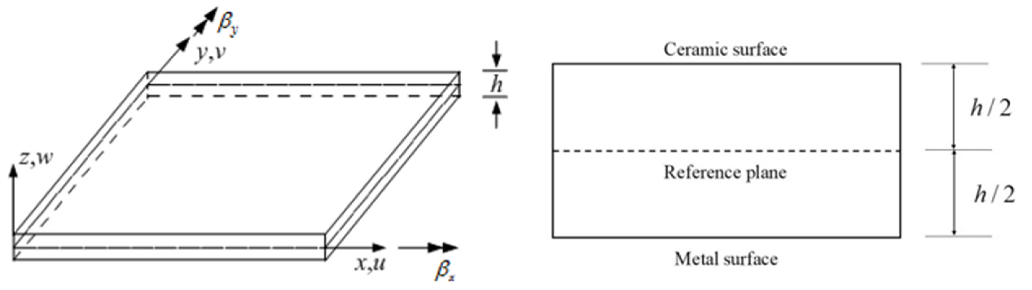
2.1. Functionally Graded Plates

A metal-ceramic FG plate of thickness h in Figure 1 is considered. The bottom and top faces of plate are assumed to be fully metal and ceramic, respectively, and the gradient property varying along z-direction. Throughout the study, the Poisson’s ratio $\nu$, Young’s modulus E, and density $\rho$ vary through the thickness as [18,40]

$$E\left(z\right)=E_m+\left(E_c-E_m\right)V_c(z)$$

(1)

$$\rho \left(z\right)={\rho }_m+\left({\rho }_c-{\rho }_m\right)V_c(z)$$

(2)

$$\nu \left(z\right)={\nu }_m+\left({\nu }_c-{\nu }_m\right)V_c(z)$$

(3)

where $V_c$ is the volume fraction of the ceramic phase, z is the thickness coordinate variable with $-h/2\le z\le h/2$, and subscripts c and m represent the ceramic and metal constituents, respectively.

2.2. NURBS Basis Functions

Before designing the volumetric fraction with any desired order continuity along the thickness, the NURBS basis functions are used in the description of the volume fraction distribution and approximation of the solutions. We give a concise introduction of the NURBS basis functions. For details on NURBS, please refer to [41].

In 1D parametric space $\xi \in \left[0,1\right]$, a knot vector $\mathit{k}\left(\xi \right)$ is a non-decreasing sequence of real numbers as

$$\mathit{k}\left(\xi \right)=\left\{{\xi }_1=0,{\xi }_2,\dots ,{\xi }_i,\dots ,{\xi }_{n+p+1}=1\right\}$$

(4)

where i is the knot index, ${\xi }_i$ is the ith knot, n is the number of basis functions, and p is the order of the polynomial. $\mathit{k}\left(\xi \right)$ is called an open knot vector when its first and last knots have multiplicity equal to p + 1. With a given knot vector, the ith B-spline basis function of degree p are defined recursively as

$$N_{i,0}=\{\begin{array}{c}1 \mathit{if}{\xi }_i\le \xi <{\xi }_{i+1}\hfill \\ 0 \mathit{otherwise}\hfill \end{array}$$

(5)

and for $p\ge 1$

$$N_{i,p}\left(\xi \right)=\frac{\xi -{\xi }_i}{{\xi }_{i+p}-{\xi }_i}{N}_{i,p-1}\left(\xi \right)+\frac{{\xi }_{i+p+1}-\xi }{{\xi }_{i+p+1}-{\xi }_{i+1}}{N}_{i+1,p-1}\left(\xi \right)$$

(6)

Note that 0/0 is defined as 0 in the evaluation.

The NURBS basis function $R_{i,p}\left(\xi \right)$ is constructed by a weighted average of the B-spline basis functions as follows

$$R_{i,p}\left(\xi \right)=\frac{N_{i,p}\left(\xi \right)w_i}{{{\displaystyle \sum }}_{j=1}^n{N}_{j,p}\left(\xi \right)w_j}$$

(7)

where $w_i$ is the ith weight, the NURBS basis function is degenerate into B-spline basis function when $w_i=1$.

The bivariate NURBS basis function for a NURBS surface is given by

$$R_{i,j}^{p,q}\left(\xi ,\eta \right)=\frac{N_{i,p}\left(\xi \right)N_{j,q}\left(\eta \right)w_{i,j}}{{{\displaystyle \sum }}_{i=1}^n{{\displaystyle \sum }}_{j=1}^m{N}_{i,p}\left(\xi \right)N_{j,q}\left(\eta \right)w_{i,j}}=\frac{N_{i,p}\left(\xi \right)N_{j,q}\left(\eta \right)w_{i,j}}{W\left(\xi ,\eta \right)}$$

(8)

where ${\mathit{w}}_{i,j}$ represents the 2D weight; $N_{j,q}(\eta )$ is the B-spline basis of order p defined on the knot vector $\mathit{k}\left(\eta \right)$, followed by recursive formulas in Equations (5) and (6); $W\left(\xi ,\eta \right)={\displaystyle \sum }_{i=1}^n{\displaystyle \sum }_{j=1}^m{N}_{i,p}\left(\xi \right)N_{j,q}\left(\eta \right)w_{i,j}$ is the weighted function for a NURBS surface.

By defining W as the diagonal matrix of weights for a NURBS surface,

$$\mathit{W}=\left[\begin{array}{cccc}{w}_1& & & \\ & w_2& & \\ & & \ddots & \\ & & & w_{n\times m}\end{array}\right]$$

(9)

and let N be the vector of B-spline basis functions, then Equation (8) can be rewritten in matrix form as

$$\mathit{R}\left(\xi ,\eta \right)=\frac{1}{W\left(\xi ,\eta \right)}\mathit{W}\mathit{N}$$

(10)

2.3. Bézier Extraction of NURBS

In order to embed the IGA program into existing FEM code, the Bézier extraction operator is adopted to construct B-spline/NURBS basis functions. The basic idea is to use Bézier decomposition to map the B-spline/NURBS basis functions over the element in the form of Bernstein polynomial basis defined on the Bézier element [26]. The B-spline/NURBS basis functions usually have $C^{p-f}$ continuous across the knots, where f is the multiplicity of the knot. With a given B-spline/NURBS curve, the continuity of the basis functions can be reduced by knot insertion and without altering the B-spline/NURBS curve. By this way, Bézier decomposition creates C⁰ Bézier elements over each knot interval. In other words, the B-spline/NURBS curve can be replaced by C⁰ Bézier curve and B-spline/NURBS basis functions will be identical to the Bernstein polynomials of order p within each element and only new control points are arisen. And the C⁰ Bézier elements are similar to the Lagrange elements straightforwardly integrating into the existing FEM code [26].

Consider $k\left(\xi \right)=\left\{{\xi }_1=0,{\xi }_2,\dots ,{\xi }_i,\dots ,{\xi }_{n+p+1}=1\right\}$ is the original knot vector, let us insert a new knot $\overline{\xi }\in [{\xi }_k,{\xi }_{k+1})\left(k>p\right)$ into the knot vector, the total number of the new basis functions and control points is then reaches m = n + 1, and the new control points ${\stackrel{-}{\mathit{P}}}_i$ can be obtained from the old control points ${\mathit{P}}_i$ according to [26,35,41]

$${\stackrel{-}{\mathit{P}}}_i=\{\begin{array}{c}{\mathit{P}}_1\hspace{1em}i=1\hfill \\ {\alpha }_i{\mathit{P}}_i+\left(1-{\alpha }_i\right)\hspace{1em}{\mathit{P}}_{i-1} 1<i<m\hfill \\ {\mathit{P}}_n\hspace{1em}i=m\hfill \end{array}$$

(11)

with

$${\alpha }_i=\{\begin{array}{c}1\hspace{1em}i\le k-p\hfill \\ \hfill \frac{\xi -{\xi }_i}{{\xi }_{i+p}-{\xi }_i}\hspace{1em}k-p+1\le i\le k\\ 0\hspace{1em}i\ge k+1\hfill \end{array}$$

(12)

It is worth noting that the same knot value may be inserted multiple times and it reduces the continuity of the basis functions by one for each insertion. But, the continuity of the curve or surface is preserved as the control variables in Equations (11) and (12) are chosen.

Based on [26,35,41], the relationship between new control points ${\overline{\mathit{P}}}^{j+1}$ and the old control points ${\overline{\mathit{P}}}^j$ (${\overline{\mathit{P}}}^1=\mathit{P}$ is the original) at the jth knot inserted can be written in matrix form

$${\overline{\mathit{P}}}^{j+1}={\left({\mathit{C}}^j\right)}^T{\overline{\mathit{P}}}^j$$

(13)

where the Bézier extraction operator of the jth knot inserted is defined by

$${\mathit{C}}^j=\left[\begin{array}{cccccc}{\alpha }_1& 1-{\alpha }_2& 0& \cdots & & 0\\ 0& {\alpha }_2& 1-{\alpha }_3& 0& \cdots & 0\\ ⋮& & & \ddots & & ⋮\\ 0& \cdots & & & {\alpha }_{n+j-1}& 1-{\alpha }_{n+j}\end{array}\right]$$

(14)

By defining $\left\{{\overline{\xi }}_1,{\overline{\xi }}_2,\cdots {\overline{\xi }}_j,\cdots ,{\overline{\xi }}_m\right\}$ as the set of inserted knots vector, the whole Bézier extraction operator is obtained as

$${\mathit{C}}^T={\left({\mathit{C}}^m\right)}^T{\left({\mathit{C}}^{m-1}\right)}^T\dots {\left({\mathit{C}}^1\right)}^T$$

(15)

With Bézier extraction, the relationship between new Bézier control points ${\mathit{P}}^b$ and original B-splines control points $\mathit{P}$ is given as

$${\mathit{P}}^b={\mathit{C}}^T\mathit{P}$$

(16)

The B-spline curve is given by

$$\mathit{X}\left(\xi \right)={\mathit{P}}^{\mathit{T}}\mathit{N}\left(\xi \right)$$

(17)

where $\mathit{N}\left(\xi \right)$ is B-spline basis function. After inserting knots, the B-spline curve with Bézier points is written as

$$\mathit{X}\left(\xi \right)={\left({\mathit{P}}^b\right)}^T\mathit{B}\left(\xi \right)={\mathit{P}}^T\mathit{C}\mathit{B}\left(\xi \right)$$

(18)

where $\mathit{B}\left(\xi \right)$ is Bernstein polynomial basis function.

Normally, it is unnecessary to establish the global extraction operator. Instead, only the local extraction operator of each element is needed. Therefore, from Equations (17) and (18), it obtains

$${\mathit{N}}^e\left(\xi \right)={\mathit{C}}^e{\mathit{B}}^e\left(\xi \right)$$

(19)

Equation (19) presents the relationship between the B-spline basis function and the Bernstein polynomials through a Bézier extraction operator ${\mathit{C}}^e$ where the superscript e denotes the element number.

Using the tensor product operator, two-dimension Bernstein polynomials ${\mathit{N}}^e\left(\xi ,\eta \right)$ can be expressed as

$${\mathit{N}}^e\left(\xi ,\eta \right)={\mathit{C}}^e\left(\xi \right)\otimes {\mathit{C}}^e\left(\eta \right){\mathit{B}}^e\left(\xi ,\eta \right)$$

(20)

where ${\mathit{C}}^e\left(\xi \right)$ and ${\mathit{C}}^e\left(\eta \right)$ are the univariate element Bézier extractors, respectively, and $\mathit{B}\left(\xi ,\eta \right)$ denote the bivariate Bernstein polynomial basis function.

Based on the Bézier extraction operator, the NURBS basis functions can be obtained

$${\mathit{R}}^e=\frac{{\mathit{W}}^e{\mathit{N}}^e}{W^e}=\frac{{\mathit{W}}^e{\mathit{C}}^e{\mathit{B}}^e}{W^e}$$

(21)

The relationship between Bézier control points ${\mathit{P}}^{b,e}$ and NURBS control points ${\mathit{P}}^e$ can be written as [26,35,41]

$${\mathit{P}}^{b,e}={\left({\mathit{W}}^{b,e}\right)}^{-1}{\left({\mathit{C}}^e\right)}^T{\mathit{W}}^e{\mathit{P}}^e$$

(22)

with ${\mathit{W}}^{b,e}$ defining the local Bézier weights, which is in diagonal matrix.

Based on Equations (10), (21) and (22), a NURBS surface is defined as

$$\mathit{X}={\mathit{P}}^T\mathit{R}={\mathit{P}}^T\frac{\mathit{W}\mathit{C}\mathit{B}}{W}=\frac{{\left({\mathit{C}}^T\mathit{W}\mathit{P}\right)}^T\mathit{B}}{W}=\frac{{\left({\mathit{W}}^b{\mathit{P}}^b\right)}^T\mathit{B}}{W}$$

(23)

Thus, based on the above equations, an NURBS curve or surface can be written equivalently in terms of a set of Bézier elements through Bézier extraction operator.

2.4. Isogeometric Analysis Mindlin Plate Formulation

Based on the Reissner–Mindlin theory, the displacements u, v, and w at a point $(x,y,z)$ in the plate, see Figure 1, are expressed as [36,40]

$$\begin{gathered} u\left(x,y,z\right)=u_0\left(x,y\right)+z{\beta }_x\left(x,y\right) \\ v\left(x,y,z\right)=v_0\left(x,y\right)+z{\beta }_y\left(x,y\right) \\ w\left(x,y,z\right)=w_0\left(x,y\right) \end{gathered}$$

(24)

where $u_0$, $v_0$, $w_0$ are the reference plane displacements components in the x, y, and z axis, respectively. ${\beta }_x$ and ${\beta }_y$ are the transverse normal rotations in the xz- and yz-planes of reference plane.

By making the usual small strain assumptions, the strain–displacement relations are expressed in the following matrix form

$$\mathit{\epsilon }=\left\{\begin{array}{c}{\mathit{\epsilon }}_p\\ \mathit{0}\end{array}\right\}+\left\{\begin{array}{c}z{\mathit{\epsilon }}_b\\ {\mathit{\epsilon }}_s\end{array}\right\}$$

(25)

The reference plane strains ${\mathit{\epsilon }}_p$, the bending strains ${\mathit{\epsilon }}_b$, and the shear strain ${\mathit{\epsilon }}_s$ in Equation (25) are written as

$${\mathit{\epsilon }}_p=\left\{\begin{array}{c}{u}_{0,x}\\ v_{0,y}\\ u_{0,y}+v_{0,x}\end{array}\right\},{\mathit{\epsilon }}_b=\left\{\begin{array}{c}{\beta }_{x,x}\\ {\beta }_{y,y}\\ {\beta }_{x,y}+{\beta }_{y,x}\end{array}\right\},{\mathit{\epsilon }}_s=\left\{\begin{array}{c}{\beta }_x+w_{0,x}\\ {\beta }_y+w_{0,y}\end{array}\right\}$$

(26)

where the subscript comma denotes the partial derivative with respect to the spatial coordinate succeeding it. The constitutive relations are derived from Hook’s law as

$$\mathit{\sigma }={\mathit{D}}_m\left(z\right)\left({\mathit{\epsilon }}_p-z{\mathit{\epsilon }}_b\right),\mathit{\tau }={\mathit{D}}_s\left(z\right)\mathit{\gamma }$$

(27)

where $\mathit{\sigma }=[\begin{array}{ccc}{\mathit{\sigma }}_x& {\mathit{\sigma }}_y& {\mathit{\tau }}_{xy}\end{array}]$, $\mathit{\tau }=[\begin{array}{cc}{\mathit{\tau }}_{xz}& {\mathit{\tau }}_{yz}\end{array}]$ are the in-plane stress and shear stress respectively, and material matrices ${\mathit{D}}_m(z)$ and ${\mathit{D}}_s(z)$ are given as

$${\mathit{D}}_m\left(z\right)=\frac{E\left(z\right)}{1-v{(z)}^2}\left[\begin{array}{ccc}1& v\left(z\right)& 0\\ v\left(z\right)& 1& 0\\ 0& 0& \frac{1-v\left(z\right)}{2}\end{array}\right],{\mathit{D}}_s\left(z\right)=\frac{1}{2}\frac{\alpha E\left(z\right)}{1+v\left(z\right)}\left[\begin{array}{cc}1& 0\\ 0& 1\end{array}\right]$$

(28)

where $\alpha$ is the shear correction factor, and $\alpha$ = 5/6 is adopted in this study for simplicity [40].

In the parametric domain in the IGA framework, the finite element approximation uses NURBS basis function. Thus, the generalized displacements in the reference plane are approximated as follows

$${\mathit{u}}_0^h={{\displaystyle \sum }}_{I=1}^{NP}{R}_I{\mathit{u}}_I$$

(29)

with

$${\mathit{u}}_0^h={\left[\begin{array}{ccccc}{u}_0^h& v_0^h& w^h& {\beta }_x& {\beta }_y\end{array}\right]}^T$$

(30)

$${\mathit{u}}_I={\left[\begin{array}{ccccc}{u}_I& v_I& w_I& {\beta }_{Ix}& {\beta }_{Iy}\end{array}\right]}^T$$

(31)

where NP = (p + 1) (q + 1) is the number of the control points per element, and R_I and u_I denote the shape function and the unknown displacement vector at Ith control point, respectively.

By substituting Equation (29) to (26), and we obtained

$${\mathit{\epsilon }}_p={{\displaystyle \sum }}_{I=1}^{NP}{\mathit{B}}_I^p{\mathit{u}}_I,{\mathit{\epsilon }}_b={{\displaystyle \sum }}_{I=1}^{NP}{\mathit{B}}_I^b{\mathit{u}}_I,\mathit{\gamma }={{\displaystyle \sum }}_{I=1}^{NP}{\mathit{B}}_I^s{\mathit{u}}_I$$

(32)

with

$${\mathit{B}}_I^p=\left[\begin{array}{ccccc}{R}_{I,x}& 0& 0& 0& 0\\ 0& R_{I,y}& 0& 0& 0\\ R_{I,y}& R_{I,x}& 0& 0& 0\end{array}\right],{\mathit{B}}_I^b=\left[\begin{array}{ccccc}0& 0& 0& R_{I,x}& 0\\ 0& 0& 0& 0& R_{I,y}\\ 0& 0& 0& R_{I,y}& R_{I,x}\end{array}\right],{\mathit{B}}_I^s=\left[\begin{array}{ccccc}0& 0& R_{I,x}& R_I& 0\\ 0& 0& R_{I,y}& 0& R_I\end{array}\right]$$

(33)

For free vibration analysis, a weak form can be established as

$${{\displaystyle \int }}_{\Omega }\delta {\mathit{\epsilon }}^T\mathit{D}\mathit{\epsilon }d\Omega +{{\displaystyle \int }}_{\Omega }\delta {\mathit{\gamma }}^T{\mathit{D}}^s\mathit{\gamma }d\Omega ={{\displaystyle \int }}_{\Omega }\delta {\mathit{u}}^T\mathit{m}\ddot{\mathit{u}}d\Omega$$

(34)

where

$$\mathit{\epsilon }=\left[\begin{array}{c}{\mathit{\epsilon }}_p\\ {\mathit{\epsilon }}_b\end{array}\right],\mathit{D}=\left[\begin{array}{cc}{\mathit{D}}^m& \overline{\mathit{B}}\\ \overline{\mathit{B}}& {\mathit{D}}^b\end{array}\right],{\mathit{D}}^s={{\displaystyle \int }}_{-h/2}^{h/2}{\mathit{D}}_s\left(z\right)dz$$

(35)

$${\mathit{D}}^m={{\displaystyle \int }}_{-h/2}^{h/2}{\mathit{D}}_m\left(z\right)dz,\overline{\mathit{B}}={{\displaystyle \int }}_{-h/2}^{h/2}z{\mathit{D}}_m\left(z\right)dz,{\mathit{D}}^b={{\displaystyle \int }}_{-h/2}^{h/2}{z}^2{\mathit{D}}_m\left(z\right)dz$$

(36)

$$m=\left[\begin{array}{ccccc}{I}_0& 0& 0& I_1& 0\\ 0& I_0& 0& 0& I_1\\ 0& 0& I_0& 0& 0\\ I_1& 0& 0& I_2& 0\\ 0& I_1& 0& 0& I_2\end{array}\right],\left(I_0,I_1,I_2\right)={{\displaystyle \int }}_{-h/2}^{h/2}\rho \left(z\right)\left(1,z,z^2\right)dz$$

(37)

By taking Equations (29)–(33) into (34), the formulation of the free vibration is recast as

$$\left(\mathit{K}-{\omega }^2\mathit{M}\right)\mathit{u}=0$$

(38)

where

$$\mathit{K}={{\displaystyle \int }}_{\Omega }{\left\{\begin{array}{c}{\mathit{B}}^p\\ {\mathit{B}}^b\end{array}\right\}}^T\left[\begin{array}{cc}{\mathit{D}}^m& \overline{\mathit{B}}\\ \overline{\mathit{B}}& {\mathit{D}}^b\end{array}\right]\left\{\begin{array}{c}{\mathit{B}}^p\\ {\mathit{B}}^b\end{array}\right\}d\Omega +{{\displaystyle \int }}_{\Omega }{\left({\mathit{B}}^s\right)}^T{\mathit{D}}^s{\mathit{B}}^{s}d\Omega$$

(39)

$$\mathit{M}={{\displaystyle \int }}_{\Omega }{\mathit{N}}^T\mathit{m}\mathit{N}d\Omega$$

(40)

$${\mathit{N}}_I=\left[\begin{array}{ccccc}{R}_I& 0& 0& 0& 0\\ 0& R_I& 0& 0& 0\\ 0& 0& R_I& 0& 0\\ 0& 0& 0& R_I& 0\\ 0& 0& 0& 0& R_I\end{array}\right]$$

(41)

where $\omega$ is the natural frequency.

3. Volume Fraction Optimization by Particle Swarm Optimization

3.1. Formulation of the Optimization Problem

The material distribution can be optimized by designing the volume fractions profile via the volume fraction of the control points. A constrained optimization problem is established as

$$\begin{array}{cc}\mathrm{Find}\hfill & V_i,i=1,2,\dots ,N\hfill \\ \mathrm{Minimize}\hfill & f\left(V_i\right)\hfill \\ \mathrm{Subject}\mathrm{to}\hfill & g_j\left(V_i\right)\le 0,j=1,2,\cdots ,J\hfill \\ & h_k\left(V_i\right)=0,k=1,2,\cdots ,K\hfill \\ & \hfill 0\le V_i\le 1\hfill \end{array}$$

(42)

where $V_i$ is the volume fractions of the ceramic on the ith control points. N is the number of the control points. $f(V_i,{\omega }_i)$ is the objective function, $g_j(V_i,{\omega }_i)$ is the jth inequality constraint, and $h_k(V_i,{\omega }_i)$ is the kth equality constraint. $0\le V_i\le 1$ is the physical bound for the volume fraction. The specific forms of the objective function and constraint will be detailed in the numerical experiments.

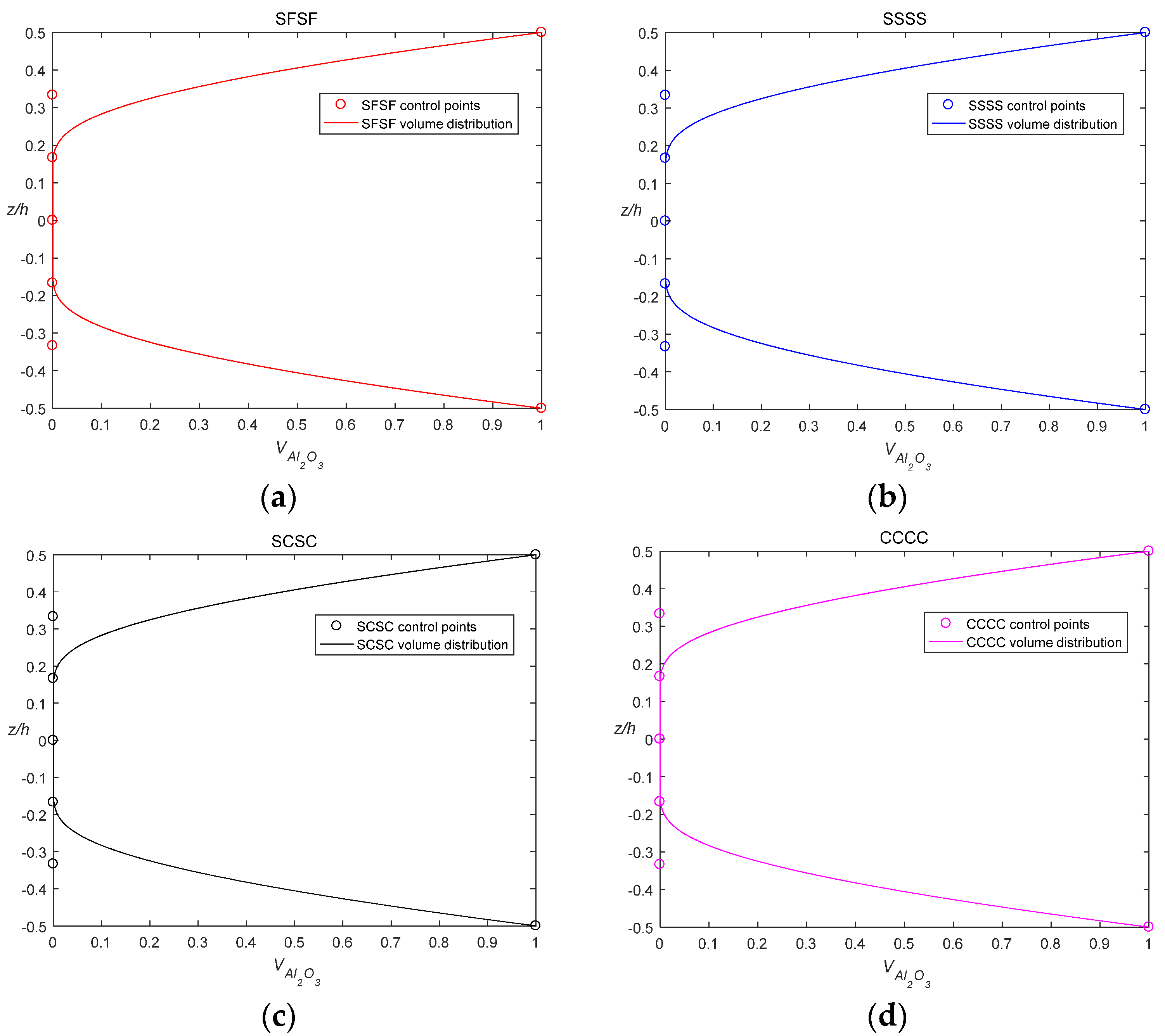
3.2. Volume Fraction Distribution Parameterization

In this study, the volume fraction is obtained as a NURBS curve with a weighted linear combination of the NURBS basis functions as

$$V\left(u\right)={\displaystyle \sum }_{i=0}^N{R}_{i,p}\left(u\right)V_i, 0\le V\le 1$$

(43)

where $V_i$ is the volume fraction of the control points to generate the volume fraction curve. The NURBS can represent complex shapes with a few control points. This property makes the NURBS curves promising to achieve a more complex desired profile of the material distribution by determining control points. The control weights of the material profile are set to one, so the NURBS basis function is degenerated into B-spline basis function for the volume fraction description.

With the proposed Equation (43), it is easy to restrict the volume fraction within the physical upper and lower bounds; namely, $0\le V(u)\le 1$ by setting design variables $V_i$ in the interval [0, 1]. This advantage results from the strong convex hull property that the curve is contained in the convex hull of its control polygon [41]. Thus, it is convenient to apply the physical constraints without any extra computations. Furthermore, it is easy to access any desired order continuity with selecting the degree p of the basis function. The continuity of the volumetric profile across the control points is determined by the continuity of the basis across the knot span. Nevertheless, more control points are required for higher order continuity. In this study, p = 3 is selected. In principle, the present technique circumvents the difficulties of existing methods in the volume fraction description.

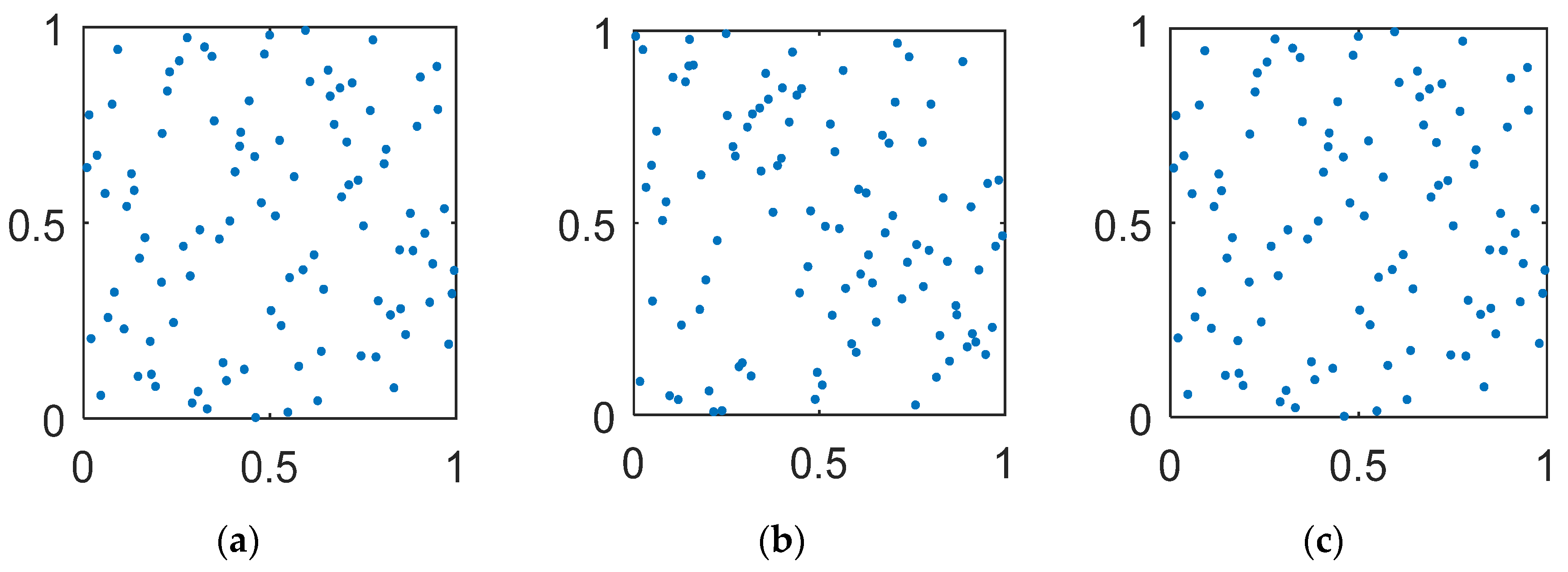
3.3. Particle Swarm Optimization

Classical gradient-based algorithms compute the sensitivity of the objective functions to enhance their performance in searching for optimal solutions. Nevertheless, it may encounter the difficulty of getting stuck in a local optimum for non-convex problems. Sufficiently smooth is required to guarantee the existence of its first (and often second) derivatives. Metaheuristic algorithms are ideal candidates at finding global solutions in the complexity and non-convex problems. In this study, we employ PSO.

PSO is a population approach with stochastic perturbations, which is developed by Kennedy and Eberhart [42]. It is inspired by the movement of natural swarms and flocks such as fish and bird schooling in nature. The PSO is becoming powerful and increasingly popular.

In the PSO, the design variables are set as the coordinates x to describe the spatial position in the search space, and thus a group of the design variables are considered as an N-dimensional particle. In the beginning, a number of entities are placed in the search space. The objective function at the current location is evaluated at each particle. Then the particle is attracted to the current global best location and its own best location in the history. At the same time, the movement is stochastically oscillated on the way to the best locations. The particle’s location is iteratively updated until converged. The particle swarm optimization contains the following steps:

• Initialized population (t = 0), 100 in this study, of particles with random positions ${\overrightarrow{x}}_i^0$ and velocities ${\overrightarrow{v}}_i^0$ in the search space;
• Evaluate the objective function for each particle, and compare the particle’s fitness function to obtain the global best fitness and its location $\overrightarrow{p}$, and identify the best location $\overrightarrow{g}$ in the neighborhood;
• Update the velocity and position of the particle according to

  $$\{\begin{array}{l}{\overrightarrow{v}}_i^{t+1}=w{\overrightarrow{v}}_i^t+\alpha {\overrightarrow{u}}_1\odot (\overrightarrow{p}-{\overrightarrow{x}}_i^t)+\beta {\overrightarrow{u}}_2\odot (\overrightarrow{g}-{\overrightarrow{x}}_i^t)\\ {\overrightarrow{x}}_i^{t+1}={\overrightarrow{x}}_i^t+{\overrightarrow{v}}_i^{t+1}\end{array}$$

  where w is inertia weight, and is set as 0.9, $\alpha ,\beta$ are adjustment weights, set as 1.49 [42] ${\overrightarrow{u}}_1,{\overrightarrow{u}}_2$ are two random vectors, and each entry taking the values between 0 and 1. $\odot$ is the entry-wise product, that is ${\left[a\odot b\right]}_{ij}=a_{ij}{b}_{ij}$.
• Enforce the bounds. If any component of x is outside a bound, set it equal to that bound.
• Set t = t + 1, and repeat steps 2–4 until either a maximum number of generations has been achieved, or a satisfactory convergence has been reached for the population.

The selection of initial population is important to achieve fast convergence and to prevent local minima. It is essential to allocate the initial particles to fill the design space. One of the most popular techniques for uniform distribution is a Latin hypercube design. It is inspected to possess the highest overall sparseness. The distribution is improved by maximizing the minimum distance between points (Figure 2).

The penalty function method is involved to handle the constraints. In this method, problem (42) is reconstructed as

$$\begin{array}{cc}\mathrm{Find}\hfill & V_i,i=1,2,\dots ,N\hfill \\ \mathrm{Minimize}& f(V_i)+c\left({\displaystyle \sum _{j=1:J}\max (0,g_j(V_i))}+{\displaystyle \sum _{k=1:K}\left|h_k(V_i)\right|}\right)\hfill \end{array}$$

(44)

c is the penalty parameter. In this work, c is selected as 100.

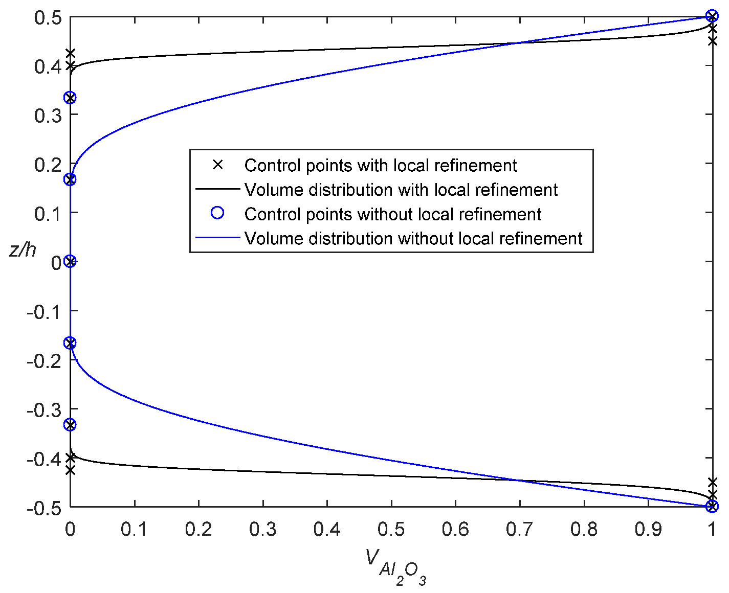
3.4. Local Refinement for Graded Regions

It is possible to yield the laminate-like results after the optimization. Between the constitutional materials, there is a graded region where one material smoothly transits to another in the FGMs. The thickness of the transition zone may influence optimal results. Therefore, we develop a strategy to identify the graded region. The following steps are proposed:

• Define a sparse knot vector for the control points and initialize their volume fractions;
• Optimize the volume fraction with the PSO;
• Refine the optimal results:
  • (a) If $\left|V_i-V_{i+1}\right|>0.9$, then insert four data points for volume fraction description between $\left(z_i,V_i\right)$ and $\left(z_{i+1},V_{i+1}\right)$, i.e., $\left(z_i+\delta ,V_i\right)$, $\left(z_i+\delta +d,V_i\right)$, $\left(z_i+\delta +2d,V_{i+1}\right)$ and $\left(z_i+\delta +3d,V_{i+1}\right)$, where $\delta$ and $d$ are used to describe the location and the thickness of the transition zone;
  • (b) If $\left|V_i-V_{i+1}\right|<0.9$ and $\left|V_{i+1}-V_{i+2}\right|<0.9$ and $\left|V_i-V_{i+2}\right|>0.9$, then delta data $\left(z_{i+1},V_{i+1}\right)$ and insert four points between $\left(z_i,V_i\right)$ and $\left(z_{i+2},V_{i+2}\right)$, i.e., $\left(z_i+\delta ,V_i\right)$, $\left(z_i+\delta +d,V_i\right)$, $\left(z_i+\delta +2d,V_{i+2}\right)$ and $\left(z_i+\delta +3d,V_{i+2}\right)$;
• Optimize parameters $\delta$ and $d$ to update the volume fraction curves until converged.

A detailed numerical description of this method can be found in Section 4.3.

4. Results and Discussions

In this section, some examples are employed to illustrate the feasibility of the present method in the design of the FG plate in the free vibration problem.

A FG square plate is considered for all cases in Figure 1. The dimensions of the plate are a = b = 1 m. The FG plate is made up of metal (Al) and ceramic (Al₂O₃). The material properties of the constituents are given in

Table 1. Material properties for Al and Al₂O₃ [43].

Material Property	Al	Al2O3
E(GPa)	70	380
$\nu$ $\rho$ (kg/m3)	0.3 2707	0.25 3800

. The natural frequency involved in this study is obtained with the IGA simulation by the Bézier extraction of NURBS, based on the Mindlin theory. The plane is modeled by a net of 18 × 18 control points and 15 × 15 elements by using the cubic NURBS basis function in Figure 3. All dimensionless frequencies are defined by ${\omega }^{*}=\omega {\pi }^2\left(a^2/h\right)\sqrt{{\rho }_m/E_m}$.

In the following examples, the constraint boundaries are obtained by the Mindlin theory with the power-law FG plate. The volume fraction $V_c$ of the ceramic in the FG plate with the power-law distribution is

$$V_c={\left(\frac{z}{h}+\frac{1}{2}\right)}^n$$

(45)

where n is the volume fraction exponent, also known as the gradient index. Thus, the volume fraction of metal $V_m$ is $V_m=1-V_c$. In optimization problems, volumetric fractions are parameterized by Equation (43) with cubic NURBS where control weights are set to one.

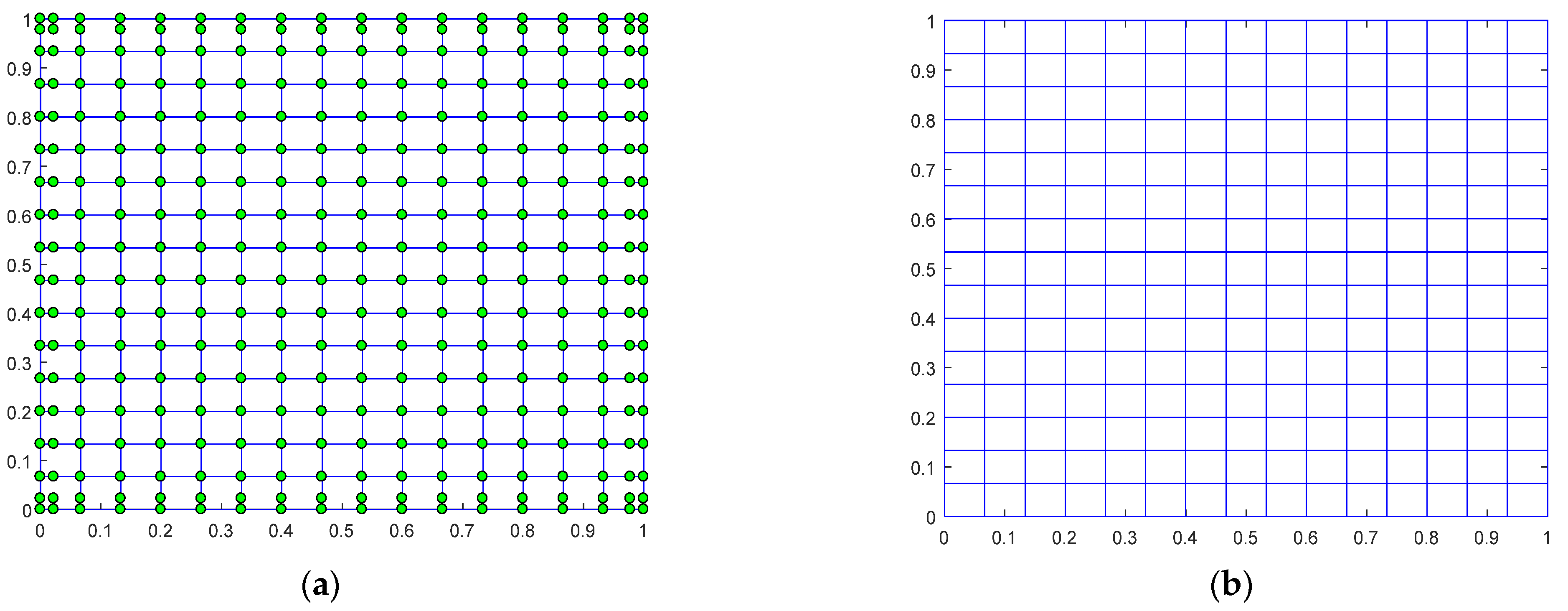
4.1. IGA Simulation by Bézier Extraction of NURBS

The accuracy of the IGA simulation by the Bézier extraction of NURBS is investigated via an Al/Al₂O₃ square thin plate with a length–thickness ratio of a/h = 100 under different boundary conditions and gradient indices are considered.

Table 2. First five normalized natural frequencies of Al/Al₂O₃ thin plate with various boundary conditions and gradient indices.

n	Method	Mode 1	Mode 2	Mode 3	Mode 4	Mode 5
(a) SFSF
0	IGA with Bézier extraction of NURBS	56.5512	94.6494	215.3262	228.5588	274.1382
	S-FSDT-based IGA [40]	56.5584	94.7388	215.5711	228.5829	274.2876
	Zienkiewicz [44]	56.4791	94.7141	215.6299	-	-
0.5	IGA with Bézier extraction of NURBS	47.8860	80.1536	182.3564	193.5485	232.1575
	S-FSDT-based IGA [40]	47.8913	80.2210	182.5386	193.5617	232.2649
	Zienkiewicz [44]	47.7452	80.1576	182.4411	-	-
1	IGA with Bézier extraction of NURBS	43.1501	72.2290	164.329	174.4098	209.205
	S-FSDT-based IGA [40]	43.1544	72.2861	164.4815	174.4179	209.2924
	Zienkiewicz [44]	43.0872	72.2001	164.3911	-	-
2	IGA with Bézier extraction of NURBS	39.2307	65.6675	149.3978	158.565	190.1972
	S-FSDT-based IGA [40]	39.2347	65.7197	149.5365	158.5722	190.2767
	Zienkiewicz [44]	39.1666	65.6400	149.0583	-	-
(b) SSSS
0	IGA with Bézier extraction of NURBS	115.8928	289.59	289.59	463.0858	578.8734
	S-FSDT-based IGA [40]	115.8926	289.5806	289.5806	463.0741	578.7215
	Zienkiewicz [44]	115.8695	289.7708	-	463.4781	-
0.5	IGA with Bézier extraction of NURBS	98.1350	245.23	245.23	392.1661	490.2589
	S-FSDT-based IGA [40]	98.1343	245.2169	245.2169	392.1448	490.0963
	Zienkiewicz [44]	98.0136	245.3251	-	392.4425	-
1	IGA with Bézier extraction of NURBS	88.4292	220.9798	220.9798	353.3897	441.7981
	S-FSDT-based IGA [40]	88.428	220.9643	220.9643	353.3613	441.6348
	Zienkiewicz [44]	88.3093	221.0643	-	353.6252	-
2	IGA with Bézier extraction of NURBS	80.3968	200.9035	200.9035	321.2784	401.6464
	S-FSDT-based IGA [40]	80.3953	200.8879	200.8879	321.2475	401.5008
	Zienkiewicz [44]	80.3517	200.8793	-	321.4069	-
(c) SCSC
0	IGA with Bézier extraction of NURBS	169.8842	321.1324	406.4732	554.2942	599.3743
	S-FSDT-based IGA [40]	169.9230	321.1937	406.5707	554.5021	599.3170
	Zienkiewicz [44]	170.0196	321.4069	-	555.2809	-
0.5	IGA with Bézier extraction of NURBS	143.8626	271.9523	344.2506	469.4564	507.6351
	S-FSDT-based IGA [40]	143.8904	271.9916	344.3090	469.5928	507.5430
	Zienkiewicz [44]	143.8179	272.1090	-	470.0770	-
1	IGA with Bézier extraction of NURBS	129.6378	245.0642	310.2251	423.0577	457.4619
	S-FSDT-based IGA [40]	129.6605	245.0927	310.2664	423.1599	457.3585
	Zienkiewicz [44]	129.6496	245.1310	-	423.6904	-
2	IGA with Bézier extraction of NURBS	117.8613	222.7987	282.0365	384.6108	415.8853
	S-FSDT-based IGA [40]	117.8818	222.8238	282.0750	384.7018	415.7952
	Zienkiewicz [44]	117.8104	222.8111	-	385.0672	-
(d) CCCC
0	IGA with Bézier extraction of NURBS	211.1102	430.2397	430.2397	633.8258	770.8743
	S-FSDT-based IGA [40]	211.1468	430.3633	430.3633	634.1625	770.8950
	Difference	0.0173%	0.0287%	0.0287%	0.0531%	0.0027%
0.5	IGA with Bézier extraction of NURBS	178.7791	364.3864	364.3864	536.8548	653.0164
	S-FSDT-based IGA [40]	178.8047	364.4639	364.4639	537.0816	652.9193
	Difference	0.0143%	0.0213%	0.0213%	0.0422%	0.0149%
1	IGA with Bézier extraction of NURBS	161.1039	328.3736	328.3736	483.8103	588.5278
	S-FSDT-based IGA [40]	161.1242	328.4308	328.4308	483.9866	588.3962
	Difference	0.0126%	0.0174%	0.0174%	0.0364%	0.0224%
2	IGA with Bézier extraction of NURBS	146.4685	298.5351	298.5351	439.8380	535.0256
	S-FSDT-based IGA [40]	146.4868	298.5884	298.5884	439.9988	534.9293
	Difference	0.0125%	0.0179%	0.0179%	0.0365%	0.0180%

compares the first five mode normalized natural frequencies obtained with different methods. The results obtained based on the FSDT via different methods are in good agreement with each other. If fewer constraints are added to the boundary, changing from CCCC to SCSC, SSSS, and SFSF, the natural frequency gradually decreases. The magnitude of the natural frequency decreases with an increasing gradient index. It can be explained by the fact that as the gradient index increases, the volume fraction of the ceramic is lower, and the plate has a lower stiffness. It should be noted that the IGA with the Bézier extraction of NURBS by using the cubic NURBS basis function eliminates the shear locking phenomena in the thin plate.

It is obvious that the distribution of the volumetric fraction will influence the natural frequency of an FG plate. In the following part, the volumetric fraction distribution will be optimized to explore the dynamic performance of an FG plate, where the volumetric fraction is parameterized by Equation (43) with control weights of the material profile set to one.

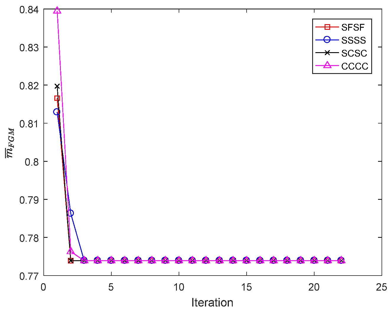
4.2. Maximize the Difference between Consecutive Frequencies

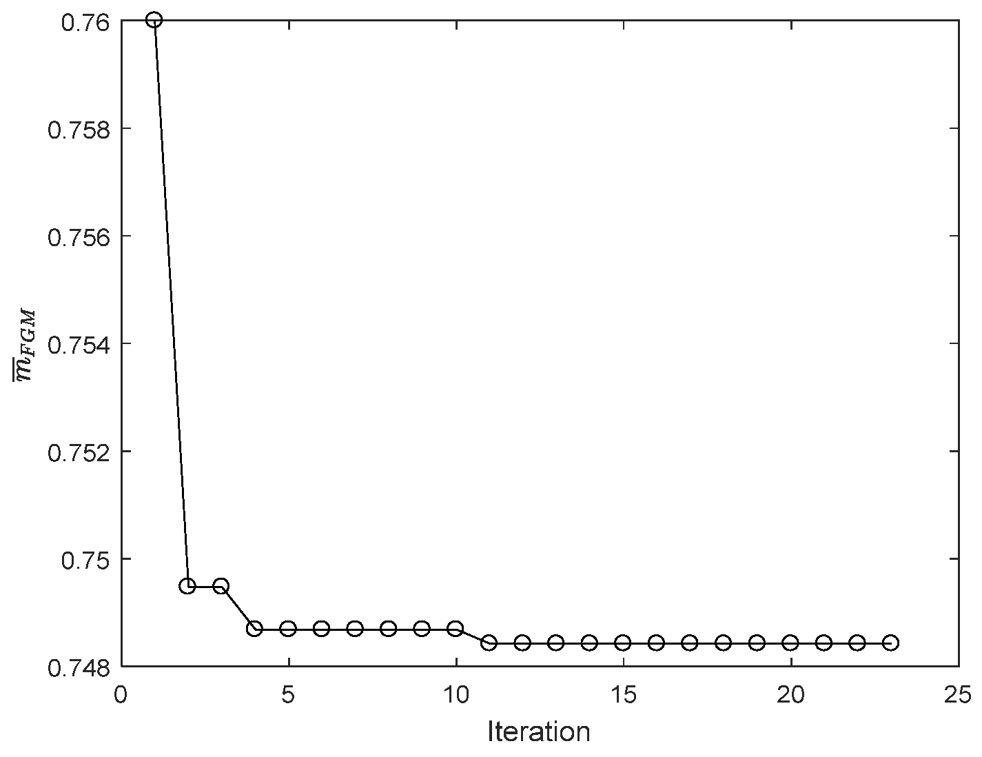
In order to avoid the resonance in a certain frequency band, it is required to increase the difference of two consecutive frequencies. In this section, we consider a natural frequency optimization problem to maximize the frequency distance between the first two natural frequencies of the plate.

A simply supported FGM square plate is considered. The length–thickness ratio is a/h = 20. Both top and bottom surfaces are ceramic. Eleven evenly distributed control points are located in the thickness direction to define the volume fraction $V_c$ of the ceramic by Equation (43). Then the optimization problem is stated as

$$\begin{array}{cc}\mathrm{Find}\hfill & V_i,i=2,3,\dots ,10\hfill \\ \mathrm{minimize}\hfill & f(V_i)={\omega }_1^{*}-{\omega }_2^{*}\hfill \\ \mathrm{Subject}\mathrm{to}\hfill & g_1=\frac{{\displaystyle {\int }_{-h/2}^{h/2}\left[{\rho }_c{V}_c+{\rho }_m\left(1-V_c\right)\right]dz}}{h{\rho }_c}-{\overline{m}}_0\le 0\hfill \\ & 0\le V_i\le 1,V_1=1,V_{11}=1.\hfill \end{array}$$

(46)

where the constraint boundary ${\overline{m}}_0=\frac{{\displaystyle {\int }_{-h/2}^{h/2}\left[{\rho }_c{V}_c+{\rho }_m\left(1-V_c\right)\right]dz}}{h{\rho }_c}$ is the dimensionless mass obtained from the power-law FG plate with different power-law indices as shown in

Table 3. The frequency for the simply supported FGM plate with a/h = 20.

Power-Law Index (n)	${\overline{\mathit{m}}}_0$	${\mathit{\omega }}_{\mathit{r}1}^{*}$	${\mathit{\omega }}_{\mathit{r}2}^{*}$	${\mathit{\omega }}_{\mathit{r}2}^{*}-{\mathit{\omega }}_{\mathit{r}1}^{*}$
1	0.8562	87.75	216.80	129.05
2 5	0.8082 0.7603	79.76 75.52	196.98 186.17	117.22 110.65

. The first two natural frequencies of the power-law FG plate ${\omega }_{r1}^{*},{\omega }_{r2}^{*}$ are listed in Table 3 as a reference to illustrate the effectiveness of the optimization process.

In this case, three optimization algorithms, that is the PSO, the genetic algorithm (GA), and the pattern search algorithm (PS), are performed to address this problem. The GA imitates the evolution of a creature and is based on the mechanism of natural genetics, which combines a ‘survival of the fittest’ mentality with a structured, yet random, exchange of information in order to explore the search space. The PS starts with a base point, and evaluates the objective function in a stencil-based fashion determined by a set of directions to search a descent direction until converged. The swarm size of 100 is used in the PSO. The population size of the GA is 100, as is the PSO. The tolerance of mesh size in the PS is 1 × 10⁻⁶.

The computed optimal results of the PS, GA, and PSO are tabulated in

Table 4. Optimal results of GA, PSO, and PS.

		PSO			GA			PS
n	${\mathit{\omega }}_1^{*}$	${\mathit{\omega }}_2^{*}$	${\mathit{\omega }}_2^{*}-{\mathit{\omega }}_1^{*}$	${\mathit{\omega }}_1^{*}$	${\mathit{\omega }}_2^{*}$	${\mathit{\omega }}_2^{*}-{\mathit{\omega }}_1^{*}$	${\mathit{\omega }}_1^{*}$	${\mathit{\omega }}_2^{*}$	${\mathit{\omega }}_2^{*}-{\mathit{\omega }}_1^{*}$
1	115.80	284.33	168.52	115.51	283.64	168.12	110.81	272.42	161.61
2 5	108.45 92.64	265.98 227.31	157.53 134.67	106.90 91.66	262.30 224.99	155.40 133.32	101.26 90.42	248.88 222.05	147.62 131.63

, where ${\omega }_1^{*}$ and ${\omega }_2^{*}$ are the first two natural frequencies of the optimal FG plate. The iteration history of the objective function is demonstrated in Figure 4. It should be noticed that the first several iterations are ignored for the reason that the value of the reconstructed objective function from Equation (44) is larger than 0. From Table 4 and Figure 5, it is observed that the PSO and GA offer better results, and the PS is getting stuck in the local optimum and cannot improve the results. On the other side, the PSO converges in less than 45 iterations, much less than the GA in more than 180 iterations and the PSO in more than 100 iterations. It can be observed that the GA fails to converge in 200 iterations for n = 2 and 5. Since the difference of the constraint boundary, the numbers of iterations are different for three optimization algorithms. The PS cannot obtain the best solution, and the PSO and the GA with the same population size consume the same CPU time in each iteration. We conclude that the PSO performs best among the three algorithms.

The volume distributions and control points of the optimal results along the thickness are plotted in Figure 5. From Figure 5, most of the volume fractions on the control points are on the constraint boundary in the PSO results. The optimized plate are sandwich-like plates with two transition zones at the top and bottom surface, in which the material distribution is symmetric with respect to the reference plane of the plate. The stiffer and heavier phase is mainly distributed in the vicinity of the surface of the plate, while most of the part is metal in the region near the reference plane. As the constraint dimensionless mass is lighter, the transition region is thinner. Furthermore, the difference of the first two natural frequencies of the optimized FG plate is 30% more than that of the corresponding difference of the power-law FG plate, except the result with n = 5, which is only 21% more.

Notwithstanding with the same fraction of the materials, it is promising to improve the dynamic performance of the composites by designing its material distribution. We validate the feasibility of the proposed method, and the PSO produces the best results among the three algorithms. Nevertheless, it is observed that there are two graded regions in the optimized volumetric fraction distributions, which are determined by the distance of the adjacent control points. If we can further refine the transition zone, better results may be obtained.

4.3. Minimize Mass

The mass of the plate is minimized with the frequency constrained. Both top and bottom surfaces are ceramic. The length–thickness ratio a/h = 20, and 7 evenly distributed control points are located in the thickness direction to define the volume fraction. Different boundary conditions are investigated. The optimization problem is stated as

$$\begin{array}{cc}\mathrm{Find}\hfill & V_i,i=2,\dots ,6\hfill \\ \mathrm{minimize}\hfill & \overline{m}(V_i)=\frac{{\displaystyle {\int }_{-h/2}^{h/2}\left[{\rho }_c{V}_c+{\rho }_m\left(1-V_c\right)\right]dz}}{h{\rho }_c}\hfill \\ \mathrm{Subject}\mathrm{to}\hfill & g_1={\omega }_r^{*}-{\omega }^{*}\le 0\hfill \\ & 0\le V_i\le 1,V_1=1;V_7=1\hfill \end{array}$$

(47)

where the constraint ${\omega }_r^{*}$ is the fundamental frequency of the power-law FG plate with power-law index n = 1 under different boundary conditions and listed in

Table 5. The frequency of the power-law (n = 1) and optimum FG plates under different boundary conditions.

B.C.	${\mathit{\omega }}_{\mathit{r}}^{*}$	${\overline{\mathit{m}}}_{\mathit{p}\mathit{FGM}}$	${\overline{\mathit{m}}}_{\mathit{FGM}}$	Mass Decrease
SFSF	42.94	0.8562	0.7739	9.61%
SSSS SCSC CCCC	87.75 127.24 157.35	0.8562 0.8562 0.8562	0.7739 0.7739 0.7739	9.61% 9.61% 9.61%

. The fundamental frequency of the optimal FGM should be more than the reference fundamental frequency ${\omega }_r^{*}$ as shown in $g_1$. In Table 5, ${\overline{m}}_{\mathit{pFGM}}$ and ${\overline{m}}_{\mathit{FGM}}$ are the dimensionless mass of the power-law (n = 1) and the optimum FG plates, respectively. It should be noted that the dimensionless mass of the monolithic metal is $\raisebox{1ex}{${\rho }_m$}\!\left/ \!\raisebox{-1ex}{${\rho }_c$}\right.=0.7124$. The dimensionless mass of power-law FG plate is ${\overline{m}}_{\mathit{pFGM}}=\raisebox{1ex}{${\rho }_c+{\rho }_m$}\!\left/ \!\raisebox{-1ex}{$2{\rho }_c$}\right.=0.8562$. Thus, the dimensionless mass of the optimal FG plate is bounded by (0.7124, 0.8562). It is worth noting that the maximum difference of the upper and lower bound is merely 20%.

The optimal results and volume fraction distributions are given in Table 5 and Figure 6, respectively. Figure 7 displays the iteration history. It is interesting to note that the optimal results with respect to different boundary conditions are identical. The optimal control points are distributed on the constrained boundary. The objective function is to minimize the mass of the plate, theoretically speaking that is, to reduce the volumetric fraction of the ceramic phase. Most of the FG plate consists of the lighter and slender phase, metal, mainly distributed near the reference plane, while the heavier and stiffer phase, ceramic, is in the graded regions near the top and bottom surfaces. The dimensionless mass of the optimized FG plate is around 0.7739, 9.61% lighter than the power-law FGM plate. The constituents near the top and bottom play a predominant role in the determination of the natural frequency of the FG plate.

There are two transition zones near the top and bottom surfaces. The width of the transition zone is determined by the distance of the adjacent pre-set control points. It is not applicable if the width is smaller than the distance but to uniformly refine the number of the control points. The rising number of design variables will bring more computational costs.

To efficiently determine the local graded region, we devise a local refinement strategy. Thanks to the constituent volume distributions for different boundary conditions that are in coincidence with each other, we choose a clamped plate to illustrate the strategy.

As shown in Figure 6, the transition zones lie between the first and last two control points. We, respectively, insert four control points in the regions (−h/2, −h/3) and (h/3, h/2) with four new parameters ${\delta }_1$, $d_1$, ${\delta }_2$, and $d_2$, for example, $\left(-h/2+{\delta }_1,1\right)$,$\left(-h/2+{\delta }_1+d_1,1\right)$, $\left(-h/2+{\delta }_1+2d_1,1\right)$, and $\left(-5h/12+{\delta }_1+3d_1,1\right)$ in region [−h/2, −h/3]. Then we establish another optimization problem as:

$$\begin{array}{ll}\mathrm{Find}\hfill & {\delta }_i,d_i,i=1,2\hfill \\ \mathrm{minimize}\hfill & \overline{m}(V_c\left({\delta }_i,d_i\right))=\frac{{\displaystyle {\int }_{-h/2}^{h/2}\left[{\rho }_c{V}_c+{\rho }_m\left(1-V_c\right)\right]dz}}{h{\rho }_c}\hfill \\ \mathrm{Subject}\mathrm{to}\hfill & g_1={\omega }_r^{*}-{\omega }^{*}\le 0\hfill \\ & g_{i+1}={\delta }_i+3d_i\le h/6,i=1,2\hfill \\ & h/40\le {\delta }_i,d_i\le h/6,i=1,2\hfill \end{array}$$

(48)

The optimal parameters are tabulated in

Table 6. Optimal parameters for local refinement.

Parameter	Value		Parameter	Value
${\delta }_1$	0.00125000	$h/40$	$d_1$	0.00125000	$h/40$
${\delta }_2$	0.00332315	$h/15.05$	$d_2$	0.00125000	$h/40$

. The results and volume fraction distributions of the locally optimized FG plate are shown in

Table 7. Mass for optimum FG plates with and without local refinement.

Local Refinement	${\overline{\mathit{m}}}_{\mathit{p}\mathit{F}\mathit{G}\mathit{M}}$	${\overline{\mathit{m}}}_{\mathit{F}\mathit{G}\mathit{M}}$	Mass Decrease
Without	0.8562	0.7739	9.61%
With	0.8562	0.7484	12.59%

and Figure 8. The iteration history of the solution of the problem (48) is displayed in Figure 9. The parameter to describe the thickness of the transition zone is the lower bound $h/40$, and the width of the refined transition zone is much smaller than the one without refinement. The dimensionless mass of locally optimized FGM is 0.7486, 12.57% lighter than the power-law FGM plate, and 3% lighter than results without the local refinement. Nearly a 3% improvement can be seen from Table 7, which is nearly 30% of the optimum mass without local refinement.

4.4. Maximize Natural Frequency

We consider the FG plate optimization problem of volume fraction distribution to maximize the fundamental natural frequency. A simply supported FG square plate is considered. The length–thickness ratio of a/h = 20. The bottom surface is metal and the top is ceramic.

In the first step, we set nine evenly distributed control points located in the thickness direction to define the volume fractions. The optimization problem is stated as

$$\begin{array}{ll}\mathrm{Find}\hfill & V_i,i=2,\dots ,8\hfill \\ \mathrm{maximize}\hfill & f(V_i)={\omega }^{*}\hfill \\ \mathrm{Subject}\mathrm{to}\hfill & g_1=\frac{{\displaystyle {\int }_{-h/2}^{h/2}\left[{\rho }_c{V}_c+{\rho }_m\left(1-V_c\right)\right]dz}}{h{\rho }_c}-{\overline{m}}_0\le 0\hfill \\ & 0\le V_i\le 1,V_1=0,V_9=1\hfill \end{array}$$

(49)

where $V_i$ is the volume fraction of the ceramic on the ith control point, $\overline{m}$ is the dimensionless mass and is defined as $\overline{m}=\frac{{\displaystyle {\int }_{-h/2}^{h/2}\left[{\rho }_c{V}_c+{\rho }_m\left(1-V_c\right)\right]dz}}{h{\rho }_c}$. From the power-law distribution with the volume fraction exponent n = 1 (linear distribution), we have ${\overline{m}}_0=\raisebox{1ex}{${\rho }_c+{\rho }_m$}\!\left/ \!\raisebox{-1ex}{$2{\rho }_c$}\right.=0.8562$. Its fundamental natural frequency ${\omega }_r^{*}$ is 87.75. The optimal frequency and volume fraction distribution are given in

Table 8. Optimum FG plates with and without local refinement.

Local Refinement	${\mathit{\omega }}_{\mathit{r}}^{*}$	${\mathit{\omega }}^{*}$	Frequency Increase
Without	87.75	106.63	21.51%
With	87.75	112.38	28.07%

and Figure 10.

The metallic phase has a lower stiffness compared to the ceramic one. Thus, increasing the amount of the ceramic phase may increase the natural frequencies. In this case, a maximum natural frequency is demanded with the constrained mass. Thus, theoretically speaking, the best result will be achieved in the case that the volume fraction of ceramic is close to the maximum value, i.e., 50% of the plate in terms of the constraint $g_1\le {\overline{m}}_0$. The fact is confirmed by Figure 10. The optimization increases the dimensionless fundamental natural frequency to 106.63 by 21.51%. In Figure 10, we notice there are three graded zones, i.e., (−h/2, −3h/8), (−h/4, −h/8), and (h/8, 3h/8). Therefore, we insert four extra control points in the each region to refine the graded zone, and establish the optimization problems as

$$\begin{array}{ll}\mathrm{Find}\hfill & {\delta }_i,d_i,i=1,2,3\hfill \\ \mathrm{minimize}\hfill & f((V_c\left({\delta }_i,d_i\right))={\omega }^{*}\hfill \\ \mathrm{Subject}\mathrm{to}\hfill & g_1=\frac{{\displaystyle {\int }_{-h/2}^{h/2}\left[{\rho }_c{V}_c+{\rho }_m\left(1-V_c\right)\right]dz}}{h{\rho }_c}-{\overline{m}}_0\le 0\hfill \\ & g_{i+1}={\delta }_i+3d_i\le h/8,i=1,2,3\hfill \\ & h/60\le {\delta }_i,d_i\le h/8,i=1,2,3\hfill \end{array}$$

(50)

The refined results are shown in Table 8 and

Table 9. Frequency for optimum FG plates with and without local refinement.

Parameter	Value		Parameter	Value
${\delta }_1$	0.000833333	$h/60$	$d_1$	0.000833333	$h/60$
${\delta }_2$	0.000833666	$h/59.98$	$d_2$	0.000833333	$h/60$
${\delta }_3$	0.00490544	$h/10.19$	$d_3$	0.0008377591	$h/59.68$

, and Figure 10. Figure 11 displays the iteration history of the optimization with and without local refinement. Twelve control points are added to the original control points with six new parameters to refine the transition zones. A 7% improvement can be seen after the local improvement. It is interesting to notice that the thickness of the graded zone is close to the lower bound of the variable, and a laminate plate with graded zones is obtained.

On the other side, 59 design variables are required in the optimization without local refinement to obtain the same results. If the lower bound is thinner, more design variable is demanded for optimization without the local refinement, while the local refinement technique is independent from the lower bound.

5. Conclusions

This paper focuses on improving the dynamic performance of metal/ceramic FG plates through optimizing the volumetric distributions along the thickness. An optimization procedure is proposed to search the optimal layout of the composition based on the PSO, IGA with the Bézier extraction of NURBS, and the Mindlin theory. The volume fraction profile of ceramic is parameterized by a NURBS curve whose control points can be optimized as design variables. Furthermore, a local refinement technique has been presented to determine the width and location of the graded zone. On the basis of the present simulations, the following conclusions are drawn:

• Despite the C⁰-continuous on the element boundaries in IGA based on the Bézier extraction of NURBS, no shear locking phenomena are observed in the power FG square thin plate with a length–thickness ratio of a/h = 100 under different boundary conditions and gradient indices. Furthermore, the IGA based on the Bézier extraction of NURBS is ready to be embedded in existing FEM codes. As a result, this work is ready to be extended to different optimization problems;
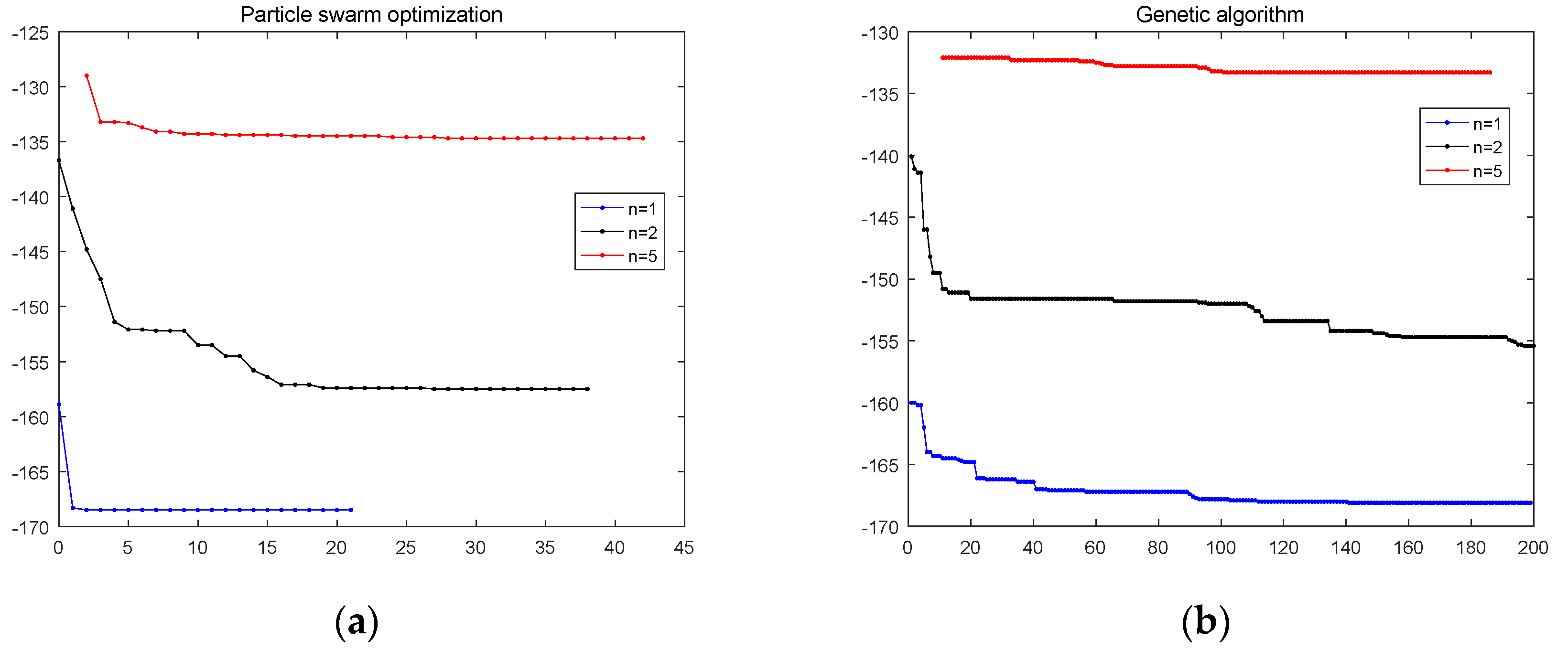
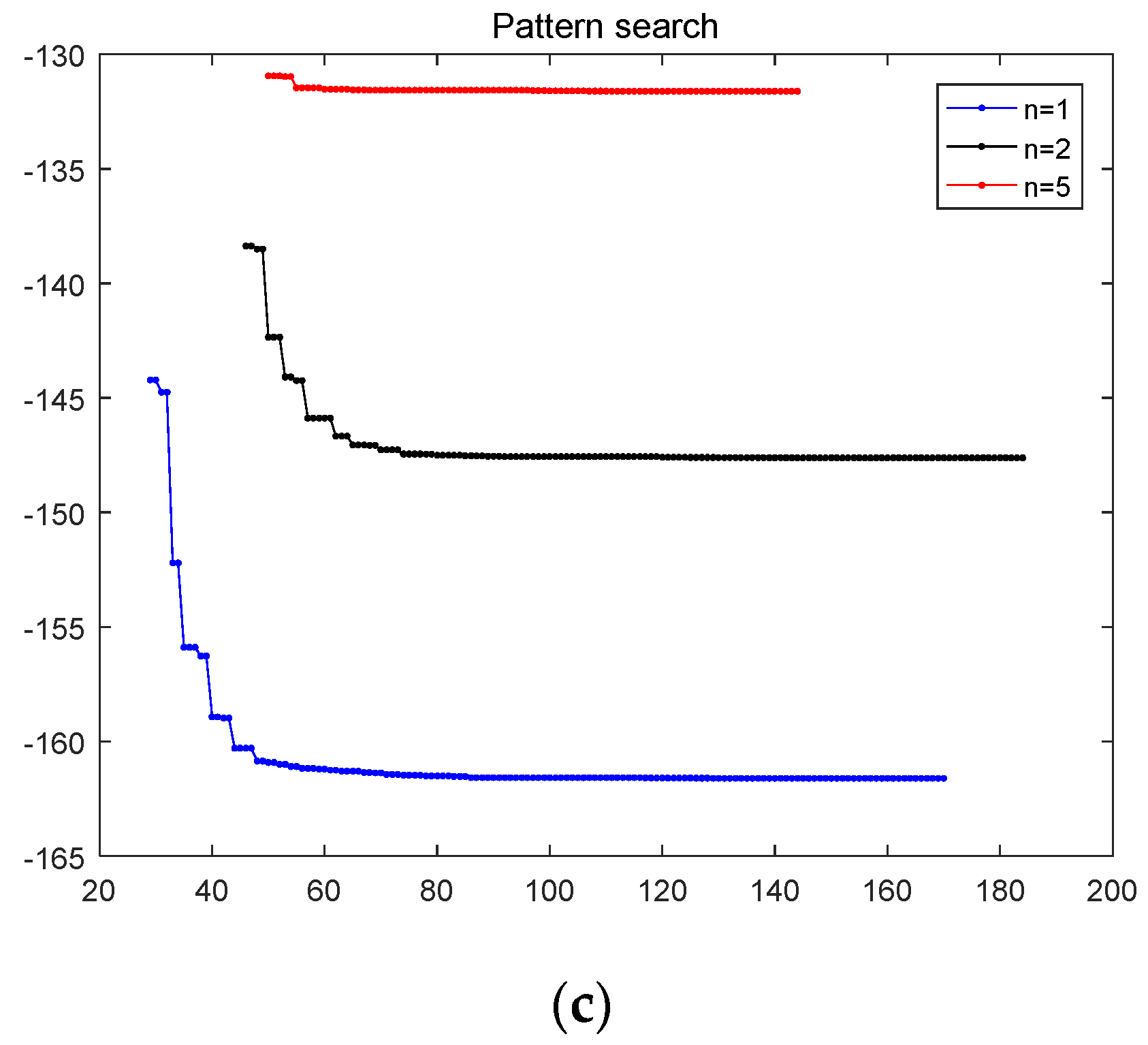
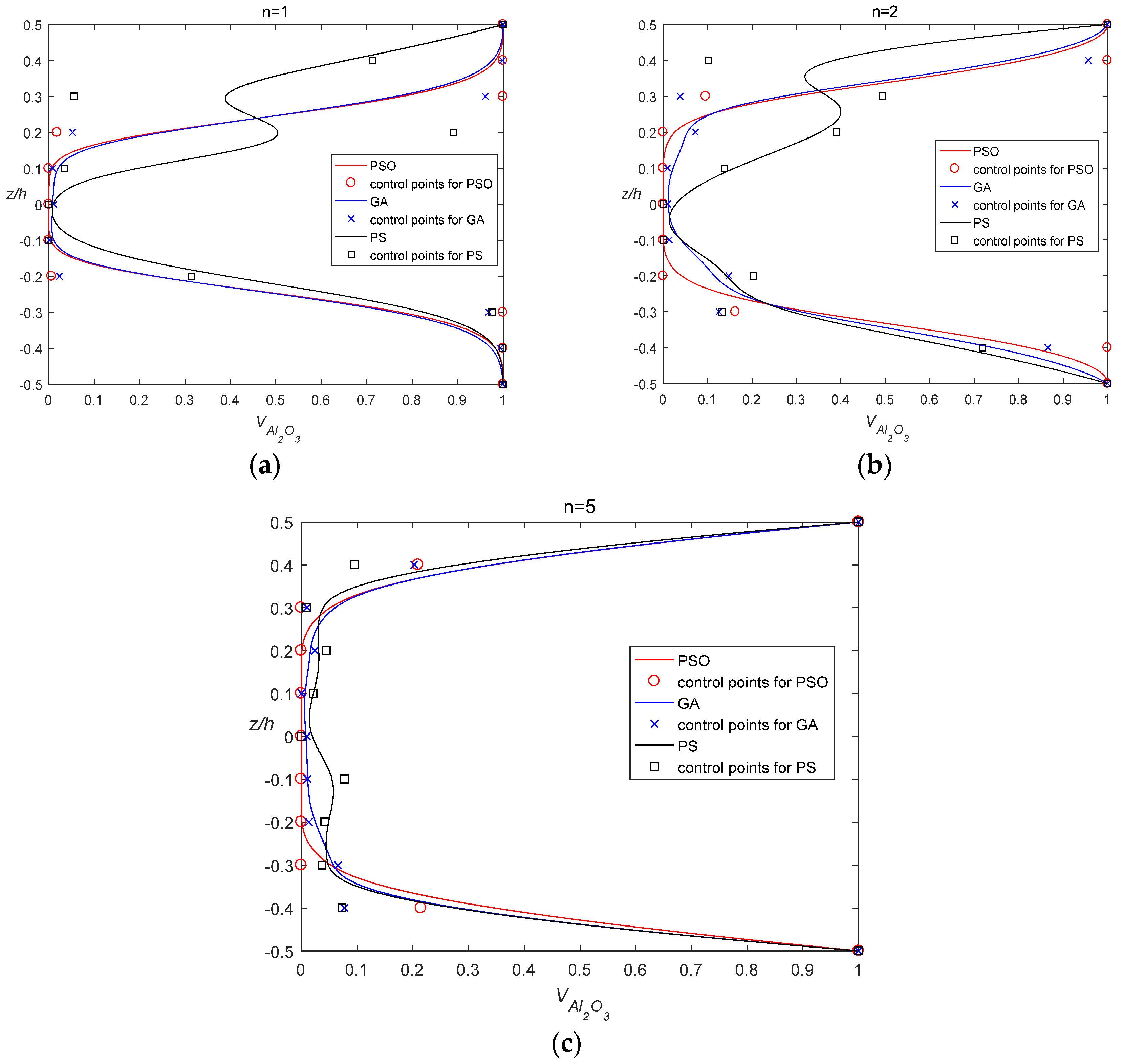
• Since the PS get stuck in the local optimum and cannot obtain the best solution, and the PSO and GA have the same population size, it is concluded that the PSO moves fast towards the optimal solutions, and performs best in comparison with the GA and PS;
• An appropriate distribution of the material constituents can effectively improve the dynamic performance of FG plates. In this study, the performance of the optimal FG plate is presented in comparison with the power-law FG plate, and a great improvement can be observed. Nevertheless, the much thinner graded region may make the FG plate more difficult to fabricate. In this case, the thickness constraint, such as $h/40$ in Equation (48) and $h/60$ in Equation (50), can be adapted to meet the level of the manufacturability while maximizing the mechanical performance of the FG plate.
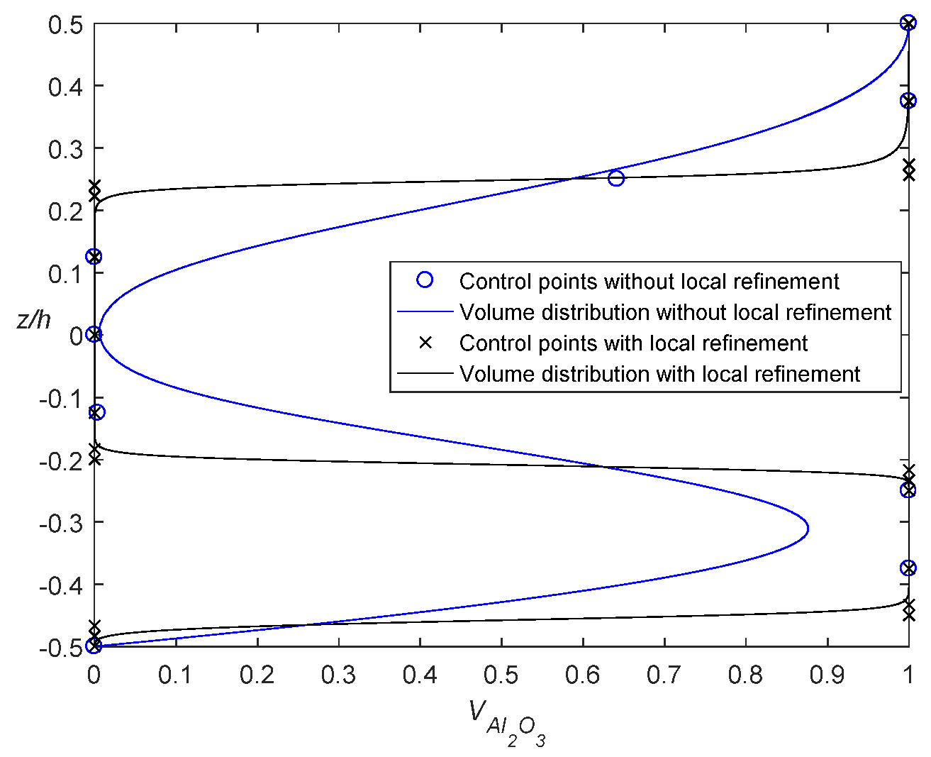
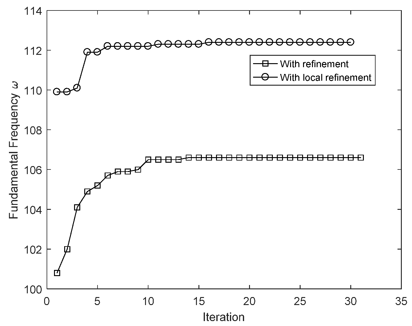
• The local refinement strategy with two parameters is found to be very effective in determining the location and width of graded zones and searching for local optimal solutions. The optimal plates with the local refinement perform better than plates without the local refinement;
• The optimal volume fraction of the FG plate represents a sandwich or laminate plate with graded and homogeneous zones. The presented method can obtain the layers of an optimal laminate plate and locate the FG transition zone.

References

1. Birman, V.; Byrd, L.W. Modeling and Analysis of Functionally Graded Materials and Structures. Appl. Mech. Rev. 2007, 60, 195–216. [Google Scholar] [CrossRef]
2. Wei, X.; Chen, W.; Chen, B.; Sun, L. Singular boundary method for heat conduction problems with certain spatially varying conductivity. Comput. Math. Appl. 2015, 69, 206–222. [Google Scholar] [CrossRef]
3. Keleshteri, M.M.; Asadi, H.; Wang, Q. On the snap-through instability of post-buckled FG-CNTRC rectangular plates with integrated piezoelectric layers. Comput. Methods Appl. Mech. Eng. 2018, 331, 53–71. [Google Scholar] [CrossRef]
4. Keleshteri, M.M.; Asadi, H.; Aghdam, M.M. Nonlinear bending analysis of FG-CNTRC annular plates with variable thickness on elastic foundation. Thin-Walled Struct. 2019, 135, 453–462. [Google Scholar] [CrossRef]
5. Keleshteri, M.M.; Asadi, H.; Wang, Q. Postbuckling analysis of smart FG-CNTRC annular sector plates with surface-bonded piezoelectric layers using generalized differential quadrature method. Comput. Methods Appl. Mech. Eng. 2017, 325, 689–710. [Google Scholar] [CrossRef]
6. Keleshteri, M.M.; Asadi, H.; Wang, Q. Large amplitude vibration of FG-CNT reinforced composite annular plates with integrated piezoelectric layers on elastic foundation. Thin-Walled Struct. 2017, 120, 203–214. [Google Scholar] [CrossRef]
7. Keleshteri, M.M.; Jelovica, J. Nonlinear vibration analysis of bidirectional porous beams. Eng. Comput. 2021, 1–17. [Google Scholar] [CrossRef]
8. Keleshteri, M.M.; Jelovica, J. Beam theory reformulation to implement various boundary conditions for generalized differential quadrature method. Eng. Struct. 2022, 252, 113666. [Google Scholar] [CrossRef]
9. Mohammadzadeh-Keleshteri, M.; Asadi, H.; Aghdam, M.M. Geometrical nonlinear free vibration responses of FG-CNT reinforced composite annular sector plates integrated with piezoelectric layers. Compos. Struct. 2017, 171, 100–112. [Google Scholar] [CrossRef]
10. Mohammadzadeh-Keleshteri, M.; Samie-Anarestani, S.; Assadi, A. Large deformation analysis of single-crystalline nanoplates with cubic anisotropy. Acta Mech. 2017, 228, 3345–3368. [Google Scholar] [CrossRef]
11. Hughes, T.J.R.; Cottrell, J.A.; Bazilevs, Y. Isogeometric analysis: CAD, finite elements, NURBS, exact geometry and mesh refinement. Comput. Methods Appl. Mech. Eng. 2005, 194, 4135–4195. [Google Scholar] [CrossRef] [Green Version]
12. Evans, J.A.; Hiemstra, R.R.; Hughes, T.J.R.; Reali, A. Explicit higher-order accurate isogeometric collocation methods for structural dynamics. Comput. Methods Appl. Mech. Eng. 2018, 338, 208–240. [Google Scholar] [CrossRef]
13. Kumar, V.; Singh, S.J.; Saran, V.H.; Harsha, S.P. Vibration characteristics of porous FGM plate with variable thickness resting on Pasternak’s foundation. Eur. J. Mech.-A Solids 2021, 85, 104124. [Google Scholar] [CrossRef]
14. Van Do, V.N.; Lee, C.-H. Free vibration and transient analysis of advanced composite plates using a new higher-order shear and normal deformation theory. Arch. Appl. Mech. 2021, 91, 1793–1818. [Google Scholar] [CrossRef]
15. Zhong, S.; Zhang, J.; Jin, G.; Ye, T.; Song, X. Thermal bending and vibration of FGM plates with various cutouts and complex shapes using isogeometric method. Compos. Struct. 2021, 260, 113518. [Google Scholar] [CrossRef]
16. Wu, Y.H.; Dong, C.Y.; Yang, H.S.; Sun, F.L. Isogeometric symmetric FE-BE coupling method for acoustic-structural interaction. Appl. Math. Comput. 2021, 393, 125758. [Google Scholar] [CrossRef]
17. Xue, Y.; Jin, G.; Ye, T.; Shi, K.; Zhong, S.; Yang, C. Isogeometric analysis for geometric modelling and acoustic attenuation performances of reactive mufflers. Comput. Math. Appl. 2020, 79, 3447–3461. [Google Scholar] [CrossRef]
18. Taheri, A.H.; Hassani, B. Simultaneous isogeometrical shape and material design of functionally graded structures for optimal eigenfrequencies. Comput. Methods Appl. Mech. Eng. 2014, 277, 46–80. [Google Scholar] [CrossRef]
19. Taheri, A.H.; Hassani, B.; Moghaddam, N.Z. Thermo-elastic optimization of material distribution of functionally graded structures by an isogeometrical approach. Int. J. Solids Struct. 2014, 51, 416–429. [Google Scholar] [CrossRef] [Green Version]
20. Taheri, A.H.; Suresh, K. An isogeometric approach to topology optimization of multi-material and functionally graded structures. Int. J. Numer. Methods Eng. 2017, 109, 668–696. [Google Scholar] [CrossRef]
21. Le-Manh, T.; Lee, J. Stacking sequence optimization for maximum strengths of laminated composite plates using genetic algorithm and isogeometric analysis. Compos. Struct. 2014, 116, 357–363. [Google Scholar] [CrossRef]
22. Ghasemi, H.; Kerfriden, P.; Bordas, S.P.A.; Muthu, J.; Zi, G.; Rabczuk, T. Interfacial shear stress optimization in sandwich beams with polymeric core using non-uniform distribution of reinforcing ingredients. Compos. Struct. 2015, 120, 221–230. [Google Scholar] [CrossRef] [Green Version]
23. Lieu, Q.X.; Lee, J. Modeling and optimization of functionally graded plates under thermo-mechanical load using isogeometric analysis and adaptive hybrid evolutionary firefly algorithm. Compos. Struct. 2017, 179, 89–106. [Google Scholar] [CrossRef]
24. Hao, P.; Feng, S.; Zhang, K.; Li, Z.; Wang, B.; Li, G. Adaptive gradient-enhanced kriging model for variable-stiffness composite panels using Isogeometric analysis. Struct. Multidiscip. Optim. 2018, 58, 1–16. [Google Scholar] [CrossRef]
25. Hao, P.; Yuan, X.; Liu, C.; Wang, B.; Liu, H.; Li, G.; Niu, F. An integrated framework of exact modeling, isogeometric analysis and optimization for variable-stiffness composite panels. Comput. Methods Appl. Mech. Eng. 2018, 339, 205–238. [Google Scholar] [CrossRef]
26. Borden, M.J.; Scott, M.A.; Evans, J.A.; Hughes, T.J.R. Isogeometric finite element data structures based on Bézier extraction of NURBS. Int. J. Numer. Methods Eng. 2011, 87, 15–47. [Google Scholar] [CrossRef]
27. Hedia, H.S.; Mahmoud, N.-A. Design optimization of functionally graded dental implant. Bio-Med. Mater. Eng. 2004, 14, 133–143. [Google Scholar]
28. Tahouneh, V.; Naei, M.H. A novel 2-D six-parameter power-law distribution for three-dimensional dynamic analysis of thick multi-directional functionally graded rectangular plates resting on a two-parameter elastic foundation. Meccanica 2014, 49, 91–109. [Google Scholar] [CrossRef]
29. Qian, L.F.; Batra, R.C. Design of bidirectional functionally graded plate for optimal natural frequencies. J. Sound Vib. 2005, 280, 415–424. [Google Scholar] [CrossRef]
30. Correia, V.M.F.; Madeira, J.F.A.; Araújo, A.L.; Soares, C.M.M. Multiobjective optimization of functionally graded material plates with thermo-mechanical loading. Compos. Struct. 2019, 207, 845–857. [Google Scholar] [CrossRef]
31. Cho, J.R.; Choi, J.H. A yield-criteria tailoring of the volume fraction in metal-ceramic functionally graded material. Eur. J. Mech.-A Solids 2004, 23, 271–281. [Google Scholar] [CrossRef]
32. Ashjari, M.; Khoshravan, M.R. Mass optimization of functionally graded plate for mechanical loading in the presence of deflection and stress constraints. Compos. Struct. 2014, 110, 118–132. [Google Scholar] [CrossRef]
33. Goupee, A.J.; Vel, S.S. Multi-objective optimization of functionally graded materials with temperature-dependent material properties. Mater. Des. 2007, 28, 1861–1879. [Google Scholar] [CrossRef]
34. Do, D.T.T.; Lee, D.; Lee, J. Material optimization of functionally graded plates using deep neural network and modified symbiotic organisms search for eigenvalue problems. Compos. Part B Eng. 2019, 159, 300–326. [Google Scholar] [CrossRef]
35. Scott, M.A.; Borden, M.J.; Verhoosel, C.V.; Sederberg, T.W.; Hughes, T.J.R. Isogeometric finite element data structures based on Bézier extraction of T-splines. Int. J. Numer. Methods Eng. 2011, 88, 126–156. [Google Scholar] [CrossRef]
36. Nguyen, T.-K.; Sab, K.; Bonnet, G. First-order shear deformation plate models for functionally graded materials. Compos. Struct. 2008, 83, 25–36. [Google Scholar] [CrossRef] [Green Version]
37. Bakhtiari-Nejad, F.; Shamshirsaz, M.; Mohammadzadeh, M.; Samie, S. Free Vibration Analysis of FG Skew Plates Based on Second Order Shear Deformation Theory. In Proceedings of the ASME 2014 International Design Engineering Technical Conferences and Computers and Information in Engineering Conference, New York, NY, USA, 17–20 August 2014. [Google Scholar]
38. Reddy, J.N. Analysis of functionally graded plates. Int. J. Numer. Methods Eng. 2000, 47, 663–684. [Google Scholar] [CrossRef]
39. Neves, A.M.A.; Ferreira, A.J.M.; Carrera, E.; Roque, C.M.C.; Cinefra, M.; Jorge, R.M.N.; Soares, C.M.M. A quasi-3D sinusoidal shear deformation theory for the static and free vibration analysis of functionally graded plates. Compos. Part B Eng. 2012, 43, 711–725. [Google Scholar] [CrossRef]
40. Yin, S.; Hale, J.S.; Yu, T.; Bui, T.Q.; Bordas, S.P.A. Isogeometric locking-free plate element: A simple first order shear deformation theory for functionally graded plates. Compos. Struct. 2014, 118, 121–138. [Google Scholar] [CrossRef] [Green Version]
41. Piegl, L.A.; Tiller, W. The NURBS Book, 2nd ed.; Springer: New York, NY, USA, 1997. [Google Scholar]
42. Poli, R.; Kennedy, J.; Blackwell, T. Particle swarm optimization. Swarm Intell. 2007, 1, 33–57. [Google Scholar] [CrossRef]
43. Bennoun, M.; Houari, M.S.A.; Tounsi, A. A novel five-variable refined plate theory for vibration analysis of functionally graded sandwich plates. Mech. Adv. Mater. Struct. 2016, 23, 423–431. [Google Scholar] [CrossRef]
44. Zienkiewicz, O.C.; Xu, Z.; Zeng, L.F.; Samuelsson, A.; Wiberg, N.-E. Linked interpolation for Reissner-Mindlin plate elements: Part I—A simple quadrilateral. Int. J. Numer. Methods Eng. 1993, 36, 3043–3056. [Google Scholar] [CrossRef]
Figure 1. Schematic geometry of an FGM Mindlin plate.
Crystals 12 00830 g001
Figure 2. Example of 100 particles generated by different operators: (a) uniform pseudorandom generator, (b) Latin hypercube, and (c) Latin hypercube improved by maximizing the minimum distance between points.
Crystals 12 00830 g002
Figure 3. A square plate with 18 × 18 control points and 15 × 15 elements by using cubic NURBS basis function: (a) control mesh, (b) physical mesh.
Crystals 12 00830 g003
Figure 4. The history of the objective function for frequency difference maximization with different algorithms:(a) Particle swarm optimization; (b) Genetic algorithm; (c) Pattern search.
Crystals 12 00830 g004aCrystals 12 00830 g004b
Figure 5. Volume fraction distribution for different mass constraints with different index: (a) n = 1; (b) n = 2; (c) n = 5.
Crystals 12 00830 g005
Figure 6. Volume fraction distribution for different boundary conditions: (a) SFSF; (b) SSSS; (c) SCSC; (d) CCCC.
Crystals 12 00830 g006
Figure 7. The history of the objective function for fundamental frequency of the FG plate with mass constraint.
Crystals 12 00830 g007
Figure 8. Volume fraction distribution with local refinement.
Crystals 12 00830 g008
Figure 9. The history of the objective function of the local refinement.
Crystals 12 00830 g009
Figure 10. Volume fraction distribution for optimization with and without local refinement.
Crystals 12 00830 g010
Figure 11. The iteration history of the objective function for frequency optimization with and without refinement.
Crystals 12 00830 g011