A Novel Photo Elasto-Thermodiffusion Waves with Electron-Holes in Semiconductor Materials with Hyperbolic Two Temperature

Abstract

In this paper, a novel mathematical—physical model of the generalized elasto-thermodiffusion (hole/electron interaction) waves in semiconductor materials is studied when the hyperbolic two-temperature theory in the two-dimensional (2D) deformation is taken into account. Shear (purely transverse) waves are dissociated from the remainder of the motion and remain unaffected by external fields. The coupled system of partial differential equations of the main interacting fields has been solved. Using the Laplace transform method, the governing equations of motion and heat conduction can be formulated in 2D. The hole charge carrier, displacement, thermal, and plasma boundary conditions are applied on the interface adjacent to the vacuum to obtain the basic physical quantities in the Laplace domain. The inversion of the Laplace transform with the numerical method is applied to obtain the complete solutions in the time domain for the main physical fields under investigation. The effects of thermoelastic, the phase-lag of the temperature gradient and the phase-lag of the heat flux, the hyperbolic two-temperature parameter, and comparing between silicon and germanium materials on the displacement component, carrier density, hole charge carrier, and temperature distribution have been discussed and obtained graphically.

1. Introduction

Semiconductors are electrically insulating materials under normal conditions; for example, glass. However, when materials are exposed to laser beams and light or sunlight, they cause an internal excitation of electrons, which leads to their spread on the surface to become electrically conductive materials; for example, copper. That is, semiconductors deform their physical properties when exposed to external variables such as a gradual increase in temperature. From this standpoint, semiconductors are important in all modern industries such as the manufacture of electronics, solar cells, and sensors. Where semiconductors are exposed to direct radiation, electrons move towards the surface, leaving gaps behind in a process called electronic deformation (ED). As a direct result of the movement of excited electrons towards the surface, an elastic thermal deformation (ETD) occurs. Therefore, when studying semiconductors, the theory of photo-thermoelasticity should be used to examine the governing equations of the system.

Lord Rayleigh [1] predicted the existence of Rayleigh waves concerning the earthquake spectrum analysis. Rayleigh waves travel at about 10 times the speed of sound in the air along the earth’s surface. Surface waves are well understood to be acoustic or elastic and they can also be coupled with other physical fields such as piezoelectric, magnetic, electric, diffusion, and so on. In the context of coupled thermoelasticity, Lockett and colleagues [2] investigated the propagation of thermoelastic Rayleigh waves. Chandrasekharaiah [3] modified the Fourier law of heat conduction and constitutive relations to obtain a hyperbolic equation for heat conduction. These models account for the time required to accelerate heat flow and temperature-strain field coupling.

Maruszewski [4] investigated the interaction of elastic, thermal, and diffusion fields of charge carriers in semiconductors after mathematically formulating the problem. Maruszewski [4] also investigated the propagation of thermodiffusion surface waves in semiconductor materials using his phenomenological model, which includes relaxation times of heat and charge carriers as well as carrier lifetimes. He also presented numerical solutions to his model’s problems in these situations. However, his investigations were eventually limited to some special and specific situations; they remained departed from the general solution of the said model, ignoring the presence of some of the interacting fields included in the basic governing equations at the same time. Sharma and Thakur [5] investigated the propagation of plane harmonic elasto-thermodiffusive (ETNP) waves in semiconductor materials by simplifying the Maruszewski model of governing equations by introducing non-dimensional quantities. In an infinite semiconductor, four coupled longitudinal waves, namely the quasi-thermoelastic (QTE), quasi-elastodiffusive (QEN/QEP), quasi-thermodiffusive (QTN/QTP), and quasi-thermal (T-mode), as well as decoupled shear waves, are discovered to exit. Sharma et al. [6] studied the propagation of elasto-thermodiffusive (ETN) surface waves in a semiconductor material half-space. Lotfy et al. [7] proposed an elastic-thermodiffusion (ETD) model for the semiconductor material that is coupled between holes and electrons. This model is described by photothermal excitation in generalized thermoelasticity theory. Aldwoah et al. [8] investigated the coupling of electrons and holes in a theoretical mathematical—physical model of a semiconductor medium. During photothermal transport processes, the elasto-thermodiffusion (ETD) theory is taken into account. Hobiny and Abbas [9] studied an elastic semiconductor medium according to the generalized thermo-diffusion theory, when the physical constant of the medium depends on the change in temperature. On the other hand, Abouelregal et al. [10] investigated the impact of an excess carrier on semiconductor material in the context of the Green and Naghdi theory. Awwad et al. [11] took into consideration the functionally graded influence on the excited semiconductor medium by laser pulses.

According to the formulations of the deformable body theory, the conductive temperature and the thermodynamic temperature are two distinct temperatures that affect how much heat may be transferred [12,13]. The difference between the two temperatures, which coincide when the heat source is absent, is discussed by Chen et al. [14]. The existence of two-temperature thermoelasticity theory, structural stability, convergence, and spatial behavior of elastic media was demonstrated by Quintanilla and Tien [15]. A novel model of the two-temperature theory for generalized thermoelasticity was developed by Youssef [16,17], yet this theory contains a paradox. The paradox relates to the infinitely fast thermal wave propagation that is predicted by this theory. The contradiction was resolved by Youssef and El-Bary [18] when they devised two types of separate temperatures that are dependent on the acceleration of thermal and conductive temperature. Lotfy et al. [19] studied a novel model which describes the photothermal excitation under the impact of the theory of magneto-hyperbolic two-temperature during thermo-diffusion processes of the semiconducting medium. On the other hand, Lotfy et al. [20] studied the semiconductor medium when the piezo-photo-thermoelasticity theory during the hyperbolic two-temperature theory is taken into account.

The generalized elasto-thermo-diffusion (ETD) waves in semiconductor materials for two-dimensional (2D) deformation are discussed and studied when the electrons/holes interaction is taken into account. The governing equations of motion and heat conduction are solved using the Laplace transform method with the hyperbolic two-temperature theory. To obtain the main physical quantities in the Laplace domain, the hole charge carrier, displacement, thermal, and plasma boundary conditions are applied as boundary conditions to the interface adjacent to the vacuum. The inverting process is then carried out numerically using an efficient programming language. Finally, normal displacement, carrier density, hole charge carrier, and temperature distribution were computed numerically and graphically represented.

2. Basic Equations

The unbounded, homogeneous, isotropic, thermoelastic semiconductor at a uniform temperature $T_0$ in an undisturbed state is taken into consideration. The following quantities $u(x,z,t)$, $T(x,z,t)$, $N(x,z,t),$ $H(x,z,t)$ and $\varphi (x,z,t),$ are the displacement vector, temperature (thermodynamic) change of the medium at any time $t$, carrier density (intensity), the hole charge carrier, and the conductive temperature, respectively. The basic governing equations of motion, plasma, holes, and heat conduction according to the hyperbolic two-temperature theory in the absence of body forces and heat sources for such materials in 2D are [8]:

$$\left.\begin{array}{l}K(1+{\tau }_{\theta }\frac{\partial }{\partial t})\left(\frac{{\partial }^2\phi }{\partial x^2}+\frac{{\partial }^2\phi }{\partial z^2}\right)+m_{nq}\left(\frac{{\partial }^{2}N}{\partial x^2}+\frac{{\partial }^{2}N}{\partial z^2}\right)+m_{hq}\left(\frac{{\partial }^{2}H}{\partial x^2}+\frac{{\partial }^{2}H}{\partial z^2}\right)-\\ (1+{\tau }_q\frac{\partial }{\partial t})\left[\rho \hspace{0.17em}{C}_e\frac{\partial T}{\partial t}+\rho \hspace{0.17em}{T}_0{\alpha }_n\frac{\partial N}{\partial t}+\rho \hspace{0.17em}{T}_0{\alpha }_h\frac{\partial H}{\partial t}+\hspace{0.17em}{T}_0\gamma \frac{\partial }{\partial t}\left(\frac{\partial u}{\partial x}+\frac{\partial w}{\partial z}\right)\right]-\hspace{0.17em}\\ \rho (a_1^n\frac{\partial N}{\partial t}+a_1^h\frac{\partial H}{\partial t})\hspace{0.17em}=\left[\frac{\rho a_1^n}{t^n}N+\frac{\rho a_1^h}{t^h}H\right]\end{array}\right\},$$

(1)

$$\left.\begin{array}{l}{m}_{qn}\left(\frac{{\partial }^{2}T}{\partial x^2}+\frac{{\partial }^{2}T}{\partial z^2}\right)+D_n\rho \left(\frac{{\partial }^{2}N}{\partial x^2}+\frac{{\partial }^{2}N}{\partial z^2}\right)-\rho (1-a_2^n\hspace{0.17em}{T}_0{\alpha }_n+t^n\frac{\partial }{\partial t})\frac{\partial N}{\partial t}\\ \hspace{1em}\hspace{1em}\hspace{1em}-a_2^n\left[\rho \hspace{0.17em}{C}_e\frac{\partial T}{\partial t}+\rho \hspace{0.17em}{T}_0{\alpha }_h\frac{\partial H}{\partial t}+\hspace{0.17em}{T}_0\gamma \frac{\partial }{\partial t}\left(\frac{\partial u}{\partial x}+\frac{\partial w}{\partial z}\right)\right]\hspace{0.17em}\hspace{0.17em}=-\frac{\rho }{t_1^n}(1+t^n\frac{\partial }{\partial t})N\end{array}\right\},$$

(2)

$$\left.\begin{array}{l}{m}_{qh}\left(\frac{{\partial }^{2}T}{\partial x^2}+\frac{{\partial }^{2}T}{\partial z^2}\right)+D_h\rho \left(\frac{{\partial }^{2}H}{\partial x^2}+\frac{{\partial }^{2}H}{\partial z^2}\right)-\rho (1-a_2^h\hspace{0.17em}{T}_0{\alpha }_h+t^h\frac{\partial }{\partial t})\frac{\partial H}{\partial t}\\ \hspace{1em}\hspace{1em}\hspace{1em}-a_2^h\left[\rho \hspace{0.17em}{C}_e\frac{\partial T}{\partial t}+\rho \hspace{0.17em}{T}_0{\alpha }_n\frac{\partial N}{\partial t}+\hspace{0.17em}{T}_0\gamma \frac{\partial }{\partial t}\left(\frac{\partial u}{\partial x}+\frac{\partial w}{\partial z}\right)\right]\hspace{0.17em}\hspace{0.17em}=-\frac{\rho }{t_1^h}(1+t^h\frac{\partial }{\partial t})H\end{array}\right\},$$

(3)

$$\rho \hspace{0.17em}\frac{{\partial }^{2}u}{\partial t^2}=(2\mu +\lambda \hspace{0.33em})\frac{{\partial }^{2}u}{\partial x^2}+\mu \frac{{\partial }^{2}u}{\partial z^2}-\gamma (1+{\tau }_{\theta }\frac{\partial }{\partial t})\frac{\partial T}{\partial x}\hspace{0.17em}-{\delta }_n\frac{\partial N}{\partial x}-{\delta }_h\frac{\partial H}{\partial x},$$

(4)

$$\rho \hspace{0.17em}\frac{{\partial }^{2}w}{\partial t^2}=(2\mu +\lambda \hspace{0.33em})\frac{{\partial }^{2}w}{\partial z^2}+\mu \frac{{\partial }^{2}w}{\partial x^2}-\gamma (1+{\tau }_{\theta }\frac{\partial }{\partial t})\frac{\partial T}{\partial z}\hspace{0.17em}-{\delta }_n\frac{\partial N}{\partial z}-{\delta }_h\frac{\partial H}{\partial z}.$$

(5)

The relation between the conduction of heat and thermodynamic heat according to the hyperbolic two-temperature theory takes the form [17]:

$$\hspace{0.17em}\ddot{\varphi }-\ddot{T}=\beta \hspace{0.17em}{\nabla }^2\varphi .$$

(6)

where $\beta$ is a positive constant, it is called the hyperbolic two-temperature parameter. The constitutive equation in 2D takes the following form [21]:

$${\sigma }_{xx}=(2\mu +\lambda )\frac{\partial u}{\partial x}+\lambda \frac{\partial w}{\partial z}-(\gamma (1+{\tau }_{\theta }\frac{\partial }{\partial t})T+{\delta }_{n}N)-{\delta }_{h}H,$$

(7)

$${\sigma }_{zz}=(2\mu +\lambda )\frac{\partial w}{\partial z}+\lambda \frac{\partial u}{\partial x}-(\gamma (1+{\tau }_{\theta }\frac{\partial }{\partial t})T+{\delta }_{n}N)-{\delta }_{h}H,$$

(8)

$${\sigma }_{xz}=\mu (\frac{\partial u}{\partial z}+\frac{\partial w}{\partial x})-{\delta }_{h}H.$$

(9)

where $\mu ,\lambda$ is Lame’s elastic constants, $\rho$ is the density of the semiconductor, ${\delta }_h$ and ${\delta }_n$ are the elasto-diffusive constants of electrons and holes, ${\alpha }_t$ is the linear thermal expansion coefficient, $C_e$ is the solid plate specific heat co-efficient at constant strain, and $d_n$ is the difference between conductive deformation potential and valence band. $k$ is the thermal conductivity and $T_0$ is the rest temperature. The quantities $m_{nq},m_{qn},m_{hq},m_{qh}$ are the Peltier-Dufour-Seebeck-Soret-like constants. $D_n,D_h$ are the diffusion coefficients of electrons and holes. The quantities $t^n$ and $t^h$ are the relaxation times of heat and electron. ${\alpha }_h$ and ${\alpha }_n$ are thermo-diffusive constants of holes and electrons, respectively. $t_{\theta }$ and $t_q$ are the two thermal memories. On the other hand, the quantities $a_{Qn},a_{Qh},a_Q,a_n,\hspace{0.17em}{a}_h$ represent the flux-like constants. The other notations can be rewritten as: $\gamma =(3\lambda +2\mu ){\alpha }_t$, $a_1^n=\frac{a_{Qn}}{a_Q}$, $a_1^h=\frac{a_{Qh}}{a_Q}$, $a_2^n=\frac{a_{Qn}}{a_n}$ and $a_2^h=\frac{a_{Qh}}{a_h}$.

In the non-dimensional form, two scalar potential functions can be inserted, which take the form: $u=\frac{\partial \mathrm{\Pi }}{\partial x}+\frac{\partial \mathsf{\Psi }}{\partial z}$ and $w=\frac{\partial \mathrm{\Pi }}{\partial z}-\frac{\partial \mathsf{\Psi }}{\partial x}$.

For simplicity, the following non-dimensional variables are used:

$$\begin{array}{l}(x^{\prime },z^{\prime },u^{\prime },w^{\prime })=\frac{{\omega }^{*}(x,z,u,w)}{C_T}, (t^{\prime },{{\tau }^{\prime }}_q,{{\tau }^{\prime }}_{\theta },t^{n^{\prime }},t^{h^{\prime }},t_1^{n^{\prime }},t_1^{h^{\prime }})={\omega }^{*}(t,\hspace{0.33em}{\tau }_q,{\tau }_{\theta },t^n,t^h,t_1^n,t_1^h), T^{\prime }=\frac{T}{T_0},c^2=\frac{C_T^2}{C_L^2,}\\ {{\sigma }^{\prime }}_{ij}=\frac{{\sigma }_{ij}}{\mu }, N^{\prime }=\frac{N}{n_0}, H^{\prime }=\frac{H}{h_0}, C_T^2=\frac{2\mu +\lambda }{\rho }, C_L^2=\frac{\mu }{\rho }, {\omega }^{*}=\frac{C_e(\lambda +2\mu )}{K}, {\overline{\lambda }}_n=\frac{{\delta }_n{n}_0}{\gamma T_0}, {\overline{\lambda }}_h=\frac{{\delta }_h{h}_0}{\gamma T_0}\\ ,(x^{\prime },z^{\prime },\hspace{0.33em}{u}^{\prime },w^{\prime })=\frac{(x,z,\hspace{0.33em}u,w)}{C_T{t}^{*}},\hspace{1em}\hspace{1em}(t^{\prime },{{\tau }^{\prime }}_q,{{\tau }^{\prime }}_{\theta })=\frac{(t,\hspace{0.33em}{\tau }_q,{\tau }_{\theta })}{t^{*}},\hspace{1em}\hspace{1em}(T^{\prime },\hspace{0.33em}{\varphi }^{\prime })=\frac{\gamma (T,\varphi )}{2\mu +\lambda },\hspace{1em}\hspace{1em}{{\sigma }^{\prime }}_{ij}=\frac{{\sigma }_{ij}}{\mu },\\ N^{\prime }=\frac{{\delta }_{n}N}{2\mu +\lambda },\hspace{1em}\hspace{1em}\hspace{1em}({\mathrm{\Pi }}^{\prime },{\psi }^{\prime })=\frac{(\mathrm{\Pi },\psi )}{{(C_T{t}^{*})}^2},\hspace{1em}\hspace{1em}\hspace{1em}{Q}^{\prime }=\frac{\gamma \hspace{0.17em}{t}^{*}{}^2}{\rho k}Q,\hspace{1em}\hspace{1em}\hspace{1em}{g}^{\prime }=\frac{t^{*}}{C_T}g.\end{array}$$

(10)

The dashes are dropped for convenience in Equations (1)–(9) by using Equation (10), yield:

$$\left.\begin{array}{l}(1+{\tau }_{\theta }\frac{\partial }{\partial t}){\nabla }^2\varphi -(1+{\tau }_q\frac{\partial }{\partial t})\frac{\partial }{\partial t}T+\left\{{\beta }_1{\nabla }^2-{\beta }_2(1+{\tau }_q\frac{\partial }{\partial t})\frac{\partial }{\partial t}-{\beta }_3\frac{\partial }{\partial t}-{\beta }_4\right\}N+\\ \left\{{\beta }_5{\nabla }^2-(1+{\tau }_q\frac{\partial }{\partial t}){\beta }_6\frac{\partial }{\partial t}-{\beta }_7\right\}H-(1+{\tau }_q\frac{\partial }{\partial t}){\epsilon }_1\frac{\partial }{\partial t}{\nabla }^2\mathrm{\Pi }=0\end{array}\right\},$$

(11)

$$\left.\begin{array}{l}\left\{{\nabla }^2-{\beta }_8\frac{\partial }{\partial t}\right\}T+\left\{{\beta }_9{\nabla }^2-({\beta }_{10}+t^n\frac{\partial }{\partial t}){\beta }_{11}+(1+t^n\frac{\partial }{\partial t})\frac{{\beta }_{11}}{t_1^n}\right\}N\hspace{0.17em}\\ -{\beta }_{12}\frac{\partial H}{\partial t}-{\beta }_{13}\hspace{0.17em}\frac{\partial }{\partial t}{\nabla }^2\mathrm{\Pi }\hspace{0.17em}=0\end{array}\right\},$$

(12)

$$\left.\begin{array}{l}\left\{{\nabla }^2-{\beta }_{14}\frac{\partial }{\partial t}\right\}T+\left\{{\beta }_{15}{\nabla }^2-{\beta }_{16}({\beta }_{17}+t^h\frac{\partial }{\partial t})\frac{\partial }{\partial t}+(1+t^h\frac{\partial }{\partial t})\frac{{\beta }_{16}}{t_1^h}\right\}H\\ -{\beta }_{18}\frac{\partial N}{\partial t}-{\beta }_{19}\frac{\partial }{\partial t}{\nabla }^2\mathrm{\Pi }=0\end{array}\right\},$$

(13)

$$\left\{{\nabla }^2-\frac{{\partial }^2}{\partial t^2}\right\}\mathrm{\Pi }-(1+{\tau }_{\theta }\frac{\partial }{\partial t})T-N-{\beta }_{20}H=0,$$

(14)

$$\left\{{\nabla }^2-\alpha \frac{{\partial }^2}{\partial t^2}\right\}\mathsf{\Psi }=0,$$

(15)

$$\ddot{\varphi }-{\beta }_{21}{\nabla }^2\varphi =\ddot{T},$$

(16)

$${\mathsf{\sigma }}_{\mathit{xx}}={\beta }_{22}\frac{{\partial }^2\mathrm{\Pi }}{\partial x^2}+{\beta }_{23}\frac{{\partial }^2\mathrm{\Pi }}{\partial z^2}+2\frac{{\partial }^2\mathsf{\Psi }}{\partial z\partial x}-{\beta }_{22}\left((\hspace{0.17em}(1+{\tau }_{\theta }\frac{\partial }{\partial t})T\hspace{0.17em}+N)\right)-{\beta }_{20}H,$$

(17)

$${\mathsf{\sigma }}_{\mathit{zz}}={\beta }_{22}\frac{{\partial }^2\mathrm{\Pi }}{\partial z^2}+{\beta }_{23}\frac{{\partial }^2\mathrm{\Pi }}{\partial x^2}-2\frac{{\partial }^2\mathsf{\Psi }}{\partial z\partial x}-{\beta }_{22}\left((\hspace{0.17em}(1+{\tau }_{\theta }\frac{\partial }{\partial t})T\hspace{0.17em}+N)\right)-{\beta }_{20}H,$$

(18)

$${\mathsf{\sigma }}_{\mathit{xz}}=\frac{{\partial }^2\mathsf{\Psi }}{\partial z^2}+2\frac{{\partial }^2\mathrm{\Pi }}{\partial x\partial z}-\frac{{\partial }^2\mathsf{\Psi }}{\partial x^2}.$$

(19)

where

$$\begin{array}{l}{\beta }_1=\frac{m_{nq}\gamma }{{\delta }_n\hspace{0.17em}K}\hspace{0.17em}\hspace{0.17em}\hspace{0.17em},{\beta }_2=\frac{T_0{\alpha }_n\gamma }{{\delta }_n{C}_e},\hspace{0.17em}{\beta }_3=\frac{a_1^n\gamma }{C_e{\delta }_n},{\beta }_4=\frac{{\beta }_3}{{\tau }^n},{\beta }_5=\frac{\gamma m_{hq}\hspace{0.17em}{h}_0}{(2\mu +\lambda )K},{\beta }_6=\frac{T_0\hspace{0.17em}{\alpha }_h\hspace{0.17em}\gamma \hspace{0.17em}{h}_0{t}^{\ast }}{K},\\ {\beta }_7=\frac{a_1^h\gamma t^{\ast }}{K},{\beta }_8=\frac{a_2^{n}K}{m_{qn}},{\beta }_9=\frac{D_n\rho {\alpha }_t}{m_{qn}\hspace{0.17em}{d}_n},{\beta }_{10}=1-a_2^n{T}_0{\alpha }_n,{\beta }_{11}=\frac{{\alpha }_{t}K}{m_{qn}\hspace{0.17em}{d}_n{C}_e},{\beta }_{12}=\frac{a_2^n\gamma h_0{\alpha }_h{t}^{\ast }}{m_{qn}},\\ {\beta }_{13}=\frac{a_2^n{\gamma }^2{T}_0{t}^{\ast }}{\rho \hspace{0.17em}{m}_{qn}},{\beta }_{14}=a_2^h\frac{K}{m_{qh}},{\beta }_{15}=\frac{D_n{h}_0\gamma }{C_T^2\hspace{0.17em}{m}_{qh}},{\beta }_{16}=\frac{\gamma h_0{t}^{\ast }}{m_{qh}},{\beta }_{17}=1-a_2^h{T}_0{\alpha }_n,{\beta }_{18}=\frac{a_2^h\gamma T_0{\alpha }_{h}K}{m_{qh}{\delta }_n{C}_e},\\ {\beta }_{19}=\frac{a_2^h{\gamma }^2{T}_0\hspace{0.17em}{t}^{\ast }}{m_{qh}\rho },{\beta }_{20}=\frac{{\delta }_h{h}_0}{(2\mu +\lambda )},{\beta }_{21}=\frac{\beta }{C_T{}^2},{\beta }_{22}=\frac{2\mu +\lambda }{\mu },{\beta }_{23}=\frac{\lambda }{\mu },{\epsilon }_1=\frac{T_0{\gamma }^2{t}^{\ast }}{\rho K},\alpha =\frac{K}{\mu C_e}\end{array}$$

The parameter ${\epsilon }_1$ can be called the thermoelastic coupling parameter. To solve the problem analytically, it is possible to consider the following initial conditions with homogeneity properties so that they can be written as:

$$\begin{array}{l}{\left.\mathrm{\Pi }(x,z,t)\right|}_{t=0}=\hspace{1em}{\left.\frac{\partial \mathrm{\Pi }(x,z,t)}{\partial t}\right|}_{t=0}=0,{\left.\mathsf{\Psi }(x,z,t)\right|}_{t=0}=\hspace{1em}{\left.\frac{\partial \mathsf{\Psi }(x,z,t)}{\partial t}\right|}_{t=0}=0 {\left.T(x,z,t)\right|}_{t=0}={\left.\frac{\partial \left.T(x,z,t)\right|}{\partial t}\right|}_{t=0}=0,\\ {\left.{\sigma }_{xx}(x,z,t)\right|}_{t=0}={\left.\frac{\partial \left.{\sigma }_{xx}(x,z,t)\right|}{\partial t}\right|}_{t=0}=0,\hspace{1em}{\left.{\sigma }_{zz}(x,z,t)\right|}_{t=0}={\left.\frac{\partial \left.{\sigma }_{zz}(x,z,t)\right|}{\partial t}\right|}_{t=0}=0,\hspace{0.17em}\\ {\left.{\sigma }_{xz}(x,z,t)\right|}_{t=0}={\left.\frac{\partial \left.{\sigma }_{xz}(x,z,t)\right|}{\partial t}\right|}_{t=0}=0,\hspace{1em}\hspace{1em}\hspace{1em}{\left.H(x,z,t)\right|}_{t=0}={\left.\frac{\partial H(x,z,t)}{\partial t}\right|}_{t=0}=0,\hspace{0.17em}\\ {\left.N(x,z,t)\right|}_{t=0}={\left.\frac{\partial N(x,z,t)}{\partial t}\right|}_{t=0}=0,\hspace{1em}{\left.\varphi (x,z,t)\right|}_{t=0}={\left.\frac{\partial \left.\varphi (x,z,t)\right|}{\partial t}\right|}_{t=0}=0.\end{array}$$

(20)

3. The Solution of the Problem

The Laplace and Fourier transformations can be used to convert the time—space domain to the Laplace and Fourier domain by using the following definition for any function $\left.\chi (x,z,t)\right|$ as [22,23]:

$$L(\chi (x,z,t)\hspace{0.17em})=\tilde{\chi }(x,z,s)\hspace{0.17em}={\displaystyle \underset{0}{\overset{\infty }{\int }}\chi (x,z,t)\exp (-st)}\hspace{0.17em}d\hspace{0.17em}t,$$

(21)

$$F(\tilde{\chi }(x,z,s)\hspace{0.17em})=\overline{\chi }(x,\zeta ,s)\hspace{0.17em}=\frac{1}{\sqrt{2\pi }}{\displaystyle \underset{-\infty }{\overset{\infty }{\int }}\tilde{\chi }(x,z,s)\exp (-i\zeta z)}\hspace{0.17em}d\hspace{0.17em}t.$$

(22)

Using the above definition of Equations (21) and (22) with applied them of all the main Equations (11)–(19), yield:

$$a_1\left(D^2-{\xi }^2\right)\overline{\varphi }-a_2\overline{T}+\left({\beta }_1{D}^2-a_3\right)\overline{N}+\left({\beta }_5{D}^2-a_4\right)\overline{H}-a_5\left(D^2-{\xi }^2\right)\overline{\mathrm{\Pi }}=0,$$

(23)

$$\left(D^2-a_6\right)\overline{T}+\left({\beta }_9{D}^2-a_7\right)\overline{N}\hspace{0.17em}-a_8\overline{H}-a_9\left(D^2-{\xi }^2\right)\overline{\mathrm{\Pi }}\hspace{0.17em}=0,$$

(24)

$$\left(D^2-a_{10}\right)\overline{T}+\left({\beta }_{15}{D}^2-a_{11}\right)\overline{H}-a_{12}\overline{N}-a_{13}\left(D^2-{\xi }^2\right)\overline{\mathrm{\Pi }}=0,$$

(25)

$$\left(D^2-a_{14}\right)\overline{\mathrm{\Pi }}-a_1\overline{T}-\overline{N}-{\beta }_{20}\overline{H}=0,$$

(26)

$$\overline{T}-(1-a_{16}(D^2-{\xi }^2))\overline{\varphi }=0,$$

(27)

$$\left(D^2-a_{15}\right)\overline{\mathsf{\Psi }}=0,$$

(28)

$${\overline{\mathsf{\sigma }}}_{\mathit{xx}}=\left({\beta }_{22}{D}^2-{\beta }_{23}{\zeta }^2\right)\overline{\mathrm{\Pi }}+2i\zeta D\overline{\mathsf{\Psi }}-{\beta }_{22}\left(a_1\overline{T}\hspace{0.17em}+\overline{N})\right)-{\beta }_{20}\overline{H},$$

(29)

$${\overline{\mathsf{\sigma }}}_{\mathit{zz}}=\left({\beta }_{23}{D}^2-{\beta }_{22}{\zeta }^2\right)\overline{\mathrm{\Pi }}-2i\zeta D\overline{\mathsf{\Psi }}-{\beta }_{22}\left(a_1\overline{T}\hspace{0.17em}+\overline{N})\right)-{\beta }_{20}\overline{H}$$

(30)

$${\overline{\mathsf{\sigma }}}_{\mathit{xz}}=2i\zeta D\overline{\mathrm{\Pi }}-\left(D^2+{\zeta }^2\right)\overline{\mathsf{\Psi }}$$

(31)

where $D=\frac{d}{dx}$, $a_1=(1+{\tau }_{\theta }s)$, $a_2=(1+{\tau }_{q}s)\hspace{0.17em}s$, $a_3=\left({\beta }_1{\xi }^2+{\beta }_2{a}_2+{\beta }_{3}s+{\beta }_4\right)$, $a_4=\left({\beta }_5{\xi }^2+{\beta }_6{a}_2+{\beta }_7\right)$, $a_5=a_2{\epsilon }_1$, $a_6={\xi }^2+{\beta }_{8}s$, $a_7={\beta }_9{\xi }^2+({\beta }_{10}+t^{n}s){\beta }_{11}-(1+t^{n}s)\frac{{\beta }_{11}}{t_1^n}$, $a_8={\beta }_{12}s,a_9={\beta }_{13}s$, $a_{10}={\xi }^2+{\beta }_{14}s$, $a_{11}={\beta }_{15}{\xi }^2+({\beta }_{17}+t^{h}s){\beta }_{16}-(1+t^{h}s)\frac{{\beta }_{16}}{t_1^h}$, $a_{12}={\beta }_{18}s,a_{13}={\beta }_{19}s$, $a_{14}={\xi }^2+s^2,a_{15}={\xi }^2+\alpha$, $a_{16}=\frac{{\beta }_{21}}{s^2}$.

Eliminating $\hspace{0.17em}\overline{T},\hspace{0.17em}\overline{N},\overline{\varphi },\overline{\mathrm{\Pi }}$ and $\overline{H}$ between Equations (23)–(27), yields:

$$(D^{10}-{\Delta }_1{D}^8+{\Delta }_2{D}^6-{\Delta }_3{D}^4+{\Delta }_4{D}^2-{\Delta }_5)\left\{\overline{\mathrm{\Pi }},\overline{N},\overline{T},\overline{H},\overline{\varphi }\right\}(x,\zeta ,s)=0.$$

(32)

where

$${\Delta }_1=\frac{-1}{(a_{16}{\beta }_1{\beta }_{15}+a_{16}{\beta }_5{\beta }_9)}\left\{\begin{array}{l}-{\xi }^2{a}_{16}{\beta }_1{\beta }_{15}-{\xi }^2{a}_{16}{\beta }_5{\beta }_9-a_1{a}_5{a}_{16}{\beta }_9{\beta }_{15}-a_1{a}_9{a}_{16}{\beta }_1{\beta }_{15}-a_1{a}_{13}{a}_{16}{\beta }_5{\beta }_9\\ -a_2{a}_{16}{\beta }_9{\beta }_{15}-a_5{a}_{16}{\beta }_9{\beta }_{20}-a_6{a}_{16}{\beta }_1{\beta }_{15}-a_9{a}_{16}{\beta }_1{\beta }_{20}-a_{10}{a}_{16}{\beta }_5{\beta }_9+a_{13}{a}_{16}{\beta }_1{\beta }_{20}\\ -a_{14}{a}_{16}{\beta }_1{\beta }_{15}-a_{14}{a}_{16}{\beta }_5{\beta }_9-a_1{\beta }_9 {\beta }_{15}-a_3{a}_{16}{\beta }_{15}-a_4{a}_{16}{\beta }_9-a_{15}{a}_{16}{\beta }_{15}{a}_7{a}_{16}{\beta }_5-a_8{a}_{16}{\beta }_1\\ +a_9{a}_{16}{\beta }_5-a_{11}{a}_{16}{\beta }_1-a_{12}{a}_{16}{\beta }_5-a_{13}{a}_{16}{\beta }_5-{\beta }_1{\beta }_{15}-{\beta }_5{\beta }_9\end{array}\right\}$$

$${\Delta }_2=\frac{1}{(a_{16}{\beta }_1{\beta }_{15}+a_{16}{\beta }_5{\beta }_9)}\left\{\begin{array}{l}2{\xi }^2{a}_1{a}_5{a}_{16}{\beta }_9{\beta }_{15}+2{\xi }^2{a}_1{a}_9{a}_{16}{\beta }_1{\beta }_{15}+2{\xi }^2{a}_1{a}_{13}{a}_{16}{\beta }_5{\beta }_9+{\xi }^2{a}_2{a}_{16}{\beta }_9{\beta }_{15}+\\ 2{\xi }^2{a}_5{a}_{16}{\beta }_9{\beta }_{20}+{\xi }^2{a}_6{a}_{16}{\beta }_1{\beta }_{15}+2{\xi }^2{a}_9{a}_{16}{\beta }_{1}b[20]+{\xi }^2{a}_{10}{a}_{16}{\beta }_5{\beta }_9-\\ 2{\xi }^2{a}_{13}{a}_{16}{\beta }_1{\beta }_{20}+{\xi }^2{a}_{14}{a}_{16}{\beta }_1{\beta }_{15}+{\xi }^2{a}_{14}{a}_{16}{\beta }_5{\beta }_9+{\xi }^2{a}_1{\beta }_9{\beta }_{15}+{\xi }^2{a}_3{a}_{16}{\beta }_{15}+\\ {\xi }^2{a}_4{a}_{16}{\beta }_9+2{\xi }^2{a}_5{a}_{16}{\beta }_{15}+{\xi }^2{a}_7{a}_{16}{\beta }_5+{\xi }^2{a}_8{a}_{16}{\beta }_1-2{\xi }^2{a}_9{a}_{16}{\beta }_5+{\xi }^2{a}_{11}{a}_{16}{\beta }_1\\ +{\xi }^2{a}_{12}{a}_{16}{\beta }_5+2{\xi }^2{a}_{13}{a}_{16}{\beta }_5+a_1{a}_3{a}_9{a}_{16}{\beta }_{15}+a_1{a}_4{a}_{13}{a}_{16}{\beta }_9+a_1{a}_5{a}_7{a}_{16}{\beta }_{15}+\\ a_1 a_5{a}_{11}{a}_{16}{\beta }_9+a_1{a}_7{a}_{13}{a}_{16}{\beta }_5+a_1{a}_8{a}_{13} a_{16}{\beta }_1+a_1{a}_9{a}_{11}{a}_{16}{\beta }_1+a_1{a}_9{a}_{12}{a}_{16}{\beta }_5-\\ a_2{a}_{13}{a}_{16}{\beta }_9{\beta }_{20}+a_2{a}_{14}{a}_{16}{\beta }_9{\beta }_{15}+a_5{a}_{10}{a}_{16}{\beta }_9{\beta }_{20}-a_6{a}_{13}{a}_{16}{\beta }_1{\beta }_{20}+a_6{a}_{14}{a}_{16}{\beta }_1{\beta }_{15}+\\ a_9{a}_{10}{a}_{16}{\beta }_1{\beta }_{20}+a_{10}{a}_{14}{a}_{16}{\beta }_5{\beta }_9+a_1{a}_5{\beta }_9{\beta }_{15}+a_1{a}_9{\beta }_1{\beta }_{15}+a_1{a}_{13}{\beta }_5{\beta }_9-a_1{a}_{13}{\beta }_9{\beta }_{20}\\ +a_1{a}_{14}{\beta }_9{\beta }_{15}+a_2{a}_7{a}_{16}{\beta }_{15}-a_2{a}_9{a}_{16}{\beta }_{15}+a_2{a}_{11}{a}_{16}{\beta }_9+a_3{a}_6{a}_{16}{\beta }_{15}+a_3{a}_9{a}_{16}{\beta }_{20}-\\ a_3{a}_{13}{a}_{16}{\beta }_{20}+a_3{a}_{14}{a}_{16}{\beta }_{15}+a_4{a}_{10}{a}_{16}{\beta }_9+a_4{a}_{14}{a}_{16}{\beta }_9+a_5{a}_6{a}_{16}{\beta }_{15}+a_5{a}_7{a}_{16}{\beta }_{20}+\\ a_5{a}_{12}{a}_{16}{\beta }_{20}+a_6{a}_{11}{a}_{16}{\beta }_1+a_6{a}_{12}{a}_{16}{\beta }_5+a_6{a}_{13}{a}_{16}{\beta }_5+a_7{a}_{10}{a}_{16}{\beta }_5+a_7{a}_{14}{a}_{16}{\beta }_5+a_8{a}_{10}{a}_{16}{\beta }_1+\\ a_8{a}_{14}{a}_{16}{\beta }_1-a_9{a}_{10}{a}_{16}{\beta }_5+a_{11}{a}_{14}{a}_{16}{\beta }_1+a_{12}{a}_{14}{a}_{16}{\beta }_5+a_1{a}_7{\beta }_{15}-a_1{a}_9{\beta }_{15}+a_1{a}_{11}{\beta }_9+a_2{\beta }_9{\beta }_{15}+\\ a_3{a}_8{a}_{16}+a_3{a}_{11}{a}_{16}+a_4{a}_7{a}_{16}{a}_4{a}_9{a}_{16}+a_4{a}_{12}{a}_{16}+a_4{a}_{13}{a}_{16}+a_5{a}_8{a}_{16}+a_5{a}_{11}{a}_{16}+a_5{\beta }_9{\beta }_{20}+\\ \mathrm{a}{a}_6{\beta }_1{\beta }_{15}+a_9{\beta }_1{\beta }_{20}+a_{10}{\beta }_9{\beta }_9-a_{13}{\beta }_1{\beta }_{20}+a_{14}{\beta }_1{\beta }_{15}+a_{14}{\beta }_5{\beta }_9+a_3{\beta }_{15}+a_4{\beta }_9+a_5{\beta }_{15}+a_7{\beta }_5\\ +a_8{\beta }_1-a_9{\beta }_5+a_{11}{\beta }_1+a_{12}{\beta }_5{a}_{13}{\beta }_5\end{array}\right\}$$

$${\Delta }_3=\frac{-1}{(a_{16}{\beta }_1{\beta }_{15}+a_{16}{\beta }_5{\beta }_9)}\left\{\begin{array}{l}-a_1{a}_5{a}_7{a}_{11}{a}_{16}+a_1{a}_5{a}_8{a}_{12}{a}_{16}-a_3{a}_8{a}_{10}{a}_{16}-a_3{a}_8{a}_{14}{a}_{16}-a_4{a}_{12}{a}_{14}{a}_{16}-a_5{a}_6{a}_{11}{a}_{16}\\ -a_5{a}_8{a}_{10}{a}_{16}-a_1{a}_7{a}_{11}+a_1{a}_8{a}_{12}+a_1{a}_8{a}_{13}+a_1{a}_9{a}_{11}-a_3{a}_8-a_3{a}_{11}-a_4{a}_7+a_4{a}_9-a_4{a}_{12}-\\ a_4{a}_{13}-a_5{a}_8(-a_2{a}_{11}+(-2a_1{a}_4{a}_{13}{a}_{16}-2a_1{a}_5{a}_{11}{a}_{16}-a_2{a}_{11}{a}_{16}-a_4{a}_{10}{a}_{16}-\\ a_4{a}_{14}{a}_{16}-a_1{a}_{11}){\xi }^2-a_4{a}_{10}{a}_{14}{a}_{16}-a_2{a}_{11}{a}_{14}{a}_{16}-a_1{a}_5{a}_{11}-a_1{a}_4{a}_{13}-a_4{a}_{14}\\ -a_4{a}_{10}-a_1{a}_{11}{a}_{14}){\beta }_9+(-a_3{a}_8{a}_{16}-a_3{a}_{11}{a}_{16}-a_4{a}_7{a}_{16}+2a_4{a}_9{a}_{16}-a_4{a}_{12}{a}_{16}\\ -2a_4{a}_{13}{a}_{16}-2a_5{a}_8{a}_{16}-2a_5{a}_{11}{a}_{16}){\xi }^2+(-a_1{a}_8{a}_{13}-a_1{a}_9{a}_{11}-a_8{a}_{10}{a}_4{a}_{16}\\ -a_6{a}_{11}{a}_{14}{a}_{16}+(-2a_1{a}_8{a}_{13}{a}_{16}-2a_1{a}_9{a}_{11}{a}_{16}-a_6{a}_{11}{a}_{16}-a_8{a}_{10}{a}_{16}-a_8{a}_{14}{a}_{16}\\ -a_{11}{a}_{14}{a}_{16}){\xi }^2+((-a_9{a}_{16}+a_{13}{a}_{16}){\xi }^4+(2a_6{a}_{13}{a}_{16}-2a_9{a}_{10}{a}_{16}-a_9+a_{13}){\xi }^2\\ -a_9{a}_{10}+a_6{a}_{13}){\beta }_{20}-a_8{a}_{10}-a_6{a}_{11}-a_{11}{a}_{14}-a_8{a}_{14}){\beta }_1+(-a_5{a}_{16}{\xi }^4-a_1{a}_7{a}_{14}\\ +(-a_1{a}_5{a}_{16}{\xi }^4+(-a_2{a}_{14}{a}_{16}-a_1{a}_5-a_1{a}_{14}){\xi }^2-a_2{a}_{14}){\beta }_9-a_3{a}_6-a_3{a}_6{a}_{14}{a}_{16}\\ -a_2{a}_7{a}_{14}{a}_{16}-a_1{a}_5{a}_7-a_5{a}_6-a_3{a}_{14}+(-2a_1{a}_3{a}_9{a}_{16}-2a_1{a}_5{a}_7{a}_{16}-a_2{a}_7{a}_{16}\\ +2a_2{a}_9{a}_{16}-a_3{a}_6{a}_{16}-a_3{a}_{14}{a}_{16}-2a_5{a}_6{a}_{16}-a_1{a}_7+2a_1{a}_9-a_5){\xi }^2+(-a_1{a}_9{a}_{16}{\xi }^4\\ +(-a_6{a}_{14}{a}_{16}-a_1{a}_9){\xi }^2-a_6{a}_{14}){\beta }_1-a_2{a}_7+a_2{a}_9-a_1{a}_3{a}_9){\beta }_{15}-a_5{a}_{11}+\\ (-a_7{a}_{10}{a}_{14}{a}_{16}-a_6{a}_{12}{a}_{14}{a}_{16}+(a_9{a}_{16}-a_{13}{a}_{16}){\xi }^4+(-2a_1{a}_7{a}_{13}{a}_{16}-2a_1{a}_9{a}_{12}{a}_{16}\\ -a_6{a}_{12}{a}_{16}-2a_6{a}_{13}{a}_{16}-a_7{a}_{10}{a}_{16}-a_7{a}_{14}{a}_{16}+2a_9{a}_{10}{a}_{16}-a_{12}{a}_{14}{a}_{16}+a_9-a_{13}){\xi }^2\\ +(-a_1{a}_{13}{a}_{16}{\xi }^4+(-a_{10}{a}_{14}{a}_{16}-a_1{a}_{13}){\xi }^2-a_{10}{a}_{14}){\beta }_9-a_7{a}_{14}-a_7{a}_{10}-a_6{a}_{12}\\ -a_6{a}_{13}-a_1{a}_7{a}_{13}-a_{12}{a}_{14}+a_9{a}_{10}-a_1{a}_9{a}_{12}){\beta }_{15}-a_2{a}_7{a}_{11}{a}_{16}+a_2{a}_8{a}_{12}{a}_{16}+\\ a_2{a}_8{a}_{13}{a}_{16}+a_2{a}_9{a}_{11}{a}_{16}-a_3{a}_6{a}_{11}{a}_{16}-a_4{a}_7{a}_{14}{a}_{16}+a_4{a}_9{a}_{10}{a}_{16}-a_4{a}_6{a}_{13}{a}_{16}\\ -a_4{a}_7{a}_{10}{a}_{16}-a_3{a}_{11}{a}_{14}{a}_{16}-a_4{a}_6{a}_{12}{a}_{16}-a_1{a}_4{a}_9{a}_{12}{a}_{16}+(a_3{a}_{13}-a_3{a}_9-\\ a_5{a}_7{a}_{10}{a}_{16}-a_5{a}_6{a}_{12}{a}_{16}-a_3{a}_9{a}_{10}{a}_{16}+a_3{a}_6{a}_{13}{a}_{16}+a_2{a}_9{a}_{12}{a}_{16}+a_2{a}_7{a}_{13}{a}_{16}+\\ (-2a_3{a}_9{a}_{16}+2a_3{a}_{13}{a}_{16}-2a_5{a}_7{a}_{16}-2a_5{a}_{12}{a}_{16}){\xi }^2+(-a_5{a}_{16}{\xi }^4+(2a_2{a}_{13}{a}_{16}\\ -2a_5{a}_{10}{a}_{16}+2a_1{a}_{13}-a_5){\xi }^2-a_5{a}_{10}+a_2{a}_{13}{\beta }_9-a_5{a}_{12}+a_1{a}_7{a}_{13}\\ -a_5{a}_7+a_1{a}_9{a}_{12}){\beta }_{20}-a_1{a}_3{a}_8{a}_{13}{a}_{16}-a_1{a}_3{a}_9{a}_{11}{a}_{16}+a_1{a}_4{a}_7{a}_{13}{a}_{16}\end{array}\right\}$$

$${\Delta }_4=\frac{1}{(a_{16}{\beta }_1{\beta }_{15}+a_{16}{\beta }_5{\beta }_9)}\left\{\begin{array}{l}{a}_5{a}_6{a}_{11}+a_1{a}_3{a}_8{a}_{13}+a_1{a}_3{a}_9{a}_{11}+a_1{a}_4{a}_7{a}_{13}+a_1{a}_4{a}_9{a}_{12}+a_7{a}_{10}{a}_{14}{\beta }_5+a_6{a}_{12}{a}_{14}{\beta }_5+a_6{a}_{11}{a}_{14}{\beta }_1\\ +a_4{a}_7{a}_{14}+a_4{a}_6{a}_{13}+a_4{a}_7{a}_{10}+a_3{a}_8{a}_{14}+a_8{a}_{10}{a}_{14}{\beta }_1+a_4{a}_{10}{a}_{14}{\beta }_9+a_3{a}_9{a}_{10}{\beta }_{20}-a_3{a}_6{a}_{13}{\beta }_{20}+\\ a_3{a}_6{a}_{14}{\beta }_{15}+a_3{a}_8{a}_{10}+a_3{a}_{11}{a}_{14}+a_4{a}_6{a}_{12}+a_5{a}_7{a}_{10}{\beta }_{20}+a_5{a}_6{a}_{12}{\beta }_{20}+a_1{a}_7{a}_{11}{a}_{14}-a_1{a}_8{a}_{12}{a}_{14}+\\ a_1{a}_5{a}_7{a}_{11}-a_1{a}_5{a}_8{a}_{12}+a_4{a}_{12}{a}_{14}-a_2{a}_9{a}_{12}{\beta }_{20}+a_2{a}_7{a}_{14}{\beta }_{15}-a_2{a}_7{a}_{13}{\beta }_{20}+a_2{a}_{11}{a}_{14}{\beta }_9-a_4{a}_9{a}_{10}-\\ a_2{a}_9{a}_{11}+a_3{a}_6{}_{11}+a_2{a}_7{a}_{11}-a_2{a}_8{a}_{13}+a_5{a}_8{a}_{10}-a_2{a}_8{a}_{12}+a_4{a}_6{a}_{12}{a}_{14}{a}_{16}+a_3{a}_8{a}_{10}{a}_{14}{a}_{16}+\\ a_3{a}_6{a}_{11}{a}_{14}{a}_{16}+a_4{a}_7{a}_{10}{a}_{14}{a}_{16}-a_2{a}_8{a}_{12}{a}_{14}{a}_{16}+a_2{a}_7{a}_{11}{a}_{14}{a}_{16}+(a_1{a}_3{a}_9{a}_{16}{\beta }_{15}+a_1{a}_4{a}_{16}{a}_{16}{\beta }_9\\ +a_1{a}_5{a}_7{a}_{16}{\beta }_{15}+a_1{a}_5{a}_{11}{a}_{16}{\beta }_9+a_1{a}_7{a}_{13}{a}_{16}{\beta }_5+a_1{a}_8{a}_{13}{a}_{16}{\beta }_1+a_1{a}_9{a}_{11}{a}_{16}{\beta }_1+a_1{a}_9{a}_{12}{a}_{16}{\beta }_5\\ -a_2{a}_{13}{a}_{16}{\beta }_9{\beta }_{20}+a_5{a}_{10}{a}_{16}{\beta }_9{\beta }_{20}-a_6{a}_{13}{a}_{16}{\beta }_1{\beta }_{20}+a_9{a}_{10}{a}_{16}{\beta }_1{\beta }_{20}-a_1{a}_{13}{\beta }_9{\beta }_{20}-a_2{a}_9{a}_{16}{\beta }_{15}+\\ a_3{a}_9{a}_{16}{\beta }_{20}-a_3{a}_{13}{a}_{16}{\beta }_{20}+a_5{a}_6{a}_{16}{\beta }_{15}+a_5{a}_7{a}_{16}{\beta }_{20}\\ +a_5{a}_{12}{a}_{16}{\beta }_{20}+a_6{a}_{13}{\beta }_5-a_9{a}_{10}{a}_{16}{\beta }_5-a_1{a}_9{\beta }_{15}-a_4{a}_9{a}_{16}+a_4{a}_{13}{a}_{16}+a_5{a}_8{a}_{16}+\\ a_5{a}_{11}{a}_{16}){\xi }^4+(2a_1{a}_3{a}_8{a}_{13}{a}_{16}+2a_1{a}_3{a}_9{a}_{11}{a}_{16}+2a_1{a}_4{a}_7{a}_{13}{a}_{16}+2a_1{a}_4{a}_9{a}_{12}{a}_{16}+2a_1{a}_5{a}_7{a}_{11}{a}_{16}\\ -2a_1{a}_5{a}_8{a}_{12}{a}_{16}-2 a_2{a}_7{a}_{13}{a}_{16}{\beta }_{20}+a_2{a}_7{a}_{14}{a}_{16}{\beta }_{15}-2a_2{a}_9{a}_{12}{a}_{16}{\beta }_{20}+a_2{a}_{11}{a}_{14}{a}_{16}{\beta }_9-2a_3{a}_6{a}_{13}{a}_{16}{\beta }_{20}\\ +a_3{a}_6{a}_{14}{a}_{16}{\beta }_{15}+2a_3{a}_9{a}_{10}{a}_{16}{\beta }_{20}+a_4{a}_{10}{a}_{14}{a}_{16}{\beta }_9+2a_5{a}_6{a}_{12}{a}_{16}{\beta }_{20}+2 a_5{a}_7{a}_{10}{a}_{16}{\beta }_{20}+a_6{a}_{11}{a}_{14}{a}_{16}{\beta }_1+\\ a_6{a}_{12}{a}_{14}{a}_{16}{\beta }_5+a_7{a}_{10}{a}_{14}{a}_{16}{\beta }_5+a_8{a}_{10}{a}_{14}{a}_{16}{\beta }_1+a_1{a}_3{a}_9{\beta }_{15}+a_1{a}_{14}{a}_{13}{\beta }_9+a_1{a}_5{a}_7{\beta }_{15}+a_1{a}_5{a}_{11}{\beta }_9+\\ a_1{a}_7{a}_{13}{\beta }_5-2a_1{a}_7{a}_{13}{\beta }_{20}+a_1{a}_7{a}_{14}{\beta }_{15}+a_1{a}_8{a}_{13}{\beta }_1+a_1{a}_9{a}_{11}{\beta }_1+a_1{a}_9{a}_{12}{\beta }_5-2a_1{a}_9{a}_{12}{\beta }_{20}+a_1{a}_{11}{a}_{14}{\beta }_9+\\ a_2{a}_7{a}_{11}{a}_{16}-a_2{a}_8{a}_{12}{a}_{16}-2a_2{a}_8{a}_{13}{a}_{16}-2a_2{a}_9{a}_{11}{a}_{16}-a_2{a}_{13}{\beta }_9{\beta }_{20}+a_3{a}_6 a_{11}{a}_{16}+a_3{a}_8{a}_{10}{a}_{16}+a_3{a}_8{a}_{14}{a}_{16}+\\ a_3{a}_{11}{a}_{14}{a}_{16}+a_4{a}_6{a}_{12}{a}_{16}+2a_4{a}_6{a}_{13}{a}_{16}+a_4{a}_7{a}_{10}{a}_{16}+a_4{a}_7{a}_{14}{a}_{16}-2a_4{a}_9{a}_{10}{a}_{16}+a_4{a}_{12}{a}_{14}{a}_{16}+2a_5{a}_6{a}_{11}{a}_{16}\\ +2a_5{a}_8{a}_{10}{a}_{16}+a_5{a}_{10}{\beta }_9{\beta }_{20}-a_6{a}_{13}{\beta }_1{\beta }_{20}+a_9{a}_{10}{\beta }_1 {\beta }_{20}+a_1{a}_7{a}_{11}-a_1{a}_8{a}_{12}-2a_1{a}_8{a}_{13}-2a_1{a}_9{a}_{11}-a_2{a}_9{\beta }_{15}\\ +a_3{a}_9{\beta }_{20}-a_3{a}_{13}{\beta }_{20}+a_5{a}_6{\beta }_{15}+a_5{a}_7{\beta }_{20}+a_5{a}_{12}{\beta }_{20}+a_6 a_{13}{\beta }_5-a_9{a}_{10}{\beta }_5-a_4{a}_9+a_4{a}_{13}+a_5{a}_8+a_5{a}_{11}){\xi }^2\end{array}\right\}$$

$${\Delta }_5=\frac{-1}{(a_{16}{\beta }_1{\beta }_{15}+a_{16}{\beta }_5{\beta }_9)}\left\{\begin{array}{l}((a_2{a}_7{a}_{13}{a}_{16}+a_2{a}_9{a}_{12}{a}_{16}+a_3{a}_6{a}_{13}{a}_{16}-a_3{a}_9{a}_{10}{a}_{16}-a_5{a}_6{a}_{12}{a}_{16}-a_5{a}_7{a}_{10}{a}_{16}+\\ a_1{a}_7{a}_{13}+a_1{a}_9{a}_{12}){\xi }^4+(a_2{a}_7{a}_{13}+a_2{a}_9{a}_{12}+a_3{a}_6{a}_{13}-a_3{a}_9{a}_{10}-a_5{a}_6{a}_{12}-a_5{a}_7{a}_{10}){\xi }^2){\beta }_{20}+\\ (-a_1{a}_3{a}_8{a}_{13}{a}_{16}-a_1{a}_3{a}_9{a}_{11}{a}_{16}-a_1{a}_4{a}_7{a}_{13}{a}_{16}-a_1{a}_4{a}_9{a}_{12}{a}_{16}-a_1{a}_5{a}_7{a}_{11}{a}_{16}+a_1{a}_5{a}_8{a}_{12}{a}_{16}+\\ a_2{a}_8{a}_{13}{a}_{16}+a_2{a}_9{a}_{11}{a}_{16}-a_4{a}_6{a}_{13}{a}_{16}+a_4{a}_9{a}_{10}{a}_{16}-a_5{a}_6{a}_{11}{a}_{16}-a_5{a}_8{a}_{10}{a}_{16}+a_1{a}_8{a}_{13}+a_1{a}_9{a}_{11}){\xi }^4\\ +(-a_2{a}_7{a}_{11}{a}_{14}{a}_{16}+a_2{a}_8{a}_{12}{a}_{14}{a}_{16}-a_3{a}_6{a}_{11}{a}_{14}{a}_{16}-a_3{a}_8{a}_{10}{a}_{14}{a}_{16}-a_4{a}_6{a}_{12}{a}_{14}{a}_{16}-a_4{a}_7{a}_{10}{a}_{14}{a}_{16}\\ -a_1{a}_3{a}_8{a}_{13}-a_1{a}_3{a}_9{a}_{11}-a_1{a}_4{a}_7{a}_{13}-a_1{a}_4{a}_9{a}_{12}-a_1{a}_5{a}_7{a}_{11}+a_1{a}_5{a}_8{a}_{12}-a_1{a}_7{a}_{11}{a}_{14}+a_1{a}_8{a}_{12}{a}_{14}+\\ a_2{a}_8{a}_{13}+a_2{a}_9{a}_{11}-a_4{a}_6{a}_{13}+a_4{a}_9{a}_{10}-a_5{a}_6{a}_{11}-a_5{a}_8{a}_{10}){\xi }^2-a_2{a}_7{a}_{11}{a}_{14}+a_2{a}_8{a}_{12}{a}_{14}-a_3{a}_6{a}_{11}{a}_{14}\\ -a_3{a}_8{a}_{10}{a}_{14}-a_4{a}_6{a}_{12}{a}_{14}-a_4{a}_7{a}_{10}{a}_{14}\end{array}\right\}$$

Technical factors were used to solve the main ordinary differential Equation (ODE) (32), as follows:

$$\left(D^2-m_1^2\right)\left(D^2-m_2^2\right)\hspace{0.17em}\left(D^2-m_3^2\right)\left(D^2-m_4^2\right)\left(D^2-m_5^2\right)\left\{\overline{\mathrm{\Pi }},\overline{N},\overline{T},\overline{H},\overline{\varphi }\right\}(x,\zeta ,s)=0.$$

(33)

where $m_i^2(i=1,2,3,4,5)$ represent the roots which they may be taken in the positive real part when $x\to \infty$. The solution of Equation (ODE) (33) takes the following form (according to the linearity of the problem):

$$\overline{T}(x,\xi ,s)={\displaystyle \sum _{i=1}^5{\mathsf{{\rm B}}}_i}(\xi ,s)\hspace{0.17em}{e}^{-m_{i}x}.$$

(34)

In the same way, the solutions of the other quantities can be expressed as:

$$\overline{N}(x,\xi ,s)={\displaystyle \sum _{i=1}^5{{\mathsf{{\rm B}}}^{\prime }}_i}(\xi ,s)\hspace{0.17em}{e}^{-m_{i}x}={\displaystyle \sum _{i=1}^5{h}_{1i}{\mathsf{{\rm B}}}_i(\xi ,s)}\hspace{0.17em}{e}^{-m_{i}x},$$

(35)

$$\overline{\mathrm{\Pi }}(x,\xi ,s)={\displaystyle \sum _{i=1}^5{\mathsf{{\rm B}}}_i{}^{″}}(\xi ,s)\hspace{0.17em}\exp (-m_{i}x)={\displaystyle \sum _{i=1}^5{h}_{2i}\hspace{0.17em}{\mathsf{{\rm B}}}_i}(\xi ,s)\hspace{0.17em}\exp (-m_{i}x),$$

(36)

$$\overline{H}\hspace{0.17em}(x,\xi ,s)={\displaystyle \sum _{i=1}^5{{\mathsf{{\rm B}}}^{‴}}_i}(\xi ,s)\hspace{0.17em}\exp (-m_{i}x)={\displaystyle \sum _{i=1}^5{h}_{3i}\hspace{0.17em}{\mathsf{{\rm B}}}_i}(\xi ,s)\hspace{0.17em}\exp (-m_{i}x),$$

(37)

$$\overline{\varphi }\hspace{0.17em}(x,\xi ,s)={\displaystyle \sum _{i=1}^5{\mathsf{{\rm B}}}^{(4)}{}_i}(\xi ,s)\hspace{0.17em}\exp (-m_{i}x)={\displaystyle \sum _{i=1}^5{h}_{4i}\hspace{0.17em}{\mathsf{{\rm B}}}_i}(\xi ,s)\hspace{0.17em}\exp (-m_{i}x),$$

(38)

$${\overline{\sigma }}_{xx}\hspace{0.17em}(x,\xi ,s)={\displaystyle \sum _{i=1}^5{\mathsf{{\rm B}}}^{(5)}{}_i}(\xi ,s)\hspace{0.17em}\exp (-m_{i}x)={\displaystyle \sum _{i=1}^5{h}_{5i}\hspace{0.17em}{\mathsf{{\rm B}}}_i}(\xi ,s)\hspace{0.17em}\exp (-m_{i}x),$$

(39)

$${\overline{\sigma }}_{zz}\hspace{0.17em}(x,\xi ,s)={\displaystyle \sum _{i=1}^5{\mathsf{{\rm B}}}^{(6)}{}_i}(\xi ,s)\hspace{0.17em}\exp (-m_{i}x)={\displaystyle \sum _{i=1}^5{h}_{6i}\hspace{0.17em}{\mathsf{{\rm B}}}_i}(\xi ,s)\hspace{0.17em}\exp (-m_{i}x),$$

(40)

$${\overline{\sigma }}_{xz}\hspace{0.17em}(x,\xi ,s)={\displaystyle \sum _{i=1}^5{\mathsf{{\rm B}}}^{(7)}{}_i}(\xi ,s)\hspace{0.17em}\exp (-m_{i}x)={\displaystyle \sum _{i=1}^5{h}_{7i}\hspace{0.17em}{\mathsf{{\rm B}}}_i}(\xi ,s)\hspace{0.17em}\exp (-m_{i}x),$$

(41)

$$\psi (x)={\psi }_0(\xi ,s)\exp (-m_{6}x)\hspace{1em}\hspace{1em},m_6=\sqrt{a_{15}}.$$

(42)

where ${\mathsf{{\rm B}}}_i,{{\mathsf{{\rm B}}}^{\prime }}_i,{{\mathsf{{\rm B}}}^{″}}_i\hspace{0.17em}\hspace{0.17em},{\mathsf{{\rm B}}}_i{}^{(3)}\hspace{0.17em},{\mathsf{{\rm B}}}_i{}^{(4)}\hspace{0.17em}\hspace{0.17em},{\mathsf{{\rm B}}}_i{}^{(5)}\hspace{0.17em}\hspace{0.17em},{\mathsf{{\rm B}}}_i{}^{(6)}$ and ${\mathsf{{\rm B}}}_i{}^{(7)}\hspace{1em},i=1,2,3,4,5$ are unknown parameters depending on the parameter $(\xi ,s)$. The relationship between the unknown parameters ${\mathsf{{\rm B}}}_i,{{\mathsf{{\rm B}}}^{\prime }}_i,{{\mathsf{{\rm B}}}^{″}}_i\hspace{0.17em},{\mathsf{{\rm B}}}_i{}^{(3)},{\mathsf{{\rm B}}}_i{}^{(4)},{\mathsf{{\rm B}}}_i{}^{(5)}\hspace{0.17em},{\mathsf{{\rm B}}}_i{}^{(6)},$ and ${\mathsf{{\rm B}}}_i{}^{(7)}\hspace{1em},i=1,2,3,4,5$ can be obtained when using the main Equations (23)–(31), which take the following relationship:

$$\begin{array}{l}{h}_{1i}=\frac{(m_i^6{\beta }_{15}+m_i^4{c}_1+m_i^2{c}_2+c_3)}{(m_i^6{\beta }_9{\beta }_{15}+m_i^4{c}_4+m_i^2{c}_5+c_6)},h_{2i}=\frac{(m_i^4{c}_{10}+m_i^2{c}_{11}+c_{12})}{(m_i^6{\beta }_9{\beta }_{15}+m_i^4{c}_4+m_i^2{c}_5+c_6)},h_{3i}=\frac{(m_i^6{\beta }_9+m_i^4{c}_7+m_i^2{c}_8+c_9)}{(m_i^6{\beta }_9{\beta }_{15}+m_i^4{c}_4+m_i^2{c}_5+c_6)},\\ h_{4i}=\frac{-1}{(-{\xi }^2{a}_{16}+m_i^2{a}_{16}-1)}, h_{5i}=(-{\xi }^2{\beta }_{23}+m_i^2{\beta }_{22})h_{2i}+2I\xi m_i{\psi }_0-{\beta }_{22}(a_1+h_{1i})-{\beta }_{20}{h}_{3i}\\ ,h_{6i}=(m_i^2{\beta }_{23}-{\xi }^2{\beta }_{22})h_{2i}-2I\xi m_i{\psi }_0-{\beta }_{22}(a_1+h_{1i})-{\beta }_{20}{h}_{3i}, h_{7i}=2I\xi m_i{h}_{2i}-(m_i^2+{\xi }^2){\psi }_0.\end{array}$$

where

$$\begin{array}{l}{c}_1=-a_1{a}_9{\beta }_{15}-a_6{\beta }_{15}-a_9{\beta }_{20}+a_{13}{\beta }_{20}-a_{14}{\beta }_{15}-a_8-a_{11},\\ c_2=\left\{\begin{array}{l}{\xi }^2{a}_1{a}_9{\beta }_{15}+{\xi }^2{a}_9{\beta }_{20}-{\xi }^2{a}_{13}{\beta }_{20}+a_1{a}_8{a}_{13}+a_1{a}_9{a}_{11}-a_6{a}_{13}{\beta }_{20}+a_6{a}_{14}{\beta }_{15}\\ +a_9{a}_{10}{\beta }_{20}+a_6{a}_{11}+a_8{a}_{10}+a_8{a}_{14}+a_{11}{a}_{14}\end{array}\right\},\\ c_3=-{\xi }^2{a}_1{a}_8{a}_{13}-{\xi }^2{a}_9{a}_{11}+{\xi }^2{a}_6{a}_{13}{\beta }_{20}-{\xi }^2{a}_9{a}_{10}{\beta }_{20}-a_6{a}_{11}{a}_{14}-a_8{a}_{10}{a}_{14},\\ c_4=a_{13}{\beta }_9{\beta }_{20}-a_{14}{\beta }_9{\beta }_{15}-a_7{\beta }_9+a_9{\beta }_{15}-a_{11}{\beta }_9,\\ c_5=-{\xi }^2{a}_{13}{\beta }_9{\beta }_{20}-{\xi }^2{a}_9{\beta }_{15}-a_7{a}_{13}{\beta }_{20}+a_7{a}_{14}{\beta }_{15}-a_9{a}_{12}{\beta }_{20}+a_{11}{a}_{14}{\beta }_9+a_7{a}_{11}-a_8{a}_{12}-a_8{a}_{13}-a_9{a}_{11},\\ c_6={\xi }^2{a}_7{a}_{13}{\beta }_{20}+{\xi }^2{a}_9{a}_{12}{\beta }_{20}+{\xi }^2{a}_8{a}_{13}+{\xi }^2{a}_9{a}_{11}-a_7{a}_{11}{a}_{14}+a_8{a}_{12}{a}_{14},\\ c_7=-a_1{a}_{13}{\beta }_9-a_{10}{\beta }_9-a_{14}{\beta }_9-a_7+a_9-a_{12}-a_{13},\end{array}$$

$$\begin{array}{l}{c}_8={\xi }^2{a}_1{a}_{13}{\beta }_9-{\xi }^2{a}_9+{\xi }^2{a}_{13}+a_1{a}_7{a}_{13}+a_1{a}_9{a}_{12}+a_{10}{a}_{14}{\beta }_9+a_6{a}_{12}+a_6{a}_{13}+a_7{a}_{10}+a_7{a}_{14}-a_9{a}_{10}+a_{12}{a}_{14},\\ c_9=-{\xi }^2{a}_1{a}_7{a}_{13}-{\xi }^2{a}_1{a}_9{a}_{12}-{\xi }^2{a}_6{a}_{13}+{\xi }^2{a}_9{a}_{10}-a_6{a}_{12}{a}_{14}-a_7{a}_{10}{a}_{14},\\ c_{10}=a_1{\beta }_9{\beta }_{15}+{\beta }_9{\beta }_{20}+{\beta }_{15},\\ c_{11}=-a_1{a}_7{\beta }_{15}-a_1{a}_{11}{\beta }_9-a_{10}{\beta }_9{\beta }_{20}-a_6{\beta }_{15}-a_7{\beta }_{20}-a_{12}{\beta }_{20}-a_8-a_{11},\\ c_{12}=a_1{a}_7{a}_{11}-a_1{a}_8{a}_{12}+a_6{a}_{12}{\beta }_{20}+a_7{a}_{10}{\beta }_{20}+a_6{a}_{11}+a_8{a}_{10}.\end{array}$$

The above quantities give the solution of Laplace’s main variables transforming domain in terms of unknown parameters ${\mathsf{{\rm B}}}_i(s)$ they can obtain those parameters from the following boundary conditions.

4. Boundary Conditions

Consider applying particular mechanical, plasma, and thermal loads to an elastic semiconductor material to derive the unknown parameters in terms of the material’s physical constants. The free surface, or the materials outside the surface, is initially subjected to these loads. Laplace transformations are then applied in all circumstances [24].

(I)

The isothermal boundary condition (thermally insulated system) subjected to thermal shock is taken at the free surface when $x=0$ as:

$$\overline{T}(0,\xi ,s)=T_0.$$

(43)

Therefore

$${\displaystyle \sum _{n=1}^5{\mathsf{{\rm B}}}_i}(s)=T_0.$$

(44)

(II)

The hole charge carrier at the free surface $x=0$ condition, with Laplace transformation application, yields:

$$\overline{H}(0,\xi ,s)=H_0.$$

(45)

From Equation (30), using the values of the quantities $\overline{u},\hspace{0.17em}\overline{T},\overline{H}$ and $\overline{N}$ (Equations (38)–(43)), yields:

$${\displaystyle \sum _{i=1}^5{h}_{3i}\hspace{0.17em}{\mathsf{{\rm B}}}_i}(s)=H_0.$$

(46)

(III)

The plasma boundary condition at the free surface $x=0$ when the carrier density diffusion is transported and photo-generated during the recombination processes by applying Laplace transform. In this case, the plasma condition can be rewritten in the following form:

$$\overline{N}(0,\xi ,s)=\frac{ƛ}{D_e}\overline{R}(s).$$

(47)

Furthermore, the following relation can be obtained as:

$${\displaystyle \sum _{i=1}^5{h}_{1i}{\mathsf{{\rm B}}}_i(s)}\hspace{0.17em}\hspace{0.17em}=\frac{ƛ}{s{D}_e}.$$

(48)

(IV)

The mechanical stress condition at the free surface $x=0$ when

$${\overline{\sigma }}_{xx}(0,\hspace{0.17em}\xi ,s)=0.$$

(49)

Furthermore, the following relation was obtained:

$${\displaystyle \sum _{i=1}^5{h}_{4i}\hspace{0.17em}{\mathsf{{\rm B}}}_i}(s)\hspace{1em}=0.$$

(50)

(V)

The other mechanical conditions can be chosen when the traction component of the stress is free at $x=0$ when using the Fourier and Laplace transform as:

$${\overline{\sigma }}_{xz}(0,\xi \hspace{0.17em},s)=0.$$

(51)

Furthermore, the following relation was obtained:

$${\displaystyle \sum _{i=1}^5{h}_{5i}\hspace{0.17em}{\mathsf{{\rm B}}}_i}(s)\hspace{1em}=0.$$

(52)

In the above equations, the symbols $h(t)$, $Z(s)$ and $R(s)$ represent the Heaviside unit step function where the symbol $ƛ$ is a chosen constant. By solving the above equations in terms of the parameters ${\mathsf{{\rm B}}}_i(s)$, the unknown parameters ${\mathsf{{\rm B}}}_i(s)$ can be obtained.

5. Inversion of the Fourier—Laplace Transforms

The dimensionless physical fields in 1D can be acquired using the Laplace transform inversion in the time domain. The Riemann-sum approximation method can be used numerically for the Laplace transform [22] in this case. In the Laplace domain, the inverse of any function $\tilde{\zeta }(x,\hspace{0.17em}s)$ can be obtained as:

$$\zeta (x,\hspace{0.17em}{t}^{\prime })=L^{-1}\{\tilde{\zeta }(x,\hspace{0.17em}s)\}=\frac{1}{2\pi i}{\displaystyle {\int }_{n-i\infty }^{n+i\infty }\exp (s{t}^{\prime })}\tilde{\zeta }(x,\hspace{0.17em}s)ds.$$

(53)

In the case of $s=n+i{\rm M}$($n,\hspace{0.17em}{\rm M}\in R$), the inverted Equation (53) can be rewritten as:

$$\varsigma (x,\zeta ,\hspace{0.17em}{t}^{\prime })=\frac{\exp (n{t}^{\prime })}{2\pi }{\displaystyle {\int }_{\infty }^{\infty }\exp (i\beta t)}\tilde{\varsigma }(x,\hspace{0.17em}n+i\beta )d\beta .$$

(54)

Using the Fourier series, expand for the function $\zeta (x,\hspace{0.17em}{t}^{\prime })$ in the closed interval $\left[0,\hspace{0.17em}2t^{\prime }\right]$ to get the next relationship:

$$\varsigma (x,\hspace{0.17em}\zeta ,\hspace{0.17em}{t}^{\prime })=\frac{e^{n{t}^{\prime }}}{t^{\prime }}\left[\frac{1}{2}\tilde{\varsigma }(x,\hspace{0.17em}\zeta ,n)+Re{\displaystyle \sum _{k=1}^N\tilde{\varsigma }(x,\zeta ,n+\frac{ik\pi }{t^{\prime }}){(-1)}^n}\right].$$

(55)

On the other hand, the inverse of the Fourier transform can be given as:

$$F^{-1}\{\overline{\mathsf{\Omega }}(x,\zeta ,\hspace{0.17em}s)\}=\frac{1}{\sqrt{2\pi }}{\displaystyle {\int }_{-\infty }^{\infty }\exp (i\zeta z)}\overline{\mathsf{\Omega }}(x,\hspace{0.17em}\zeta ,s)d\zeta =\tilde{\mathsf{\Omega }}(x,z,\hspace{0.17em}s).$$

(56)

where $i$ and $Re$ represent the imaginary unit and the real part, respectively, in this case; the sufficient $N$ can be chosen free as a large integer but can be selected in the notation $n{t}^{\prime }\approx 4.7$ [25].

6. Numerical Results and Discussions

The numerical values of the physical quantity (temperature, displacement, carrier density, and hole charge carrier) are carried out for a short period. The numerical simulation is conducted using materials. In the SI unit, the constants have been used with the MATLAB software to plot the physical quantities of Silicon (Si). The physical constants of Si and Ge for the lower medium are given in

Table 1. Physical constants of Si and Ge materials.

Name (Unit)	Symbol	Si	Ge
Lamé’s constants ($\hspace{0.17em}N/m^2$)	$\lambda$, $\mu$	$6.4\times {10}^{10}$, $6.5\times {10}^{10}$	$0.48\times {10}^{11}$ $0.53\times {10}^{11}$
Density ($kg/m^3$)	$\rho$	$2330\hspace{0.33em}$	$5300$
Absolute temperature ($K$)	$T_0$	$800$	$723$
The photogenerated Carrier lifetime ($s$)	$\tau \hspace{0.17em}$	$5\times {10}^{-5}$	$1.4\times {10}^{-6}$
The carrier diffusion coefficient ($m^2/s$)	$D_E\hspace{0.17em}$	$2.5\times {10}^{-3}$	${10}^{-2}$
the coefficient of electronic deformation ($m^3$)	$d_n\hspace{0.17em}$	$-9\times {10}^{-31}$	$-6\hspace{0.17em}\mathrm{x}\hspace{0.17em}{10}^{-31}$
The energy gap ($eV$)	$E_g\hspace{0.33em}$	$1.11$	$0.72$
The coefficient of linear thermal expansion ($K^{-1}$)	${\alpha }_t\hspace{0.17em}$	$4.14\times {10}^{-6}$	$3.4\times {10}^{-3}$
The thermal conductivity of the sample ($\hspace{0.33em}W{m}^{-1}{K}^{-1}$)	$k\hspace{0.33em}$	$150$	$60$
Specific heat at constant strain ($J/(kg\hspace{0.17em}K)$)	$C_e$	$695$	$310$
The recombination velocities ($\hspace{0.17em}m/s$)	$s$	$2$	$2$
The pulse rise time ($ps$)	$t_0$	$9$	$9$
the radius of the beam ($\mu m$)	$r$	$100$	$100$
the absorption depth of heating energy ($m^{-1}$)	${\gamma }^{\prime }$	${10}^{-3}$	${10}^{-3}$
The absorbed energy ($J$)	$I_0$	${10}^5\hspace{0.33em}$	${10}^5\hspace{0.33em}$
the Peltier- Dufour- Seebeck Soret-like constants ($v{k}^{-1}$)	$m_{qn}$	$1.4\times {10}^{-5}$	$1.4\times {10}^{-5}$
	$m_{nq}$	$1.4\times {10}^{-5}$	$1.4\times {10}^{-5}$
	$m_{qh}$	$-0.004\times {10}^{-6}$	$-0.004\times {10}^{-6}$
	$m_{hq}$	$-0.004\times {10}^{-6}$	$-0.004\times {10}^{-6}$
the diffusion constants of electrons ($m^2{s}^{-1}$)	$D_n$	$0.35\times {10}^{-2}$	${10}^{-2}$
the diffusion constants of holes (${\epsilon }_1$)	$D_h$	$0.125\times {10}^{-2}$	$0.5\times {10}^{-2}$
($m^2/s$) thermodiffusive constants of electrons	${\alpha }_n$	$1\times {10}^{-2}$	$3.4\times {10}^{-3}$
($m^2/s$) thermodiffusive constants of holes	${\alpha }_h$	$5\times {10}^{-3}$	$1.3\times {10}^{-3}$

as follows [26,27,28,29]:

6.1. Results Validation

By comparing the formulation method and the solutions found in [19,20] with the photo thermal elastic behavior of the semiconductor media, extended photo-thermoelastic theories were used to validate the numerical results. When comparing the outcomes of the current work with those that are mentioned in the literature, it is shown that the conduct of thermo-mechanical waves of various magnitudes is fairly similar [19,20]. Thus, the model described in this article is compatible with the outcomes of earlier models, but it differs from them in that it offers more realistic depictions of the present-day environment. It is evident that the propagation of the elastic-thermal-mechanical waves within the semiconductor medium is reduced by the addition of the electron/hole effect to the governing equation.

6.2. The Effect of Thermoelastic Coupling Parameters

Figure 1 (which represents the first category) shows the main physical fields against the horizontal distance $x$ with electrons and hole constants. All calculations are carried out under heat and electron relaxation time when ${\tau }_{\theta }=0.2,{\tau }_q=1$ in the context of the hyperbolic two-temperature process for Silicon (Si) material. All subfigures discuss three cases of the thermoelastic coupling parameter. 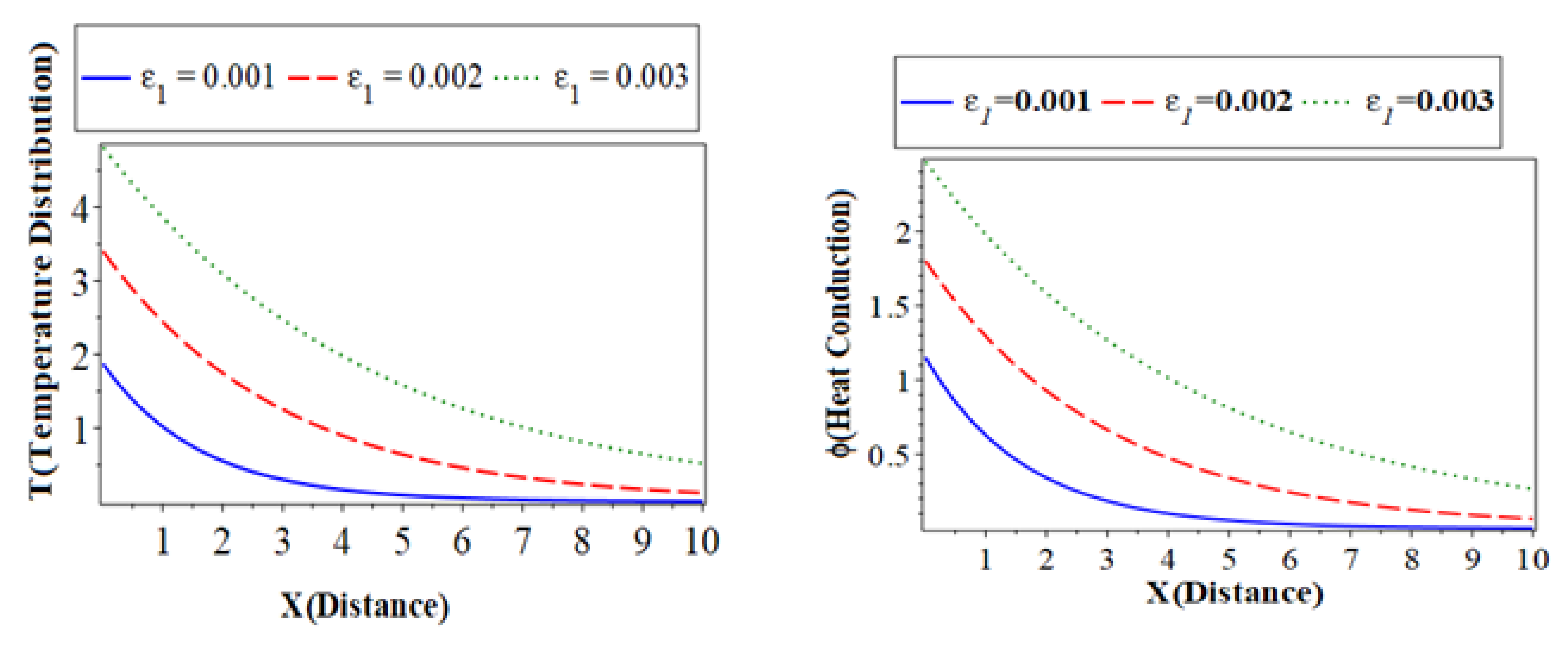The solid lines () with a blue color curve represent the case when ${\epsilon }_1=0.001$ the dashed lines () with red color curve express the case at ${\epsilon }_1=0.002$, and the dotted lines () with a green color curve show the case at ${\epsilon }_1=0.001$. The first subfigure represents the temperature ($T$) distribution against the horizontal distance $x$ [30]. The temperature distribution starts from the maximum positive value for all three cases. In the case of ${\epsilon }_1=0.001$ the distribution takes on the exponential behavior with a smooth decrease. On the other hand, when ${\epsilon }_1=0.002$ and ${\epsilon }_1=0.003$ the distribution of displacement decreases sharply in the first range; it takes on exponential propagation behavior until it reaches a minimum value near the zero line for the rough surface. The second subfigure displays the conduction heat ($\varphi$) distribution with the distance $x$, which takes on the same behavior as the first subfigure in the first category. The third subfigure displays the carrier density distribution against the distance in variation values of the thermoelastic parameter. However, a small change in thermoelastic coupling parameters has no significant effect on the carrier density, which has a similar quality behavior. The fourth subfigure describes the hole charge density with the distance. This subfigure shows that the amplitude values of the heat conduction distribution increase with the decrease in the values of the thermoelastic coupling parameters due to acceleration of thermal waves and photothermal excitation. The fifth subfigure displays the increases of stress force $\sigma$ amplitude, due to the mechanical loads, tends to increase the value of thermoelastic coupling parameters. The sixth subfigure displays the displacement $u$ distributions against the distance x which show that the curves are carried out from the negative value approach to zero at all cases. On the other hand, all the physical quantities under study are affected by changes in the thermoelastic coupling parameter. This is because the absolute value of the main fields is very sensitive to the changes of the thermoelastic coupling parameter.

6.3. The Effect of the Phase-Lag of the Temperature Gradient

Figure 2 (which represents the second category) shows the main physical fields against the horizontal distance $x$ with electron and hole constants. All calculations are carried out when ${\epsilon }_1=0.001$ and ${\tau }_q=1$ in the context of a hyperbolic two-temperature process for Silicon (Si) material. All subfigures discuss three cases of the phase-lag of the temperature gradient. 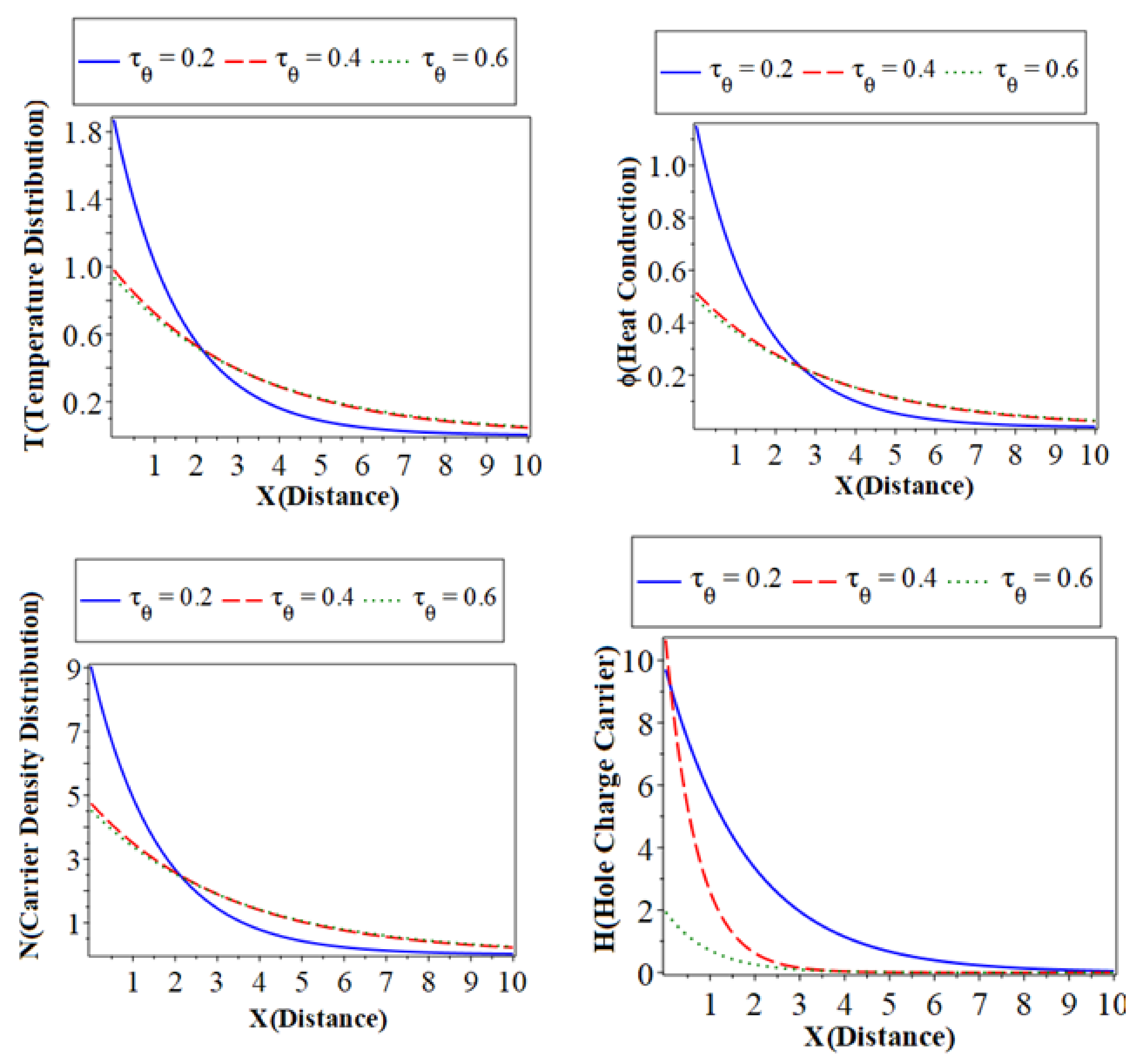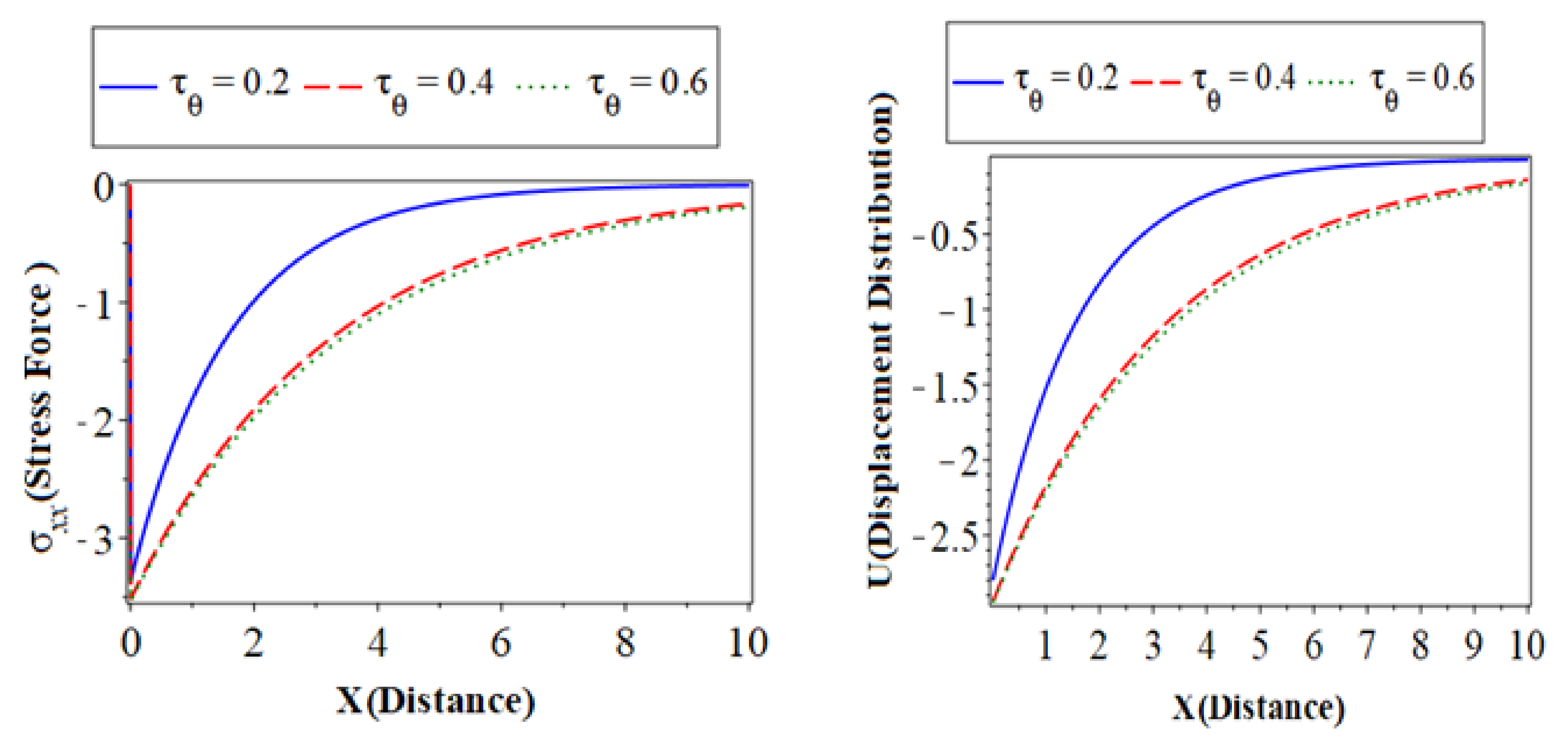The solid lines () with a blue color curve represent the case when ${\tau }_{\theta }=0.6$,the dashed lines () with red color curve express the case at ${\tau }_{\theta }=0.4$ and the dotted lines () with a green color curve show the case at ${\tau }_{\theta }=0.2$.The first subfigure displays the temperature ($T$) distribution with the distance $x$. It takes on the same behavior of the temperature distribution in the above subfigure for the thermoelastic coupling parameters $\varphi$ and $x$ that has the same behavior of temperature distribution. The third describes the carrier density distribution $N$ against the distance $x$ in variation values of the phase-lags of the temperature gradients that have the same behavior of temperature distribution and heat conduction. The fourth subfigure displays the hole charge carrier to increase the value of thermoelastic coupling parameters. The fifth subfigure displays that the increase of $\sigma$ amplitude, due to the mechanical loads, tends to increase the value of the phase-lag of the temperature gradients. The sixth subfigure represents the $u$ distribution against the horizontal distance $x$ ${\tau }_{\theta }=0.2$ the distribution takes on the exponential behavior with a smooth increase. When ${\tau }_{\theta }=0.4$ and ${\tau }_{\theta }=0.6$ the distribution of displacement increases sharply in the first range; it takes on exponential propagation behavior until it reaches a minimum value near the zero line. The values of the examined fields grow as the phase-lags of the temperature gradients‘ value decreases; this can be seen from the curves’ behavior.

6.4. The Effect of the Phase-Lag of the Heat Flux

Figure 3 (which represents the third category) shows the main physical fields against the horizontal distance $x$ with electron and hole constants. All calculations are carried out under the effect of the external magnetic field when ${\epsilon }_1=0.001$ in the context of a hyperbolic two-temperature process for silicon (Si) material. All subfigures discuss three cases of the phase-lag of the heat flux parameter. The solid lines () with a blue color curve represent the case when ${\tau }_q=3$ the dashed lines () with red color curve express the case at ${\tau }_q=2$ and the dotted lines () with a green color curve show the case at ${\tau }_q=1$. The first, second, and third subfigures are the temperature ($T$) distribution, heat conduction, and the carrier density distribution with the distance $x$, which takes on the same behavior as the first category. The fourth subfigure describes the hole charge carrier with the distance. This subfigure shows that the amplitude values of the hole charge carrier distribution increase with the decrease in the values of the thermoelastic. The fifth subfigure shows that the increase of stress force $\sigma$ amplitude, due to the mechanical loads, tends to increase the value of the phase-lag of the heat fluxes. The sixth subfigure represents the wave propagation of displacement $u$ distribution against the horizontal distance $x$. The displacement distribution starts from the maximum positive value for all three cases. In the case of ${\tau }_q=2$ the distribution takes on the exponential behavior with a smooth decrease. On the other hand, when ${\epsilon }_1=0.001$ the distribution of displacement decreases sharply in the first range, and it takes on exponential propagation behavior until it reaches a minimum value near the zero line [31]. The numerical results show that each field of physical quantities is significantly influenced by the phase-lag of the heat flux [32].

6.5. The Effect of the Hyperbolic Two-Temperature

Figure 4 (which represents the third category) shows the main physical fields against the horizontal distance $x$ with electron and hole constants. All calculations are carried out under the effect of the external magnetic field when ${\epsilon }_1=0.001$ in the context of a hyperbolic two-temperature process for silicon (Si) material. All subfigures discuss three cases of the hyperbolic two-temperature parameter. The solid lines () with a blue color curve represent the case when ${\tau }_q=3$ the dashed lines () with red color curve express the case at ${\tau }_q=2$ and the dotted lines () with a green color curve show the case at ${\tau }_q=1$. The first subfigure shows temperature ($T$) distribution. The second subfigure displays the heat conduction, and the third subfigure displays the carrier density distribution against the distance $x$ in variation values of the hyperbolic two-temperature parameters, which take the same behavior in the first category. The fourth subfigure describes the hole charge carrier with the distance. The fifth subfigure displays the increase of stress force $\sigma$ amplitude, due to the mechanical loads, that tend to increase the value of the phase-lag of the heat fluxes. The sixth subfigure represents the wave propagation of displacement $u$ distribution against the horizontal distance $x$. The displacement distribution starts from the minimum negative value for all three cases. It takes on exponential propagation behavior until it reaches a maximum value near the zero line [33,34]. It is evident that the propagation of the photo-thermal waves within the semiconductor media is reduced by the increase in the hyperbolic two-temperature parameter. Additionally, the significance of the suggested version is demonstrated by contrasting the outcomes of the current framework with those in the case of the hyperbolic two-temperature theory. This is because the issue of heat waves traveling at infinite speeds has been resolved.

6.6. The Comparison between Si and Ge Materials

Figure 5 (the fifth category) illustrates the comparison between the elastic semiconductor materials Silicon (Si) and germanium (Ge) in the context of the hyperbolic two-temperature process. In this category, the values of the physical fields under study are evaluated numerically when ${\epsilon }_1=0.001$ ${\tau }_q=1,\beta =1$ and ${\tau }_{\theta }=0.2$ under the influence of the hole charge carrier. From this figure, there is a clear difference in the physical constant values of Ge and Si materials; they have a great effect on all the wave propagation of the dimensionless distributions for $T$, $u$, $H$, $\sigma$, $\varphi$ and $N$ [31].

7. Conclusions

In the context of photo-thermoelasticity theory, the primary goal of this work is to investigate the dynamics of a two-dimensional elastic media semiconductor during processes involving holes/electrons under the influence of the hyperbolic two-temperature theory. The fundamental issue is resolved using the Laplace transform and Fourier transform techniques. In order to carry out the numerical estimations for significant physical quantities, these equations’ solutions are seen under the inversion of numerical integral transformations according to specified boundary loads. The thermoelastic coupling parameters, electronic and thermal relaxation times, the hyperbolic two-temperature, and physical constants of the medium play a significant role in all the physical distributions. The problem is helpful for scientists and engineers who work in renewable energy. Many applications in electronics manufacturing, such as geophysics, airplane, and solar cells would benefit from understanding this problem. The investigation in this paper has wide application in material science, engineering problems, thermodynamics, and thermoelasticity. In addition, it is beneficial for researchers.

References

- Rayleigh, L. On waves propagated along the plane surface of an elastic solid. Proc. Lond. Math. Soc. 1885, 1, 4–11. [Google Scholar] [CrossRef]
- Lockett, F.J. Effect of thermal properties of a solid on the velocity of Rayleigh waves. J. Mech. Phys. Solids 1958, 7, 71–75. [Google Scholar] [CrossRef]
- Chandrasekharaiah, D.S. Hyperbolic Thermoelasticity: A review of recent literature. Appl. Mech. Rev. 1998, 51, 705–729. [Google Scholar] [CrossRef]
- Maruszewski, B. Electro-magneto-thermo-elasticity of Extrinsic Semiconductors, Extended Irreversible Thermodynamic Approach. Arch. Mech. 1986, 38, 83–95. [Google Scholar]
- Sharma, J.; Thakur, N. Plane harmonic elasto-thermodiffusive waves in semiconductor materials. J. Mech. Mater. Struct. 2006, 1, 813–835. [Google Scholar] [CrossRef]
- Sharma, J.N.; Thakur, N.; Singh, S. Propagation Characteristics of Elasto-Thermodiffusive Surface Waves in Semiconductor Material Half-Space. J. Therm. Stress. 2007, 30, 357–380. [Google Scholar] [CrossRef]
- Lotfy, K.; El-Bary, A. Elastic-thermal-diffusion model with a mechanical ramp type and variable thermal conductivity of electrons–holes semiconductor interaction. Waves Random Complex Media 2022. [Google Scholar] [CrossRef]
- Aldwoah, K.; Lotfy, K.; Mhemdi, A.; El-Bary, A. A novel magneto-photo-elasto-thermodiffusion electrons-holes model of excited semiconductor. Case Stud. Therm. Eng. 2022, 32, 101877. [Google Scholar] [CrossRef]
- Hobiny, A.; Abbas, I. Generalized Thermo-Diffusion Interaction in an Elastic Medium under Temperature Dependent Diffusivity and Thermal Conductivity. Mathematics 2022, 10, 2773. [Google Scholar] [CrossRef]
- Abouelregal, A.E.; Sedighi, H.M.; Shirazi, A.H. The Effect of Excess Carrier on a Semiconducting Semi-Infinite Medium Subject to a Normal Force by Means of Green and Naghdi Approach. Silicon 2021, 14, 4955–4967. [Google Scholar] [CrossRef]
- Awwad, E.; Abouelregal, A.E.; Atta, D.; Sedighi, H.M. Photo-thermoelastic behavior of a functionally graded? Semiconductor medium excited by thermal laser pulses. Phys. Scr. 2022, 97, 030008. [Google Scholar] [CrossRef]
- Nayfeh, A.H.; Nemat-Nasser, S. Transient thermoelastic waves in half-space with thermal relaxation. Z. Angew. Math. Phys. 1972, 23, 52–68. [Google Scholar] [CrossRef]
- Chen, P.J.; Gurtin, M.E.; Williams, W.O. On the thermodynamics of non- simple elastic materials with two temperatures. Z. Angew. Math. Phys. 1969, 20, 107–112. [Google Scholar] [CrossRef]
- Chen, J.; Beraun, J.; Tham, C. Ultrafast thermoelasticity for short-pulse laser heating. Int. J. Eng. Sci. 2004, 42, 793–807. [Google Scholar] [CrossRef]
- Quintanilla, T.; Tien, C. Heat transfer mechanism during short-pulse laser heating of metals. ASME J. Heat Transf. 1993, 115, 835–841. [Google Scholar]
- Youssef, H. Theory of two-temperature-generalized thermoelasticity. IMA J. Appl. Math. 2006, 71, 383–390. [Google Scholar] [CrossRef]
- Youssef, H.M. Theory of Two-Temperature Thermoelasticity without Energy Dissipation. J. Therm. Stress. 2011, 34, 138–146. [Google Scholar] [CrossRef]
- Youssef, H.; El-Bary, A. Theory of hyperbolic two-temperature generalized thermoelasticity. Mater. Phys. Mechs. 2018, 40, 158–171. [Google Scholar]
- Lotfy, K.; Elidy, E.S.; Tantawi, R.S. Photothermal Excitation Process during Hyperbolic Two-Temperature Theory for Magneto-Thermo-Elastic Semiconducting Medium. Silicon 2021, 13, 2275–2288. [Google Scholar] [CrossRef]
- Lotfy, K.; Elidy, E.S.; Tantawi, R. Piezo-photothermoelasticity transport process for hyperbolic two temperature theory of semiconductor material. Int. J. Mod. Phys. C 2021, 32, 2150088. [Google Scholar] [CrossRef]
- Christofides, C.; Othonos, A.; Loizidou, E. Influence of temperature and modulation frequency on the thermal activation coupling term in laser photothermal theory. J. Appl. Phys. 2002, 92, 1280–1285. [Google Scholar] [CrossRef]
- Marin, M.; Florea, O. On Temporal Behaviour of Solutions in Thermoelasticity of Porous Micropolar Bodies. An. Univ. Ovidius Constanta 2014, 22, 169–188. [Google Scholar] [CrossRef]
- Abouelregal, A.E.; Marin, M. The Size-Dependent Thermoelastic Vibrations of Nanobeams Subjected to Harmonic Excitation and Rectified Sine Wave Heating. Mathematics 2020, 8, 1128. [Google Scholar] [CrossRef]
- Mahdy, A.M.S.; Lotfy, K.; Hassan, W.; El-Bary, A.A. Analytical solution of magneto-photothermal theory during variable thermal conductivity of a semiconductor material due to pulse heat flux and volumetric heat source. Waves Random Complex Media 2020, 31, 2040–2057. [Google Scholar] [CrossRef]
- Honig, G.; Hirdes, U. A method for the numerical inversion of Laplace transforms. J. Comput. Appl. Math. 1984, 10, 113–132. [Google Scholar] [CrossRef]
- Khamis, A.K.; Lotfy, K.; El-Bary, A.A.; Mahdy, A.M.S.; Ahmed, M.H. Thermal-piezoelectric problem of a semiconductor medium during photo-thermal excitation. Waves Random Complex Media 2020, 31, 2499–2513. [Google Scholar] [CrossRef]
- Yadav, A.K. Photothermal plasma wave in the theory of two-temperature with multi-phase-lag thermo-elasticity in the presence of magnetic field in a semiconductor with diffusion. Waves Random Complex Media 2020. [Google Scholar] [CrossRef]
- Mandelis, A.; Nestoros, M.; Christofides, C. Thermoelectronic-wave coupling in laser photothermal theory of semiconductors at elevated temperatures. Opt. Eng. 1997, 36, 459–468. [Google Scholar] [CrossRef]
- Todorović, D.; Nikolić, P.; Bojičić, A. Photoacoustic frequency transmission technique: Electronic deformation mechanism in semiconductors. J. Appl. Phys. 1999, 85, 7716–7726. [Google Scholar] [CrossRef]
- Abbas, I.A.; Alzahrani, F.S.; Elaiw, A. A DPL model of photothermal interaction in a semiconductor material. Waves Random Complex Media 2018, 29, 328–343. [Google Scholar] [CrossRef]
- Liu, J.; Han, M.; Wang, R.; Xu, S.; Wang, X. Photothermal phenomenon: Extended ideas for thermophysical properties characterization. J. Appl. Phys. 2022, 131, 065107. [Google Scholar] [CrossRef]
- Hobinya, A.; Abbas, I. A GN model on photothermal interactions in a two-dimensions semiconductor half space. Result. Phys. 2019, 15, 102588. [Google Scholar] [CrossRef]
- Mahdy, A.; Lotfy, K.; El-Bary, A.; Sarhan, H. Effect of rotation and magnetic field on a numerical-refined heat conduction in a semiconductor medium during photo-excitation processes. Eur. Phys. J. Plus. 2021, 136, 553–560. [Google Scholar] [CrossRef]
- Song, Y.; Todorovic, D.; Cretin, B.; Vairac, P. Study on the generalized thermoelastic vibration of the optically excited semiconducting microcantilevers. Int. J. Solids Struct. 2010, 47, 1871. [Google Scholar] [CrossRef]