Tutorial on Chemical Pressure Analysis: How Atomic Packing Drives Laves/Zintl Intergrowth in K₃Au₅Tl

Abstract

The tight atomic packing generally exhibited by alloys and intermetallics can create the impression of their being composed of hard spheres arranged to maximize their density. As such, the atomic size factor has historically been central to explanations of the structural chemistry of these systems. However, the role atomic size plays structurally has traditionally been inferred from empirical considerations. The recently developed DFT-Chemical Pressure (CP) analysis has opened a path to investigating these effects with theory. In this article, we provide a step-by-step tutorial on the DFT-CP method for non-specialists, along with advances in the approach that broaden its applicability. A new version of the CP software package is introduced, which features an interactive system that guides the user in preparing the necessary electronic structure data and generating the CP scheme, with the results being readily visualized with a web browser (and easily incorporated into websites). For demonstration purposes, we investigate the origins of the crystal structure of K₃Au₅Tl, which represents an intergrowth of Laves and Zintl phase domains. Here, CP analysis reveals that the intergrowth is supported by complementary CP features of NaTl-type KTl and MgCu₂-type KAu₂ phases. In this way, K₃Au₅Tl exemplifies how CP effects can drive the merging for geometrical motifs derived from different families of intermetallics through a mechanism referred to as epitaxial stabilization.

1. Introduction

Conflict between electronic and steric factors is a theme that pervades chemistry as a field. When such schemes are proposed for solid-state and materials systems, however, there is a large asymmetry in theoretical tools available for analyzing the two sides of this scheme. To explore the electronic factor, one can anticipate preferred electron counts based on the features of density of states (DOS) curves [1,2], quantify interaction strengths with the crystal orbital Hamiltonian population (COHP) analysis [3,4,5], detect regions of space where individual electron pairs tend to predominate with the electron localization function (ELF) [6,7,8], and generate localized orbitals from the wavefunctions using Wannier analysis [9,10,11,12,13] or the reverse approximation Molecular Orbital (raMO) approach [14,15]. Together, these and other methods provide a powerful theoretical toolbox for analyzing the ways in which the valence electrons of a system influence the stability of different crystal structure arrangements. The spatial requirements of the atoms, on the other hand, are more difficult to assess from electronic structure calculations, as atomic size is inherently an empirical concept rather than a fundamental feature of quantum mechanics. As such, the investigation and analysis of size effects has traditionally relied on considerations of atomic radii [16,17].

Recently, DFT Chemical Pressure (CP) analysis was developed as an approach to address this issue, with a particular interest in the structural chemistry of intermetallic phases [18,19,20,21,22,23]. This method is based on the recognition that non-optimal interatomic distances are detectable in the local pressures that surround the atoms of a solid-state lattice, as constructed from the output of DFT calculations. In the study of a variety of intermetallic phases, CP analysis has provided explanations for diverse structural phenomena, such as the insertion of interfaces into simple structures [19,20,24,25], the adoption of local icosahedral symmetry in quasicrystal approximants [26,27,28], the emergence in incommensurability [29,30,31,32,33,34], the stabilizing effects of various kinds of single point substitutions [23,24,25,35,36], and the formation of intergrowth structures [27,35,37,38,39]. The CP maps generated in the process can also be used to analyze the forces involved in chemical bonding and molecular structure [40,41,42,43].

Recent developments in the CP methodology have widened its applicability [18,19,20,21,22,23], opening the potential for it to serve as a tool for a larger portion of the solid-state and materials chemistry communities. With this goal in mind, we present here a tutorial on the CP method, illustrating how one goes from the Crystallographic Information File (CIF) [44] of a structure all the way to the creation and interpretation of its CP scheme. To demonstrate the procedure, we will explore the intermetallic phase K₃Au₅Tl (own type) discovered by Li et al. [45], and how it can be understood as an CP-driven intergrowth between a NaTl-type KTl phase and an MgCu₂-type KAu₂ phase (Figure 1). The K₃Au₅Tl phase is of particular interest because it can serve as a manifestation of CP that combines the structural motifs of two foundational families of solid-state compounds: the Zintl phases and the Laves phases represented by the NaTl and MgCu₂ structure types, respectively.

2. Overview of the CP Method

Let’s begin with an overview of the CP method and how it uncovers packing tensions within a crystal structure in terms of local interatomic pressures. The core of the CP approach is a simple implementation of the concepts of the quantum mechanical energy and stress densities [46,47,48,49,50]. Here, we recognize that major contributions to the Kohn–Sham total energy in a periodic DFT calculation can be represented as a sum over an energy grid, as in

$$E_{DFT}={\displaystyle \sum }_j{\rho }_{energy,j}{V}_{voxel}+E_{nonlocal}+E_{Ewald}+E_{\alpha }$$

(1)

where j indexes the voxels (the 3D analogs of pixels) into which the cell is divided, and ${\displaystyle \sum }_j{\rho }_{energy,j}{V}_{voxel}\approx {\iiint }_{cell}^{}{\rho }_{energy}\left(\stackrel{\rightharpoonup }{r}\right)dV$ includes the kinetic energy, the exchange-correlation energy, as well as the local pseudopotential and Hartree energies aside from the divergent Fourier components at the origin in reciprocal space, which are combined in a convergent way in the E_Ewald + E_α terms (see Ref. [51] and Section 6 for more detail). Finally, E_nonlocal is the energy contribution arising from the nonlocal operators in the pseudopotentials that capture the differential screening of electrons in states with s-, p-, d- and f-orbital character. Once such energy grids are constructed from the output of DFT calculations, the total pressure, P, of a structure can be resolved as an average over an analogous pressure grid:

$$P=\frac{1}{N_{voxels}}{{\displaystyle \sum }}_j{P}_{voxel,j}=-\frac{1}{N_{voxels}}{{\displaystyle \sum }}_j\frac{\partial E_{voxel,j}}{\partial V_{voxel}}+P_{remainder}$$

(2)

where N_voxels is the number of voxels into which the cell is divided, E_voxel,j is the energy associated with voxel j, V_voxel is the voxel volume, and P_remainder represents the contributions to the pressure from energy terms not simply amenable to spatial mapping (discussed at greater length below). In this way, the local responses to the compression or expansion of a structure can be spatially resolved. In practice, this procedure is carried out on a structure by calculating numerical derivatives using energy grids constructed at three slightly different volumes (the equilibrium volume, as well as expanded and contracted volumes).

Once the local pressure map is constructed, we interpret it in terms of interatomic interactions. While a number of ways for doing this have been devised [18,19], the most commonly used approach is known as the Hirshfeld-inspired contact volume scheme [20,21,22,23]. Here, following the Hirshfeld charge analysis [52], a hypothetical reference density (referred to as the pro-density) is constructed from the sums of the free atom electron densities (or free ion electron densities, if charges are assumed), with no interactions between the atoms. The relative contributions from each atom to the pressure at each point in space is then judged by the sizes of their contributions to the pro-density at that point. We then introduce a substantial simplification: we consider the pressure at each point as arising from the interaction between the two largest contributors, leading to a division of the unit cell into volumes corresponding to pairs of atoms. The contributions within these contact volumes are then averaged to create interatomic pressures. Finally, we can visualize the results by projecting the pressures onto atom-centered spherical harmonics and plotting the distributions. In the next sections, we will demonstrate these steps in detail as outlined in Figure 2, using the CP scheme of K₃Au₅Tl as a specific example.

3. Installation of the CP Software

For the following, we will need access to a PBS cluster (adaptations of the scripts for other queue systems are possible) for carrying out the DFT calculations and generating the CP schemes, as well as a local computer with a web browser for the visualization of the results. On the cluster, ABINIT (Ver. 7.10.5 for the current implementation) [53,54,55,56], the Atomic Pseudopotentials Engine [57], the Bader program (a freely available tool developed by Henkelman et al.) [58,59,60,61], and the GNU Scientific Library [62] should be installed. Next, the DFT-CP package can be downloaded from GitHub DFT-CP repository (URL: https://www.GitHub.com/Fredrickson-UW/DFT-CP/, accessed on 26 July 2021) and compiled according to the instructions provided, with a path being provided on the cluster to the executable files and the apeDEN_files directory in the repository being placed in the home directory of the user. In addition, the FigureToolWeb package should be copied to the local directory in which the CP results will be examined. More detailed information regarding the programs included in these packages are given in the Supplementary Materials.

Figure 2. Flow chart of steps involved in generating a CP scheme. In this chart, the arrows are labeled with the program(s) necessary for that step and the boxes show the output obtained by the steps. The relevant section of this tutorial for each step is indicated on the right.

Figure 2. Flow chart of steps involved in generating a CP scheme. In this chart, the arrows are labeled with the program(s) necessary for that step and the boxes show the output obtained by the steps. The relevant section of this tutorial for each step is indicated on the right.

4. Preparing the Input Data for CP Analysis

The first step in the CP analysis of K₃Au₅Tl is the generation of the necessary electronic structure data using a planewave DFT package, ABINIT. In this section, we will describe a streamlined process for setting up and running these ABINIT calculations beginning from a CIF file. This process involves three scripts to read in the CIF file for the structure of interest, then set up and submit the necessary jobs to the PBS queue: qabinit-k (k-point mesh convergence test), qabinit-opt (geometrical optimization) and qabinit-tryngfft (final single point calculations).

To begin the calculation, we start with the CIF file for K₃Au₅Tl, K3Au5Tl.cif, and set up our initial ABINIT input files configured for a k-point convergence test, with the command:

• $ qabinit-k -np 12 K3Au5Tl.files K3Au5Tl

where -np 12 indicates that 12 cores will be used for the ABINIT calculations, and K3Au5Tl is the base name for the files to be generated. Since no files from previous runs are present, the script prompts us to choose options for the file generation:

• BASE NAME: K3Au5Tl
• The file K3Au5Tl.in does not exist.
• This script will first generate .in file for the calculation.
• No previous -OPTIONS file exists. Will ask for the options below
• Do you wish to use the default settings for this calculation? [1=Yes] [2=No]

For most of the cases, using the default options for the calculation is sufficient, but if desired, four options can be changed manually at this stage: (1) whether ABINIT will convert to the primitive cell if the original unit cell has centering, (2) whether semicore pseudopotentials will be used, (3) how the k-point mesh will be specified, and (4) whether the calculation should include spin-orbit coupling. The defaults for these options are yes, no, (except for Group 11 and 12 elements, such as Au), Γ-centered grids, and no, respectively. The default use of the primitive unit cell conserves computational resources, but creates extra steps for the visualization of the results (see Section 8).

In the case of K₃Au₅Tl, the main factor that requires careful consideration is the spin orbit coupling, which can have significant effects for heavy elements such as Tl and Au [63]. For now, we will use the default setting with spin-orbit effects turned off until the optimization of the structure is complete. Later, we will manually turn on spin-orbit coupling at the single point calculation step. If we choose to set these parameters explicitly, we select Option 2 and then answer the prompts as follows:

• Please specify your settings for this calculation below.
• Do you want ABINIT to convert to a primitive cell if current one is centered? [1=Yes] [2=No] 1
• What kind of pseudopotential do you wish to use? [1=semicore only for 11 or 12 electron d-elements] [2=semicore when available] 1
• How do you want to specify your k-point mesh? [1=ngkpt] [2=kptrlatt] 1
• Do you want to enable spin orbit coupling? [1=No] [2=Yes] 1

From here, the program will read and process the CIF file:

• Full space group name: Imma
• Space group: 74
• Wyckoff position information found!
• Processing data for site 1.
• Processing data for site 2.
• Processing data for site 3.
• Processing data for site 4.
• Processing data for site 5.
• Processing data for site 6.
• There are 6 sites in total.
• Done processing CIF data.

After this step, the program writes and generates the ABINIT input files for LDA-DFT calculations employing Hartwigsen–Goedecker–Hutter norm-conserving pseudopotentials [64], and gives instructions for carrying out the calculation:

• Orthorhombic: I-centered
• Converting to primitive cell.
• Values of primitive cell vectors a, b and c: 11.076051 11.076051 11.076051 Angstroms
• Values of a*, b* and c*: 0.567277, 0.567277, 0.567277 1/Angstrom.

• Now writing the ABINIT .files file: K3Au5Tl.files ... Done.
• Now writing the ABINIT .in file: K3Au5Tl.in ... Done.

• ****************** NEXT STEPS ******************

• You chose automatic generation of the k-point mesh for the system.

• You chose to specify the k-point mesh with the ngkpt variable (default). The .in file has been populated with 5 choices. Some of these might be commented out for practical reasons. You may uncomment the ones you wish to include, adjusting ndtset accordingly.

• After you deal with any warnings below, you may submit your ABINIT job.

• Once the calculation is finished, you can find energy of different ngkpt grids by using [grep etotal “base name.log”]. You can then select a ngkpt grid based on this data, and update the abinit .in file with your choice for the future calculations. Convergence of the energy differences for different k-point meshes to lower than 5 meV/atom (0.00018 Ha/atom) is recommended.

• ****************** WARNINGS ******************

• There are no warnings! However, since this is a new calculation, it is still a good idea to carefully check the input file to be sure the CIF was properly read before you proceed.

• You may now submit your calculation.

• Make sure to carefully read the NEXT STEPS and WARNINGS before running ABINIT.
• This information is also available in the prepareABINIT-basename.log file.

Were we to choose to use non-default settings, such as kptrlatt, instead of ngkpt for specifying k-point mesh, the script would guide us through the available options and give further advice as applicable.

There are two warnings that are frequently encountered at this stage. First, for certain space groups more than one choice of origin is available. As the CIF file can be written in either, it will be necessary for the user to inspect the equivalent positions or open the CIF file in a visualization tool, such as Diamond [65] or VESTA [66,67], to determine which is used and manually set the value of the spgorig keyword in the ABINIT .in file. Another common warning arises when the CIF file contains a non-conventional orientation of the axes, as may happen in monoclinic and orthorhombic space groups. In such cases, the spgaxor keyword in the .in file should be adjusted according to the values given on the ABINIT space group help page (URL: https://docs.abinit.org/guide/spacegroup/, accessed on 26 July 2021). Other possible warnings and how to deal with them can also be found on the GitHub page.

After confirming that the ABINIT .in file has been properly populated with the data from the CIF file, we run the k-point mesh convergence calculation by simply rerunning qabinit-k:

• $ qabinit-k -np 12 K3Au5Tl.files K3Au5Tl

This time, the script will detect that the K3Au5Tl.files and K3Au5Tl.in already exist and will submit the calculation to the queue after receiving confirmation:

• ABINIT input files already exist.
• If there is a kmesh folder or ngkpt_ETOT file, this calculation will overwrite them.
• Press enter to submit the ABINIT calculation to the queue.

Once the calculation is complete, a new directory named kmesh under the original directory will be created for the files of the k-point mesh calculation stored in it; only files needed for future steps are copied to the original directory. If ngkpt is used to specify the k-point mesh, the original directory will also contain a file named ngkpt_ETOT_CONVERGENCE, which records the convergence details of the k-point mesh test. Otherwise, we can consult the .log file for the ABINIT calculation, which is kept in the original directory with the name K3Au5Tl_k.log. Based on the information in these files, a k-point mesh that gives good convergence of the total energy can be selected for the subsequent steps.

Now that the k-point mesh has been selected, the next step is the optimization of the geometry to remove any forces on the atoms not enforced by the constraints of the lattice. To do this, we switch to the script qabinit-opt, which has the same command line usage as qabinit-k:

• $ qabinit-opt -np 12 K3Au5Tl.files K3Au5Tl

qabinit-opt will determine that the ABINIT files for the geometry optimization have not been prepared and switch into the file generation mode, using the options it finds in the prepareABINIT-options-K3Au5Tl file created when we set up the previous calculation. We should tend to any warnings as we did for qabinit-k, and then edit the k-point mesh settings in the new ABINIT .in file in accordance with the results of the convergence test we performed previously. We can now submit the geometry optimization to the queue by running the qabinit-opt script again with

• $ qabinit-opt -np 12 K3Au5Tl.files K3Au5Tl

The calculation itself is a consecutive two-step geometry optimization: in the first step, the atomic positions are relaxed while the cell parameters are kept constant, which is followed by a full relaxation of the unit cell and atomic positions. As these steps are completed, two directories will be created, optcell0 and optcell2, containing the files generated by the optimizations. After these jobs are finished, the ABINIT .log files in these directories can be checked to make sure that convergence of the forces and stresses was achieved in each step.

Once the structure is optimized, the next part of the CP procedure is the calculation of ground state electronic structures at a series of unit cell volumes, with the updated K3Au5Tl.files and K3Au5Tl.in generated by the qabinit-opt serving as the basis. The ABINIT .in file is now configured for three separate single point calculations using the scalecart variable: one at a slightly expanded volume (V_eq⁺, scalecart1 3*1.005), one at the equilibrium volume (V_eq°, scalecart2 3*1.000), and one at a slightly contracted volume (V_eq^–, scalecart1 3*0.995). Moreover, to output the kinetic energy densities and components of the Kohn–Sham potentials needed for the generation of the CP maps, the ABINIT variables prtkden, prtpot, prtvha, prtvxc and prtvhxc are all set to 1.

Here, qabinit-opt also generates the input files for auxiliary CP calculations on extremely expanded (linear scale 120%; V_exp = 1.728 V_eq) and contracted (linear scale 80%; V_con = 0.512 V_eq) structures, which will be used in the treatment of the E_Ewald + E_α energy terms (see Section 6). The input files for these calculations are created in directories named expanded and contracted, with the ABINIT .files files being named K3Au5Tl_exp.files and K3Au5Tl_con.files, respectively. The ABINIT .in files, meanwhile, contain only one change relative to that for the equilibrium volume: the three scalecart keywords are set as scalecart1 3*1.205, scalecart2 3*1.200, and scalecart3 3*1.195 for the expanded volume, and scalecart1 3*0.805, scalecart2 3*0.800, and scalecart3 3*0.795 for the contracted volume.

At this point, other options can be specified in the .in files. For example, to turn on spin-orbit coupling, we change nspinor to 2 in the K3Au5Tl.in files and increase nband by the number of valence electrons in the unit cell.

A keyword that requires particular attention for this step is ngfft, which specifies the fast Fourier transform (FFT) grid for going between the reciprocal and real space representations of the potentials and electron density. Since there are three datasets, there will be three FFT grids to consider. Normally, these grids can be determined internally by ABINIT. However, for the CP analysis, it is important that the basis vectors be divided into the same number of grid points for the three datasets so that numerical derivatives can be easily calculated. In addition, for the symmetrization procedures in the CP program, it is often necessary for the number of grid points along each basis vector to be divisible by the denominators of any fractions that appear in the symmetry operations for the space group. Such issues can be avoided by making the ngfft parameters multiples of 12 when feasible.

The qabinit-tryngfft script is designed to assist in finding acceptable FFT grids that meet these requirements. We begin the calculation for K₃Au₅Tl the equilibrium volume by running the command

• $ qabinit-tryngfft -np 12 K3Au5Tl 1 1 1

where the three integers refer to the numbers of fast Fourier transform grid points that the three basis vectors will be divided into. The use of 1′s here directs the program to try submitting the job and let ABINIT choose the grids. In this case, the result is as follows:

• $ qabinit-tryngfft K3Au5Tl 1 1 1
• Queue: default
• Number of processors: 1
• ngfft [1]: 1
• ngfft[2]: 1
• ngfft[3]: 1
• LOG_FILE NAME: K3Au5Tl.log
• File K3Au5Tl.files found!
• Files file: K3Au5Tl.files
• Job ID is: 3862899
• For input ecut= 3.500000E+01 best grid ngfft= 162 162 162
• For input ecut= 3.500000E+01 best grid ngfft= 162 162 162
• For input ecut= 3.500000E+01 best grid ngfft= 160 160 160
• ngfft1 162 162 162
• ngfft2 162 162 162
• ngfft3 160 160 160
• getcut: wavevector= 0.0000 0.0000 0.0000 ngfft= 162 162 162
• getcut: wavevector= 0.0000 0.0000 0.0000 ngfft= 162 162 162
• 2
• ngfft not accepted
• ngfft_status is: 2
• ngfft not accepted. Please try another ngfft

ABINIT’s default FFT grids for the slightly expanded, equilibrium, and slightly contracted datasets in this case are 162 × 162 × 162, 162 × 162 × 162, and 160 × 160 × 160, respectively. These choices will not be suitable for CP analysis as they are not identical across the three datasets, and the values are not multiples of 12. After detecting this incompatibility, qabinit-tryngfft terminated the ABINIT job and notified us that adjustments to the FFT grid are needed.

To solve this issue, we rerun qabinit-tryngfft with specific choices for the three integers giving the FFT grid:

• $ qabinit-tryngfft -np 12 K3Au5Tl 180 180 180

where we have requested a 180 × 180 × 180 grid to maintain the relative proportions of the ABINIT recommendations, while gaining a little extra fineness (it is important to go up rather than down) and having all three numbers be multiples of 12. This time, the output is:

• $ qabinit-tryngfft K3Au5Tl 180 180 180
• Queue: default
• Number of processors: 1
• ngfft[1]: 180
• ngfft[2]: 180
• ngfft[3]: 180
• LOG_FILE NAME: K3Au5Tl.log
• File K3Au5Tl.files found!
• Files file: K3Au5Tl.files
• Job ID is: 3862901
• For input ecut= 3.500000E+01 best grid ngfft= 162 162 162
• input values of ngfft(1) =180 ngfft(2) =180 ngfft(3) =180 are alright and will be used
• For input ecut= 3.500000E+01 best grid ngfft= 162 162 162
• input values of ngfft(1) =180 ngfft(2) =180 ngfft(3) =180 are alright and will be used
• For input ecut= 3.500000E+01 best grid ngfft= 160 160 160
• input values of ngfft(1) =180 ngfft(2) =180 ngfft(3) =180 are alright and will be used
• ngfft 180 180 180
• getcut: wavevector= 0.0000 0.0000 0.0000 ngfft= 180 180 180
• getcut: wavevector= 0.0000 0.0000 0.0000 ngfft= 180 180 180
• 1
• ngfft accepted
• Now running ABINIT calculation
• After this calculation is completed, you should run qnonloc_k followed by qMerge to partition nonlocal energy.
• And then, run qBader to process the calculation outputs and prepare for APE calculations.

As shown in the output, the ABINIT program has adopted this grid and, as a result, qabinit-tryngfft will allow the ABINIT calculation to go forward.

To carry out the corresponding ABINIT calculations for the extremely expanded and contracted geometries, we go to the expanded and contracted directories and use qabinit-tryngfft as before:

• $ qabinit-tryngfft -np 12 K3Au5Tl 1 1 1

There is no change in the command because the script will identify the correct ABINIT .files file from the provided base name, in this case, K3Au5Tl.

After the completion of the single point calculations on both the expanded and the contracted volumes with appropriate FFT grids, we have finished all the required ABINIT calculations for the CP analysis. In summary, the process of creating the necessary ABINIT output for the CP analysis can be reduced to the application of three scripts: qabinit-k, qabinit-opt and qabinit-tryngfft. The first reads the CIF file and prepares k-point convergence tests. The second reads the CIF file, leads ABINIT through the optimization of the structure, and sets up input files for the final ABINIT calculations. Lastly, the third script assists in running the final calculations by checking that the FFT grids used will be amenable to CP analysis. The main user intervention required is to ensure that the geometrical parameters of the original CIF file are properly read, that the ABINIT steps converge properly, and that any warnings or advice generated are considered.

5. Initial Processing of the ABINIT Output

With all of the necessary planewave DFT calculations now complete, the next step in the CP procedure is to calculate several of the properties from the DFT output that will be used in the generation of the CP schemes: the atomic contributions to the nonlocal pseudopotential energies at the various volumes, the Bader atomic charges, and the Bader atomic volumes.

Let’s start with resolving the nonlocal pseudopotential energies into atomic contributions. As discussed in Ref. [23], this involves calculating the contributions to nonlocal energy from each atomic pseudopotential’s s-, p-, d- and f-type projectors. This calculation is particularly demanding, as it requires nested loops over k-points, bands, pairs of planewaves, the atoms, and non-local projectors. Taking our K₃Au₅Tl phase as an example, for the slightly expanded version of the primitive cell, there are 18 atoms, 8 symmetry-distinct k-points in the k-point mesh, 108 bands, and at least 28,000 planewaves at each k-point. As such, parallelization is important for all but the smallest systems.

For this reason, we supplied with the DFT-CP package a program that calculates the nonlocal energy contributions at individual k points¹ which can be run in a parallel batch fashion with the job submission script qnonloc_k. For example, for our model system K₃Au₅Tl, the jobs for the datasets centered on the equilibrium volume are submitted with

• $ qnonloc_k 8 K3Au5Tl.out K3Au5Tl

where the “8” indicates that there are eight symmetry-distinct k-points to be analyzed (as can be found by using the command grep nkpt K3Au5Tl.out). For each k-point, a log file will be written containing the nonlocal energy contributes for each atom. Once these are ready, the data for the k-points can be merged with the script qMerge:

• $ qMerge 8 K3Au5Tl.out K3Au5Tl

For each dataset, qMerge sums the data for the individual k-points into a single .log file and generates a 3D grid representing the distribution of the non-local energy throughout the crystal structure. This qnonloc_k + qMerge process should also be repeated for the auxiliary calculations in the expanded and contracted directories.

Let’s now move to determining the Bader charges and Bader atomic volumes for each atom for the equilibrium geometry and for the expanded and contracted versions. For all three, this process is carried out by running the qBader script with

• $ qBader K3Au5Tl.files K3Au5Tl

This script reads the electron density ABINIT output file and produces density files in the VASP CHGCAR format for the valence electron density (for compatibility with the Bader program) and an approximation to the full electron density constructed by adding in atomic core densities obtained from the Atomic Pseudopotentials Engine [57]. Then, the Bader program [58,59,60] is run using these files as input to determine the zero-flux surfaces separating atomic regions and integrate the electron density within the atomic volumes to obtain charges.

For the equilibrium geometry, we will also calculate the free-ion electron densities corresponding to various percentages of those Bader charges (or Mulliken or Löwdin charges obtained with the LOBSTER program [4,68,69] on PAW electronic structure results [70,71]; examples are given in the Supplementary Information) for the symmetry-distinct atoms in the structure for use in the Hirshfeld-inspired contact volume construction. Typically, this would involve densities corresponding to 25%, 50%, 75% and 100% of the Bader charges (as long as converged electronic structures of the isolated ions can be obtained), which will be used to explore how different assumptions about the degree of charge transfer between the elements influence the resulting CP scheme (in cases where there is a strong dependence of the results on the ionicity, comparisons with the phonon band structure can be helpful; see references [22,23]). This process is facilitated with the script prepareApe_shell, which reads the ACF.dat file output by Bader and prepares input files for the calculation of free-ion electronic structures with APE.

To run this script for K₃Au₅Tl, we type

• $ prepareApe_shell K3Au5Tl.files K3Au5Tl.out

where the two inputs are the .files and the .out files from the ABINIT calculation. As this script runs, it first reads in the fractional coordinates of the atoms and the symmetry operations of the crystal structure from the ABINIT output file. With this information, it will search through the list of atoms to determine which atoms are symmetrically equivalent to each other. After that, the charges on the atoms for each ionicity level are calculated according to the information in ACF.dat, with those on symmetrically equivalent atoms being averaged. These results are used to generate input files for the APE program and saved in new directories called ./Bader/I100, ./Bader/I75, ./Bader/I50, and ./Bader/I25, corresponding to the four different ionicity levels. Within each ionicity directory, there are then subdirectories for each symmetry-distinct atomic site (Au1, Au2, Au3, K1, K2, Tl1 for K₃Au₅Tl), which contain an APE input file (inp.ape) populated with the electron configuration corresponding to the specified charge on that site.

Some attention may be paid to the how the electron configurations are assigned here. For cationic atoms, the prepareApe_shell program takes electrons away from the occupied atomic orbital with the largest principal quantum number. For example, a Sc atom with a positive charge of 0.5 will only have 1.5 electron in its 4s shell and 1 electron untouched in the 3d shell. When considering an anion, the program will look to the electron configuration of the next element in the periodic table. For example, the ground state electron configuration for a Ru atom is [Kr]5s¹ 4d⁷. For Ru^0.5−, 0.5 extra electrons will be added to the 4d shell because the electron configuration of the next element in the periodic table, Rh, is [Kr]5s¹ 4d⁸. If other configurations are desired, the inp.ape files can be manually edited, though care should be taken when making such changes, as the interpretation of the CP scheme depends on the free ion densities being realistic.

When the inp.ape files are ready, the full series of APE calculations is carried out with the runApe script, which is simply run with

• $ runApe

runApe descends into each subdirectory and runs the APE calculations to get the density output files. It copies these density files into the home directory and renames them as Au1-100, Au2-100, Au3-100, K1-100, K2-100, Tl1-100, Au2-75, etc. Moreover, the header lines (first seven lines) of each APE density output file will be removed as they are not needed in the later steps. One issue that can arise here is that it may not be possible to obtain converged wavefunctions for some ions, particularly those with high negative charges, which will prompt runApe to issue a warning on the screen. We generally interpret this as reflecting an upper-bound on the ionicity that can be assumed for the system.

6. Calibrating the Localized Electron Count

We have now only one more preliminary step before we can move to generating the DFT-CP map: the treatment of the E_Ewald and E_α terms in the total energy. Together, these terms correspond to the energy of a system consisting of (1) the pseudopotential ion cores and (2) a homogeneous electron gas corresponding to the average valence electron density [51]. The uniform nature of the electron gas here makes it challenging to unambiguously resolve this energy spatially. One straightforward approach is to map these energies homogeneously. However, in practice we find that for pseudopotentials with core-like electrons included in the valence set, the E_Ewald + E_α contributions to the pressure can be so large that treating them homogeneously is problematic. The more subtle pressure features of atoms modelled with softer pseudopotentials can easily be overwhelmed in such cases. To overcome this difficulty, it is useful to partition the E_Ewald + E_α energy into contributions from more core-like electrons that are considered strongly bound to the ion cores (effectively cancelling some of the cores’ positive charges) and contributions from the remaining electrons that are considered delocalized for the purposes of mapping these terms [23]. The E_Ewald + E_α components from these localized and delocalized sets of electrons are then mapped to the atomic core regions and homogeneously through space, respectively.

The main challenge then becomes determining how many of the valence electrons each atom contributes to the system should be treated as localized. To accomplish this, we have developed a calibration procedure based on the idea that at extremely exaggerated volumes, we expect that the large internal pressures of the system should overwhelm local differences in the atomic pressures. Here, we use the results of the auxiliary calculations we performed in Section 4 on an extremely expanded and an extremely contracted structure. For the expanded unit cell, the localized electron count for each site is tuned so that all the atoms experience equal negative atomic CPs, while for the contracted unit cell, these localized counts are adjusted so that all atoms bear the same amount of positive CP. We have found that using an average of the localized electron counts for each atom in the expanded and contracted auxiliary CP calculations leads consistently to physically meaningful CP schemes for the equilibrium structure [25,36].

To implement this idea, we have included an automated calibration routine in CPpackage, the main DFT-CP program. The program starts with 0 localized electrons on all atomic sites, and then calculates the net atomic CP on each site (by integrating the CP map within atomic volumes derived in the Bader analysis; see Section 5). Once the CPs are calculated, the localized electron count on the site with the most negative CP will be kept at 0, while those on the other sites are increased based on their current CP using interpolation. Then, the CPs on each site are re-calculated from the list of newly generated localized electron counts, and these counts are adjusted accordingly. This process is repeated until the difference between the site with the largest CP and smallest CP reduces to less than 1%, which is set as the convergence threshold. After performing this calibration on both the expanded and contracted versions of the structure, we have two sets of localized electron counts, and can use the average for each site in the final CP calculation on the equilibrium volume.

To start this calibration process for our example system K₃Au₅Tl, we navigate to the expanded directory and use the command

• $ CPpackage K3Au5Tl.out K3Au5Tl_exp_cali

where the first input is the name of the ABINIT output file, and the second is the base name for the files CPpackage will generate.

CPpackage will first check for the existence of an .ini input file, in this case, K3Au5Tl_exp_cali.ini. After not finding it, the program creates an initial version of the .ini file populated with default values. A screenshot of this initial K3Au5Tl_exp_cali.ini file is shown in Figure 3. In this file, there are two areas where adjustments are needed: the CV_MODE (contact volume mode, boxed in red) and the ATOM_MODELS settings (boxed in blue). For our calibration process, we set the CV_MODE value to 6 to activate the automatic calibration of the localized electron counts². Next, we update the atom model settings to the appropriate values for this calculation. For example, for the gold sites, we set the free ion electron density file to Au-0 (a file generated by qBader, corresponding to a neutral Au atom), the semicore/valence-only flag to 1 to indicate we are using a semicore pseudopotential for Au, and the number of localized electrons to 0 since we are at the start of the calibration process. The template settings highlighted by the green box in Figure 3 do not require our attention at this stage but will be used later for the visualization of the CP scheme in Section 8.

After making these changes, we can again enter the command

• $ CPpackage K3Au5Tl.out K3Au5Tl_exp_cali

to carry out the calibration procedure. The program first runs several iterations of localized electron counts and outputs the following when convergence is reached:

• Atom 1 (Au) net pressure: -7.56 GPa
• Atom 2 (Au) net pressure: -7.56 GPa
• Atom 3 (Au) net pressure: -7.56 GPa
• Atom 4 (Tl) net pressure: -7.58 GPa
• Atom 5 (K) net pressure: -7.57 GPa
• Atom 6 (K) net pressure: -7.58 GPa
• Atom 7 (Au) net pressure: -7.56 GPa
• Atom 8 (Au) net pressure: -7.56 GPa
• Atom 9 (Au) net pressure: -7.56 GPa
• Atom 10 (K) net pressure: -7.57 GPa
• Atom 11 (Au) net pressure: -7.56 GPa
• Atom 12 (Tl) net pressure: -7.58 GPa
• Atom 13 (K) net pressure: -7.57 GPa
• Atom 14 (K) net pressure: -7.58 GPa
• Atom 15 (Au) net pressure: -7.56 GPa
• Atom 16 (K) net pressure: -7.57 GPa
• Atom 17 (Au) net pressure: -7.56 GPa
• Atom 18 (Au) net pressure: -7.56 GPa
• Percent difference in pressures is 0.313244 %
• CONVERGENCE REACHED! All pressures are within 0.313244 percent of the smallest pressure
• Localized electron counts are as follows:
• Site 0: 5.037840 localized electrons
• Site 1: 3.661721 localized electrons
• Site 2: 3.730546 localized electrons
• Site 3: 1.238634 localized electrons
• Site 4: -0.000000 localized electrons
• Site 5: 0.221567 localized electrons
• Site 6: 5.037840 localized electrons
• Site 7: 3.661721 localized electrons
• Site 8: 3.730546 localized electrons
• Site 9: -0.000000 localized electrons
• Site 10: 5.037840 localized electrons
• Site 11: 1.238634 localized electrons
• Site 12: 0.000000 localized electrons
• Site 13: 0.221567 localized electrons
• Site 14: 5.037840 localized electrons
• Site 15: 0.000000 localized electrons
• Site 16: 3.661721 localized electrons
• Site 17: 3.661721 localized electrons

From the screen output, we can confirm that the final pressures are very close to each other, and negative in accordance with the unit cell being expanded relative to the equilibrium geometry. In the last section of the screen output, the calibrated localized electron counts for the sites are listed. If we repeat the same calculation for the contracted structure, we will have a complete list of calibrated localized electron counts for both the expanded and contracted versions of structure, as shown in

Table 1. Localized electron calibration result for K₃Au₅Tl at expanded volume.

	Site	Initial CP (GPa)	Localized Electron Count	Final CP (GPa)
Expanded	Au1	211.38	5.038	−7.56
	Au2	12.97	3.662	−7.56
	Au3	11.56	3.731	−7.56
	K1	−235.32	0.000	−7.57
	K2	−212.27	0.222	−7.58
	Tl1	−119.80	1.238	−7.58
Contracted	Au1	1067.01	2.497	195.51
	Au2	44.41	1.117	195.46
	Au3	55.68	1.141	195.45
	K1	−414.53	0.000	195.48
	K2	7.30	0.865	195.50
	Tl1	−7.06	0.746	195.50

. We can average them to find the localized electron counts that will be used in calculating the CP scheme at the equilibrium geometry (

Table 2. Calibrated localized electron counts for K₃Au₅Tl.

Site	Localized Electron Count
Au1	3.767
Au2	2.390
Au3	2.436
K1	0.000
K2	0.543
Tl1	0.992

).

7. Obtaining the CP Scheme

After performing the above preliminary steps, we are at last ready to generate and visualize the structure’s CP scheme. In the main directory, we invoke CPpackage again:

• $ CPpackage K3Au5Tl.out K3Au5Tl_I0

where we have chosen the base name for CP output as K3Au5Tl_I0 to indicate that this will be a 0% ionicity calculation (i.e., assuming all atoms have neutral charges for the purposes of the Hirshfeld-inspired contact volume construction). This step will generate the K3Au5Tl_I0.ini file, which we edit so that the CV_MODE is set to 0 (default), the pseudopotential options are given appropriately, and the localized electron count for each atomic site corresponds to the values obtained in our calibration. Next, we start the calculation of the CP scheme by re-typing the command

• $ CPpackage K3Au5Tl.out K3Au5Tl_I0

The CPpackage step will write eight output files in total, e.g., K3Au5Tl_I0-cell, K3Au5Tl_I0-geo, K3Au5Tl_I0-coeff, K3Au5Tl_I0-cplog, K3Au5Tl_I0-CP.xsf, K3Au5Tl_I0-averaged.xsf, K3Au5Tl_I0.js and K3Au5Tl_I0.html. Among them, the -cell and -geo files record the cell parameters and the atomic positions, the -coeff contains the projections of the interatomic pressures onto atom-centered spherical harmonics, and the –cplog file records the details and screen output of the CP calculation. The two .xsf files contain the volumetric data for the CP map, with the –CP.xsf and –averaged.xsf files showing the CP map before and after the averaging within contact volumes. These can be visualized in XCrysDen [72,73] or VESTA [66,67]. To view the integrated and projected CP scheme, we use the .js and .html files, as well as our FigureToolWeb library, as described in Section 8.

Generally, we will also want to generate CP schemes at other ionicity values to test how the results depend on this parameter. For this, we only need to change the file names for the free ion electron densities generated with APE in the .ini file accordingly. For example, to calculate the 25% CP scheme, we start a new calculation with the root name K3Au5Tl_I25, change the name of the Au1 site profile from Au1-0 to Au1-25 and all other sites accordingly in the .ini file, and then run CPpackage again.

8. Visualizing the CP Scheme

To view the CP scheme obtained through the above steps, we simply copy the .js and .html files created by CPpackage to a local directory, along with the contents of the FigureToolWeb package (available on the DFT-CP GitHub page; see Section 3), which utilizes three.js (URL: https://threejs.org/, accessed on 26 July 2021) to create 3D interactive models of crystal structures and theoretical data. 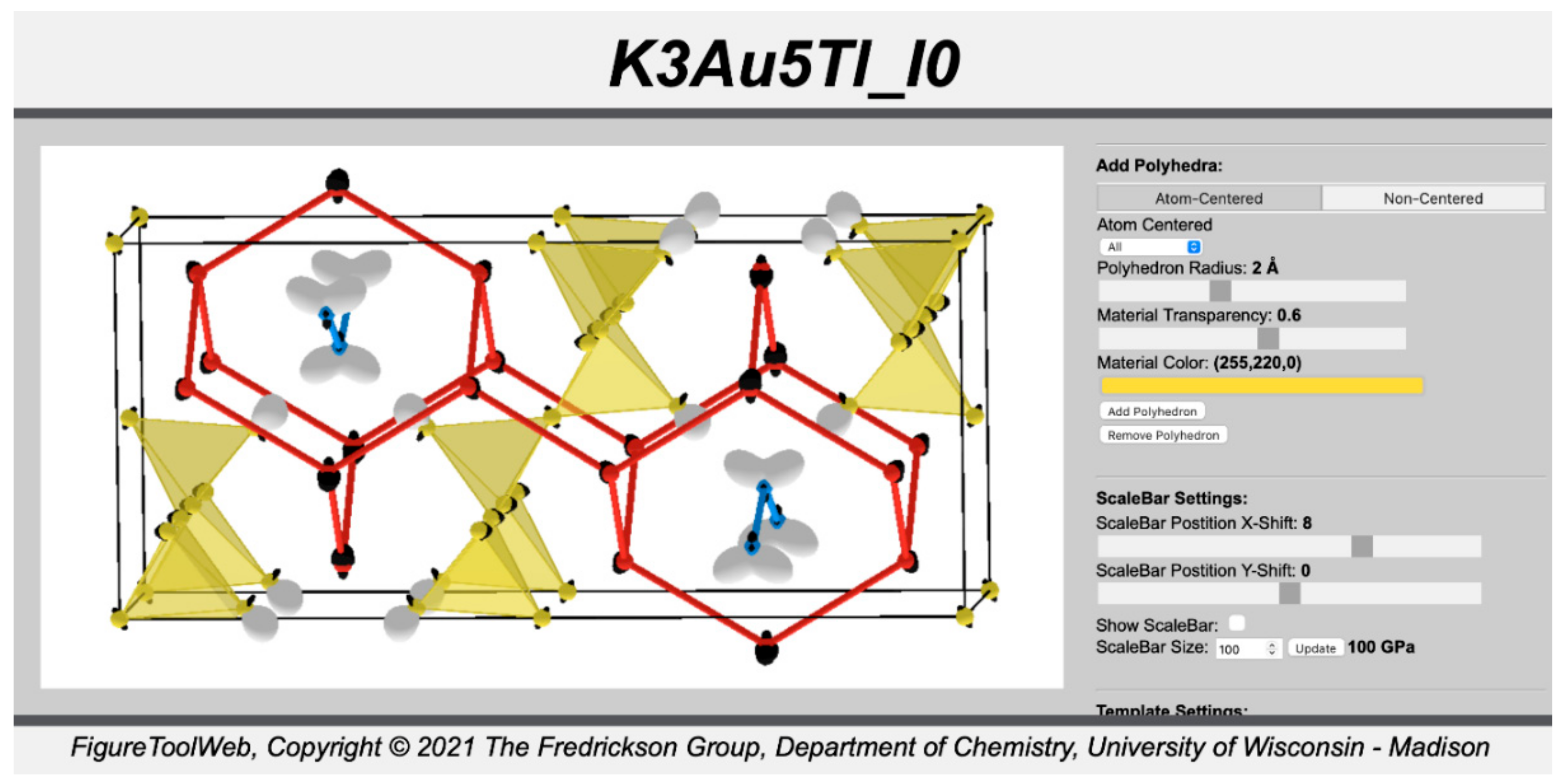Loading the .html file in your web browser will then show the CP scheme overlaid on the contents of the unit cell used in the calculation, along with various tools for adjusting the picture placed in a panel on the right, as seen in Figure 4. The CP distribution around each atom is here represented with a radial plot, with the distance of the surface from the atomic center being proportional to the magnitude of the sum of the CP contributions along that direction. The sign of the pressure is given by the color: white for positive CP (indicating that the atoms are too close to each other and expansion is locally favorable), black for negative CP (indicating that the atoms are too far from each other and contraction is favorable).

Generally, the default representation of the geometry will be far from optimal for seeing how these CP features relate to the structure, especially when ABINIT has adopted a primitive cell (as is the case here). For this reason, we have introduced a number of features and options to give the user control over how the structure and CP data are presented. To begin with, the user has the option of providing customized templates containing the positions of the atoms which will be shown. All one has to do is load any of the .xsf files generated for the equilibrium geometry into a crystallographic visualization program such as VESTA, isolate the atoms desired for each template, save the geometries as .xtl files, place these files in the ABINIT working directory, and make a few modifications to the .ini file. For example, if we export two templates for K₃Au₅Tl named K3Au5Tl_CPtemp.xtl and K3Au5Tl_CPtemp2.xtl, we would adjust the TEMPLATES block of the .ini file to:

• TEMPLATES 2; number of template .xtl files provided as list below.
• K3Au5Tl_cptemp.xtl
• K3Au5Tl_cptemp2.xtl

These templates will be incorporated into the .js and .html files upon running CPpackage.

In addition to the possibility of supplying user-generated templates, several other visualization options are automatically incorporated into the .html file. In Figure 5, Figure 6, Figure 7, Figure 8, Figure 9 and Figure 10, we demonstrate some of them for the CP scheme of K₃Au₅Tl, using a template consisting of a full conventional cell and some strategically chosen atoms outside of the cell. We begin in Figure 5 with the CP scheme plotted on our template with default colors, connection lengths, and CP plotting options.

A notable geometrical element missing here is the outline of the unit cell for the structure. If desired, the cell can be drawn by first adding placeholder ‘Xe’ atoms to the JavaScript file at the corners of the chosen unit cell in the atom list of a new template. We then follow this with a small fragment of code to draw connections between the placeholder atoms with commands available in the FigureToolWeb library:

• var template3 = [];
• template3[0]=[‘Xe’, -2.67577, 9.38614, 4.16768];
• template3[1]=[‘Xe’, -2.67577, 9.38614, -4.16768];
• template3[2]=[‘Xe’, -2.67577, -9.38614, 4.16768];
• template3[3]=[‘Xe’, -2.67577, -9.38614, -4.16768];
• template3[4]=[‘Xe’, 2.67577, 9.38614, 4.16768];
• template3[5]=[‘Xe’, 2.67577, 9.38614, -4.16768];
• template3[6]=[‘Xe’, 2.67577, -9.38614, 4.16768];
• template3[7]=[‘Xe’, 2.67577, -9.38614, -4.16768];

• var cell_material = define_material({ color: “rgb(0,0,0)”},1);

• var cell1 = drawbonds_cylinder(template3,’Xe’,cell_material,’Xe’,cell_material,5.3,9,0.03);
• var cell2 = drawbonds_cylinder(template3,’Xe’,cell_material,’Xe’,cell_material,18,19,0.03);

• //Optional code for creating toggle box for unit cell
• dontshow_objects(cell1);
• dontshow_objects(cell2);
• var cellstat = 1;
• var toggcell = document.getElementById(“toggcell”);
• toggcell.onclick = function() {
•  if (cellstat===0) {
•    dontshow_objects(cell1);
•    dontshow_objects(cell2);
•    cellstat = 1;
•  }
•  else {
•    show_objects(cell1);
•    show_objects(cell2);
•    cellstat = 0
•  }
• }

The result is shown in Figure 6.

Next, under the Connection Settings options, we can adjust the distance limits for drawing connections between pairs of atoms, and toggle off connections we do not want to draw attention to. In this case, we increase this distance cut-off for the K-K contacts until the diamond network they form is visible. We do the same of the Au-Au contacts until the edges of the Au₄ tetrahedra appear. As in Figure 1, we also turn off the plotting of the Au-K and K-Tl contacts for clarity. Finally, under the cylinder thickness tab, we can emphasize the K and Tl sublattices by increasing their cylinder radii and enhance their contrast with the Au framework by decreasing the thickness of the Au-Au connectors. The resulting image is presented in Figure 7. While the radii of the spheres representing the atomic positions were kept at the defaults, they can also be adjusted or turned off.

These steps have reproduced much of the representation of the structure shown in Figure 1. However, the color schemes still do not match. To reconcile this, the color of each element can be changed independently under ATOM SETTINGS, leading to the image shown in Figure 8. Note that the connections are always drawn using the same colors as the corresponding atoms they connect; currently, the cylinder colors cannot be adjusted independently with the tool bars.

As a final step to representing the structure, the three-dimensional nature of the atomic arrangement can be highlighted by drawing a selection of polyhedra. Two methods are available here. FigureToolWeb allows the user to build polyhedra by selecting vertices from a list of symmetry inequivalent sites, or by the central atoms around which a polyhedron will be created. In the case of K₃Au₅Tl, we find that filling in the Au₄ tetrahedra is particularly helpful for presenting the structure, but this is complicated by the fact that no atom lies at the center of each of these units. To make these polyhedra efficiently, we take a variation on the atom-centered polyhedron method. In the JavaScript file for the CP scheme, we add placeholder “Xe” atoms at the centers of the 12 Au tetrahedra to the existing atomic coordinate geo array in the JavaScript file for the CP scheme and include them in the program’s internal list of polyhedral centers, poly_geo_ref:

• //Default Geometry Array
• var geo = [];
• geo[0]=[‘Au’, -8.0273, -15.98175, -3.94457];
• geo[1]=[‘Au’, -6.68942, -17.54188, -2.08385];
• geo[2]=[‘Au’, -8.0273, -18.77229, -4.16768];
• geo[3]=[‘Tl’, -5.35153, -23.46536, -1.5338];
• geo[4]=[‘K’, -8.0273, -17.21011, 0.96371];
• geo[5]=[‘K’, -8.0273, -14.07922, -0.91087];
• geo[6]=[‘Au’, -8.0273, -12.17668, -3.94457];
• geo[7]=[‘Au’, -9.36518, -10.61655, -2.08385];
• geo[8]=[‘Au’, -8.0273, -9.38615, -4.16768];
• geo[9]=[‘K’, -5.35153, -20.33447, -3.20397];
• geo[10]=[‘Au’, -5.35153, -15.98175, -0.22312];
• geo[11]=[‘Tl’, -8.0273, -4.69307, -2.6339];
• geo[12]=[‘K’, -8.0273, -7.82397, -0.96372];
• geo[13]=[‘K’, -5.35153, -14.07922, -3.25682];
• geo[14]=[‘Au’, -5.35153, -12.17668, -0.22312];
• geo[15]=[‘K’, -5.35153, -10.94832, -5.1314];
• geo[16]=[‘Au’, -6.68942, -10.61655, -2.08385];
• geo[17]=[‘Au’, -6.68942, -8.15574, -6.25152];

• //Additional lines added to the Geometry Array
• geo[18]=[‘Xe’, -2.7, -8.1, 3.1];
• geo[19]=[‘Xe’, 0.0, -8.1, 1.1];
• geo[20]=[‘Xe’, 2.7, -8.1, 3.1];
• geo[21]=[‘Xe’, -2.7, -1.3, 3.1];
• geo[22]=[‘Xe’, 0.0, -1.3, 1.1];
• geo[23]=[‘Xe’, 2.7, -1.3, 3.1];
• geo[24]=[‘Xe’, -2.7, 1.3, -3.1];
• geo[25]=[‘Xe’, 0.0, 1.3, -1.1];
• geo[26]=[‘Xe’, 2.7, 1.3, -3.1];
• geo[27]=[‘Xe’, -2.7, 8.1, -3.1];
• geo[28]=[‘Xe’, 0.0, 8.1, -1.1];
• geo[29]=[‘Xe’, 2.7, 8.1, -3.1];

• //Editing by hand the ‘poly_geo_ref’ variable allows FigureToolWeb
• //to add multiple polyhedra, by ‘geo’ array index.
• var poly_geo_ref = [“18”, “19”, “20”, “21”, “22”, “23”, “24”, “25”, “26”, “27”, “28”, “29”];

Here, the placeholder atoms are identified by entering their indices in the poly_geo_ref variable. The tetrahedra are drawn by selecting All for central atoms in the Add Polyhedron panel, and then adjusting the cut-off distance radius, transparency, and polyhedron color. This leads to the image presented in Figure 9.

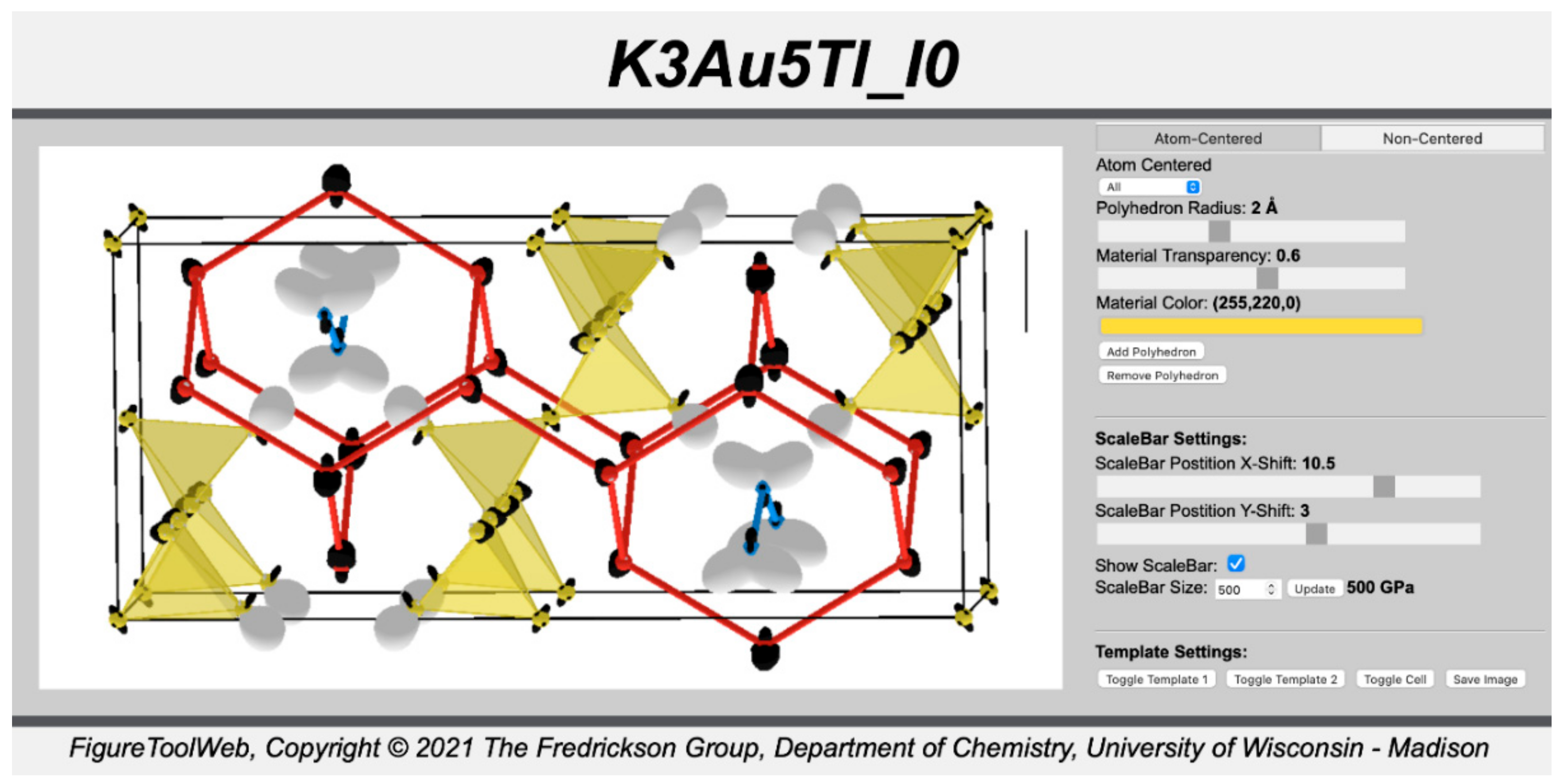
Finally, the sizes of the CP features can be adjusted by changing the CP scale value and pressing the update button. In general, the scale should be set as high as possible without allowing the CP lobes on neighboring atoms to completely obscure the spaces between the interacting atoms. To enable quantitative comparisons of the CP features between structures, a scale bar can be added using the toggle button under the Scalebar Settings and adjusted using corresponding slider elements (Figure 10). Here, the scale bar is chosen to represent 500 GPa and set at the top right of the window. Once we are satisfied with the image, we can capture the contents of the window using the Save Image button.

9. Interpretation of the CP Schemes

Over the course of Section 3, Section 4, Section 5, Section 6, Section 7 and Section 8, we have gone from K₃Au₅Tl’s CIF file to 3D renderings of its CP scheme. Let’s now see how the scheme can be examined to answer questions about the atomic packing issues that have shaped this structure. Our choice of this compound as a demonstration system was motivated by its relationship to two parent structures (Figure 1), the hypothetical phases MgCu₂-type KAu₂ and NaTl-type KTl (both of which represent plausible alternatives to the experimentally observed structures of these compounds)³. To facilitate this analysis, then, we repeat the above steps for KTl in NaTl type and KAu₂ in MgCu₂ type to generate their CP schemes for comparison with K₃Au₅Tl, as shown in Figure 11 [74].

To help detect trends in the CP features among these structures, we start by reviewing their structural parallels and differences (Figure 1). The most prominent commonality is the presence of a cubic diamond network of K atoms in all three structures whose adamantane-like cages serve as hosts for the atoms of the other elements. Each of these adamantane-like cages corresponds to one K atom per formula unit, with the remaining atoms in the formulas corresponding to the contents of the cages. In KAu₂, the “Au₂” of the formula unit corresponds to one Au₄ tetrahedron in each cage with all of its vertices shared with one other tetrahedron, i.e., KAu₂ = KAu_4/2. In KTl, the Tl₁ in the formula corresponds to one Tl atom in each cage.

The formula for K₃Au₅Tl can be derived in a similar fashion. Two thirds of the K adamantane cages are occupied by Au₄ units, while one third of them are filled by single Tl atoms. As the Au₄ units are this time only sharing three of their four corners, each now contributes Au_{3/2 + 1} = Au_{4/2 + 1/2} to the structure. The Tl atoms, on the other hand, are linked together into zigzag chains, remnants of the Tl diamond network present in the full KTl structure. Overall, then, the intergrowth character of the phase is captured by expressing its formula as K₃Au₅Tl = 2(KAu₂ + ½Au) + KTl.

The K diamond networks in the structures also form a useful starting point for a comparison of the CP schemes (Figure 11). In KTl in NaTl type, there are exclusively positive CPs between K atoms on the diamond network, which is represented by white lobes pointing along the shortest K-K contacts. The desire for expansion of the K diamond network here is hindered by negative CPs between the Tl atoms, indicating that the contacts with the Tl diamond are overly extended. Indeed, the stability of the observed structure of KTl over this NaTl-type has been attributed to the inability of the Tl atoms to approach each other closely enough to make sufficiently strong and directional Tl-Tl bonds [74].

For KAu₂ in the MgCu₂ type, the situation is nearly reversed. There are exclusively negative CP features that surround the K atoms on the diamond network, revealing that the K-K and K-Au distances are longer than would be ideal in this electronic context. Contraction of the structure to satisfy the preferences for shorter distances, however, is counteracted by the positive CP along the Au-Au contacts in Au sublattice.

These two CP schemes set up a fascinating complementarity between adamantane cages occupied by Au₄ tetrahedra and Tl single atoms. In the former, the K atoms are under-coordinated, seeking stronger interactions from all directions, while in the latter the coordination environments are over-crowded. Placing Tl-atoms and Au₄ tetrahedra in neighboring adamantane cages could provide a means to tune the packing of the K atoms shared by the cages. In addition, an opportunity for CP relief could occur at the point where the Au₄ tetrahedron in one cage approaches the Tl atom in another. Here, the corner Au atom that would experience positive pressure from the neighboring cage in KAu₂ now approaches a Tl atom that would experience negative pressure from the opposite direction in KTl. The potential release of these forces at the interface between the cages would then open paths for relief of CP elsewhere.

A look at the CP scheme of K₃Au₅Tl indeed reveals significantly smaller CP features throughout most of the structure compared to their counterparts in the binary structures, especially relative to KAu₂. For instance, although the two distinct K sites in K₃Au₅Tl bear very different negative CPs, the site with larger CP lobes has smaller or comparable pressures compared to those of K atoms in the diamond network in either binary structure, while the other site has even smaller pressure features. The Au-Au positive CPs have also become significantly reduced relative to those in KAu₂.

The main exception to the general relief of the CPs relative to the parent structures is at the new Tl-Au contacts. In fact, the positive CP that emerges here is now perhaps the most prominent feature in the CP scheme. While this new interaction may seem like it detracts from the favorability of structure (though the binary structures offer little basis for comparison, as they have no Tl-Au interactions), it also sets up an important synergy in the displacements of the atoms away from their ideal locations in the original KAu₂ and KTl structures. Whereas in these parent structures the Au₄ tetrahedra and Tl atoms were exactly at the centers of the adamantane cages, these positive Tl-Au pressures break this symmetry. The Tl atoms are displaced away from the interface with the K-Au domains toward their remaining Tl neighbors, which were too distant in the KTl parent structure. This Tl-Au positive pressure also induces a twisting of the networks of Au₄ tetrahedra (corresponding to a soft phonon mode correlated with quadrupolar CP features in the Laves phases we previously investigated) [22,23,25]. This motion pushes the Au atoms away from the Tl-rich regions of the structure and toward K atoms with fewer short contacts to the Tl. The stronger K-Au interactions lead to more of the positive features in the CP map associated with the core-regions of the Au atoms being assigned to these interactions rather than the Au-Au ones, leading to more equalized pressures.

In summary, the favorability of an intergrowth between NaTl-type KTl and MgCu₂-type KAu₂ to form K₃Au₅Tl can be anticipated from the CP features of their parent structures. The K atoms in the two structures appear to have atomic packing densities that are non-ideal in opposite directions, leading to the possibility of a cancellation of strain at an interface. At the same time, the positive CPs on the corners of the Au₄ tetrahedra in MgCu₂-type KAu₂ and negative CPs on the Tl atoms in NaTl-type KTl seem prepared to fit together in a lock-and-key fashion at such an interface. The CP results for the ternary structure affirm these basic expectations, but also highlight how atomic relaxations driven by the geometry at the interface serve to simultaneously enhance the Tl-Au, K-Au, Tl-Tl, and Au-Au interactions. Remarkably, the effectiveness of such stabilization mechanisms is able to overcome a substantial mismatch in the cell parameters for the two parent structures, with a = 7.84 Å and 6.89 Å in the LDA-DFT optimized structures of MgCu₂-type KAu₂ and NaTl-type KTl, respectively.

10. Conclusions

In this article, we have provided a step-by-step guide to the creation and interpretation of the CP schemes of solid-state structures, with the packing contributions to the stability of K₃Au₅Tl over its binary parent structures serving as a worked example. Overall, there are four steps to this process: (1) the DFT calculations for generating the necessary electronic structure information, (2) the partition of the contributions of the E_α + E_Ewald and E_nonlocal components of the total energy, (3) the calculation of atomic charges and the generation of corresponding free-ion electron densities for the Hirshfeld-inspired contact volume construction, and (4) the creation and interpretation of the CP schemes. For each of these steps, we have introduced new programs that streamline the workflow. The full CPpackage, apeDEN_files, and associated FigureToolWeb utility are freely available at the DFT-CP GitHub page, URL: https://www.GitHub.com/Fredrickson-UW/DFT-CP/, accessed on 26 July 2021.

In terms of our analysis of K₃Au₅Tl, we found that its formation can be rationalized as a CP-driven intergrowth between hypothetical NaTl-type and MgCu₂-type polymorphs of KTl and KAu₂, respectively. The two parent structures exhibit complementary CP features that anticipate the favorability of their intergrowth. These include the opposite signs of the CPs on the atoms of the K sublattices, which in both cases adopt a diamond network, as well as the potential docking of positive CPs on the corners of the Au₄ tetrahedra in KAu₂ with negative CPs on the Tl atoms of KTl at interfaces between the two structures. In the actual intergrowth structure, the CP relief provided by these interfaces is supported by structural relaxation, which features the twisting of the network of vertex-sharing Au tetrahedra, the contraction of the remaining Tl-Tl contacts, and the stronger interactions at some of the K-Au contacts. The detailed matching of the atomic positions and complementary CPs at the KAu₂/KTl interface illustrates the more general phenomenon of epitaxial stabilization in intermetallic intergrowth structures [35,37,38,39].