Article

Real Time Predictions of VGF-GaAs Growth Dynamics by LSTM Neural Networks

1
Leibniz-Institut für Kristallzüchtung, Max Born St. 2, 12489 Berlin, Germany
2
Institute of Control Theory, TU Dresden, Georg Schumann St. 7a, 01187 Dresden, Germany
3
Leibniz Institute for Catalysis, Albert Einstein St. 29A, 18069 Rostock, Germany
4
Institute of Computer Science, Pod Vodárenskou Věží 2, 18207 Prague, Czech Republic
*
Author to whom correspondence should be addressed.
Crystals 2021, 11(2), 138; https://doi.org/10.3390/cryst11020138
Submission received: 28 December 2020 / Revised: 22 January 2021 / Accepted: 25 January 2021 / Published: 29 January 2021
(This article belongs to the Special Issue Artificial Intelligence for Crystal Growth and Characterization)

Abstract

:
The aim of this study was to assess the aptitude of the recurrent Long Short-Term Memory (LSTM) neural networks for fast and accurate predictions of process dynamics in vertical-gradient-freeze growth of gallium arsenide crystals (VGF-GaAs) using datasets generated by numerical transient simulations. Real time predictions of the temperatures and solid–liquid interface position in GaAs are crucial for control applications and for process visualization, i.e., for generation of digital twins. In the reported study, an LSTM network was trained on 1950 datasets with 2 external inputs and 6 outputs. Based on network performance criteria and training results, LSTMs showed the very accurate predictions of the VGF-GaAs growth process with median root-mean-square-error (RMSE) values of 2 × 10⁻³. This deep learning method achieved a superior predictive accuracy and timeliness compared with more traditional Nonlinear AutoRegressive eXogenous (NARX) recurrent networks.

1. Introduction

GaAs is one of the crucial future materials for microelectronic and optoelectronic devices in 5G and 6G technologies [1] that provides access to terahertz frequencies and real-time transmission for the next generation of wireless communications. The maturity level of 5G and 6G technologies highly depends on the advancement in Vertical-Gradient-Freeze (VGF) method of GaAs manufacturing. Devices are sensitive to GaAs crystal defects that induce leakage currents, which can dramatically deteriorate device performance. Since density and electrical activity of defects is influenced by the thermal history of the GaAs crystal, in operando process monitoring, earlier fault detection and precise control of crystal growth process are essential.
More precisely, a time variant spatially distributed temperature profile inside the GaAs has to be established and tracked while only using limited spatially lumped controls on the outside. This boundary control problem is made even more difficult, because the resulting partial differential equations for the temperature distribution in crystal and melt are coupled by the dynamics of the crystallization front and thus form a nonlinear free boundary problem.
Moreover, direct measurement of temperature, velocity and concentration fields in the melt and crystal may cause contamination and is, therefore, troublesome. Predictions for the transport phenomena during crystal growth based on computational fluid dynamics (CFD) numerical modeling are accurate, but too slow for real time applications like Model Predictive Control. When applying such a control scheme, several complete simulations of the whole process must be computed to find the optimal control input every time a new input is needed. This typically requires solving times of about 1 min for a 76 h process.
Difficulties lie i.a. in the fact that a VGF-GaAs growth process is transient in nature with duration up to 3 days and pronounced time lag effect. The later originates from low heat conductivity of GaAs (λm = 0.178 W/cm/K and λs = 0.071 W/cm/K at Tm = 1512 K) that hampers latent heat removal. The growth rate is slow (~2–4 mm/h), process temperature range narrow (grad Tmelt ~ 2–5 K/cm; grad Tcrystal ~ 15 K/cm) and critical shear stress low (σcr = 0.587 MPa at 40 K below Tm) [2].
One feasible solution for the generation of digital twins and process control is the application of machine learning (ML) and particularly artificial neural networks (ANN) for the fast forecasting of the VGF-GaAs growth process. Application of ML to crystal growth is a new, but fast emerging and very promising field, as shown in, e.g., [3,4,5,6,7,8,9,10,11,12].
Recurrent neural networks (RNN) are a class of ANNs used in cases where the data to be learned are sequential, as it is the case with time series. For them, an RNN response at any given time depends not only on the current input, but on the previous input sequence. Consequently, RNNs have a memory and can be trained to learn transient patterns. RNNs come in many variants [13]. In our previous proof-of-concept study [3], we used the Nonlinear AutoRegressive eXogenous (NARX) [14] type of RNNs for the prediction of temperature profiles and the s/l interface position in VGF-GaAs growth. The predictions were accurate for slow growth rates, but their accuracy significantly decreased with the increase in the crystal growth rate. In our follow-up study, we increased the number of training datasets from 500 to 2000, but no improvement in prediction accuracy was observed. The reason may lie in the combination of the pronounced time lag effect of GaAs growth and NARX known difficulties in learning long-term dependencies due to their vanishing gradient problem, pertaining to gradient learning methods, such as backpropagation. In such methods, each of the neural network’s weights receives an update proportional to the current gradient of the error function in each iteration of the training process. If the gradient is too small, the weights will not change and the neural network training stops or shows no improvement.
A solution to the vanishing gradient problem could be the application of Long Short-Term Memory (LSTM) networks that were specially developed to deal with both, the short and long-term dependencies [15]. A first successful application of LSTM networks in crystal growth was described in [5] for the process control of Cz-Si growth. The authors used experimental data, i.e., time series of a heating power (1 input) and crystal diameter (1 output) to train an LSTM neural network and derived an LSTM-based identification model. The pulling rate was varying along a given curve and was not used as an input. The concept of identification is demonstrated by showing that the unknown parameters in the studied model are only functions of identified parameters and that these functions lead to unique solutions [16].
In this study, we will present the first results of the application of LSTM networks in the fast prediction of VGF-GaAs crystal growth trained on 1D CFD datasets with temporal profiles of heating power (2 inputs) and temperatures at different positions in GaAs as well as the position of the crystallization front (6 outputs). The final goal is to set up mathematical models of the crystal growth process that are sufficiently precise, real-time capable and structurally suitable both for control applications and for generation of digital twins. Pros and cons of this approach will be discussed and results compared with previous NARX predictions.

2. Models and Methodology

2.1. Generation of Training Data

Transient datasets were generated by numerically solving a 1D model of VGF-GaAs growth as described by Equations (1)–(5) below with initial and boundary conditions given in Equations (4)–(6). The GaAs material properties were taken from [17,18]. A simplified schema of the VGF-GaAs model is shown in Figure 1. While the initial conditions always corresponded to a crucible containing fully molten GaAs with a certain axial temperature gradient, different growth velocities were chosen for which the resulting trajectories of the temperature profile and heater powers by means of a flatness-based feedforward design [19,20]. The same approach was used for data generation in our previous paper [3]. However, this time we extended the total number of datasets from 500 to 1950, each with 100 time steps.
Please note that there is no generic way to determine a priori the required volume of training data, given just a problem description. The number of datasets for training a neural network has to be at least as high as the number of network parameters in order to provide the identifiability of all parameters. However, a sufficient data volume can be diagnosed only by monitoring the performance of the neural network during training.
In our study, one dataset included 2 inputs and 6 outputs denoted as x1, x2 and y1–y6, respectively. The inputs were temporal incoming and outgoing heat fluxes q0 and q1. The outputs included temporal temperature profiles in in GaAs at 0–25–50–75–100% of its total length L and GaAs s/l interface position (corresponding to the crystal length). GaAs growth rates varied in the range of 1 to 5 mm/h. The maximal crystal length was L = 0.3 m. Total crystal growth time was 2.1 × 10⁵ s (58.3 h).
The numerical model was solved using the differential Equation stated in [19,20]:
t T ( z , t ) = α 2 z 2 T ( z , t )
T ( z S , L ( t ) , t ) = T m
  Δ H S , L   t   z S , L ( t ) = λ S z   T ( z S , L ( t ) , t ) λ L z   T ( z S , L + ( t ) , t )
λ L z T ( L , t ) = q 1 ( t )
λ S z T ( 0 , t ) = q 0 ( t )
T ( 0 , 0 ) = T m
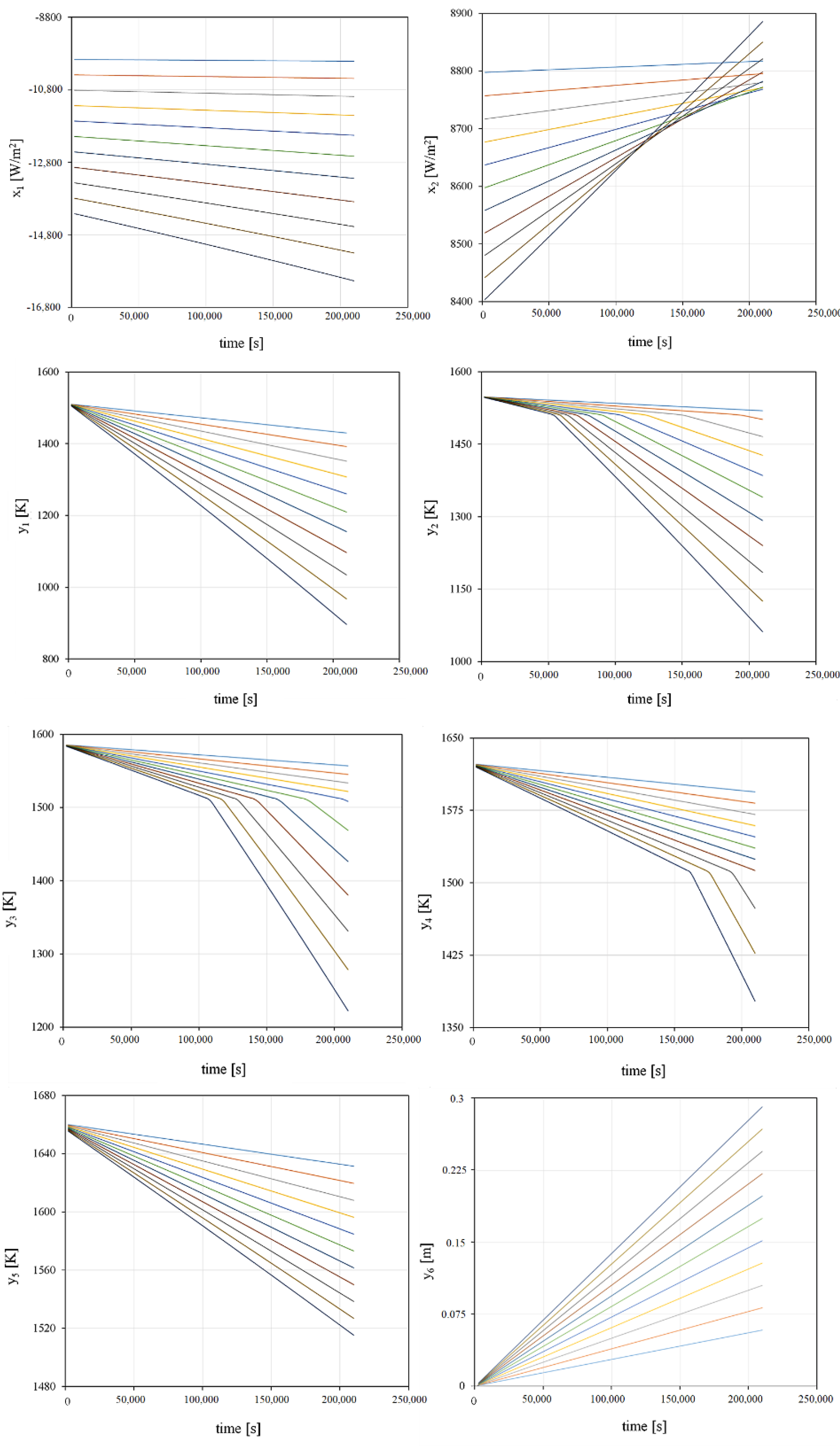
Selected examples of generated training data that served as the temporal input and output datasets for LSTM network are presented in Figure 2.

2.2. LSTM Neural Network Modeling

In contrast to widely used feed forward neural networks where information moves only in forward direction from the input nodes organized in the input layer, through the hidden nodes in hidden layers to the output nodes in the output layer, RNNs are a type of neural networks that are characterized by connections between neurons in one layer and neurons in the same, or a previous, layer, i.e., where the inputs are not independent. RNNs response at any given time depends not only on the current input, but also on the history of the input sequence, RNNs behave like they have a memory. RNNs are typically used in cases where the data to be learned are sequential, i.e., for problems dealing with trajectories, control systems, robotics, speech recognition, language translation, stock predictions, etc.
Despite the fact that basic RNNs are a very powerful method for prediction of time series, still they include many hyperparameters, which are parameters that are not the result of learning. They are either properties of the network that act as constants from the view of the learning algorithm or they affect the learning algorithm itself. Therefore, they are generally difficult to train and may suffer from the vanishing or exploding gradients problem that hinders them to learn long term dependencies. The LSTM network proposed by Hochreiter and Schmidhuber in 1997 [15] successfully addressed these initial shortcomings and became the most popular RNN type nowadays.
An LSTM architecture (see Figure 3) includes several LSTM layers that consist of blocks which in turn consist of cells. Each cell has its own inputs, outputs, and memory. Cells that belong to the same block, share input, output, and forget gates. Input gate decides whether a given information is worth remembering, forget gate decides how much a given information is still worth remembering, i.e., how quickly it may be forgotten and output gate decides whether a given information is relevant at a given step and should be used. Each of these gates can be thought of as a neuron and LSTM cell as a hidden layer in a feed-forward neural network.
The first LSTM block uses the initial state of the network and the first time step of the sequence to compute the first output and the updated cell state. At time step t, the block uses the current state of the network and the next time step of the sequence to compute the output and the updated cell state, as shown in Equations (7)–(11):
f t = σ g ( W f x t + R f h t 1 + b f )
i t = σ g ( W i x t + R i h t 1 + b i )
o t = σ g ( W o x t + R o h t 1 + b o )
g t = σ c ( W g x t + R g h t 1 + b g )
h t = o t σ c ( c t )
where ⊙ denotes the elementwise product of vectors and matrices, aka Hadamard product.
In the Equations (7)–(11), ht R d is a vector which denotes the hidden state of the cell, where d is the cell dimension. xt R d and ht R d denote input and output of the cell at a time step t, respectively. Ri, Ro, Rf, Rg R d × d denote the weight matrices of the input gate, output gate, forget gate and the cell state, respectively.
Similarly Wi, Wo, Wf, Wg   R d × d and bi, bo, bf, bg R d denote the weight matrices corresponding to the current input and the bias vectors, respectively. The symbols gt, it, ot, ft,   R d are the cell candidate, input, output, and forget gate vectors.
The cell state at time step t is given by:
c t = f t c t 1   + i t g t
with σg denoting an componentwise applied gate activation function, which is, by default, the sigmoid function that outputs values in the range [0, 1]:
σ g ( x ) = ( 1 + e x ) 1
In this study, we focused on an LSTM network with altogether 4 layers: input, LSTM, fully connected, and output layer. In LSTM layer, state and gate activation functions were tanh and sigmoid, respectively.
Training an LSTM network includes selecting an optimizer and the number of delay steps, the target prediction accuracy, as well as other options.
Among many, optimizers encountered in deep learning, which are typically using stochastic gradient descent (SGD), the Adam optimizer [21] was selected for this study, due to its superior performance in terms of convergence speed.
The number of time delays was set to 3.
Data preprocessing included data normalization and classification.
First of all, we normalized the data into the interval [0, 1], separately for the inputs x1 and x2 (heat fluxes), for the outputs y1–y5 (temperatures at monitoring points in GaAs), and for the output y6 (the position of the solid-liquid interface).
We used 10% of the total number of datasets for testing and the remaining ones for training. To this end, we took a random permutation of the numbers between 1 and total number of datasets and assigned its last 10% of elements as indices to the test samples and the first 90% of elements as indices to the training samples. This methodology was selected rather than the information richer cross validation [22] due to its much lower computational demands.
A number of hyperparameters are associated with LSTM network training, which require proper tuning. Some important hyperparameters concerning the learning algorithm include: mini-batch size, number of epochs, epoch size, learning rate, number of hidden layers, and validation frequency. The mini-batch size means the number of data sets considered for each gradient descent step full update of the weights through back-propagation. An epoch denotes one full forward and backward pass through the whole dataset. Consequently, the number of epochs denote the number of such passes across the dataset that are required for the optimal training. The learning rate is the intensity with which gradient descent influences the update. If the learning rate is too low, then training takes a long time. If it is too high, then training might diverge. The initial learning rate for the Adam optimizer was set to 0.001.
The optimal network and learning hyperparameters are different for different kinds of training data, it is related to how diverse the training data is. Moreover, some hyperparameters are interdependent (e.g., batch size may interact with learning rate). In this study, the hyperparameters were tuned manually [23].
Altogether, 21 combinations of three learning hyperparameters and of data volume were considered during the hyperparameter tuning, given in Table 1.
In our study, learning was always performed for the maximum number of epochs.
The accuracy of predictions yp,i relative to actual target yi for each of the 100 time steps in all 1950 datasets was estimated using the root mean squared error (RMSE), defined in Equation (14). Herein, a lower RMSE implies a better prediction accuracy.
R M S E = i = 1 n ( y p , i y i ) 2 n
Due to low critical shear stress of GaAs and the associated high risk for polycrystalline growth, for practical applications and especially for feedback control, a high prediction accuracy is required for the process temperatures. Therefore, in this study, the LSTM prediction accuracy was assessed based on the whole distribution of obtained RMSE values.
For ANN simulations, the commercial software Matlab® and its Neural Network Toolbox™ were used.

3. Results and Discussion

Our goal was to assess the predictive accuracy of LSTM networks using datasets generated by numerical transient simulations of the VGF-GaAs growth process. A performance comparison between the various LSTM networks with combinations of learning-hyperparameters described in Table 1 was carried out and the results shown in Figure 4, Figure 5, Figure 6, Figure 7, Figure 8 and Figure 9 are summarized below.
The identification of suitable LSTM learning-hyperparameters and data volume started with a comparison of RMSE values in cases where one feature was varied while the rest was kept constant. The reference combination 1 corresponds to 1950 datasets, optimizer Adam, initial learning rate 1 × 10⁻³, mini batch size 225, maximum number of epochs 100, and a validation frequency of 50.
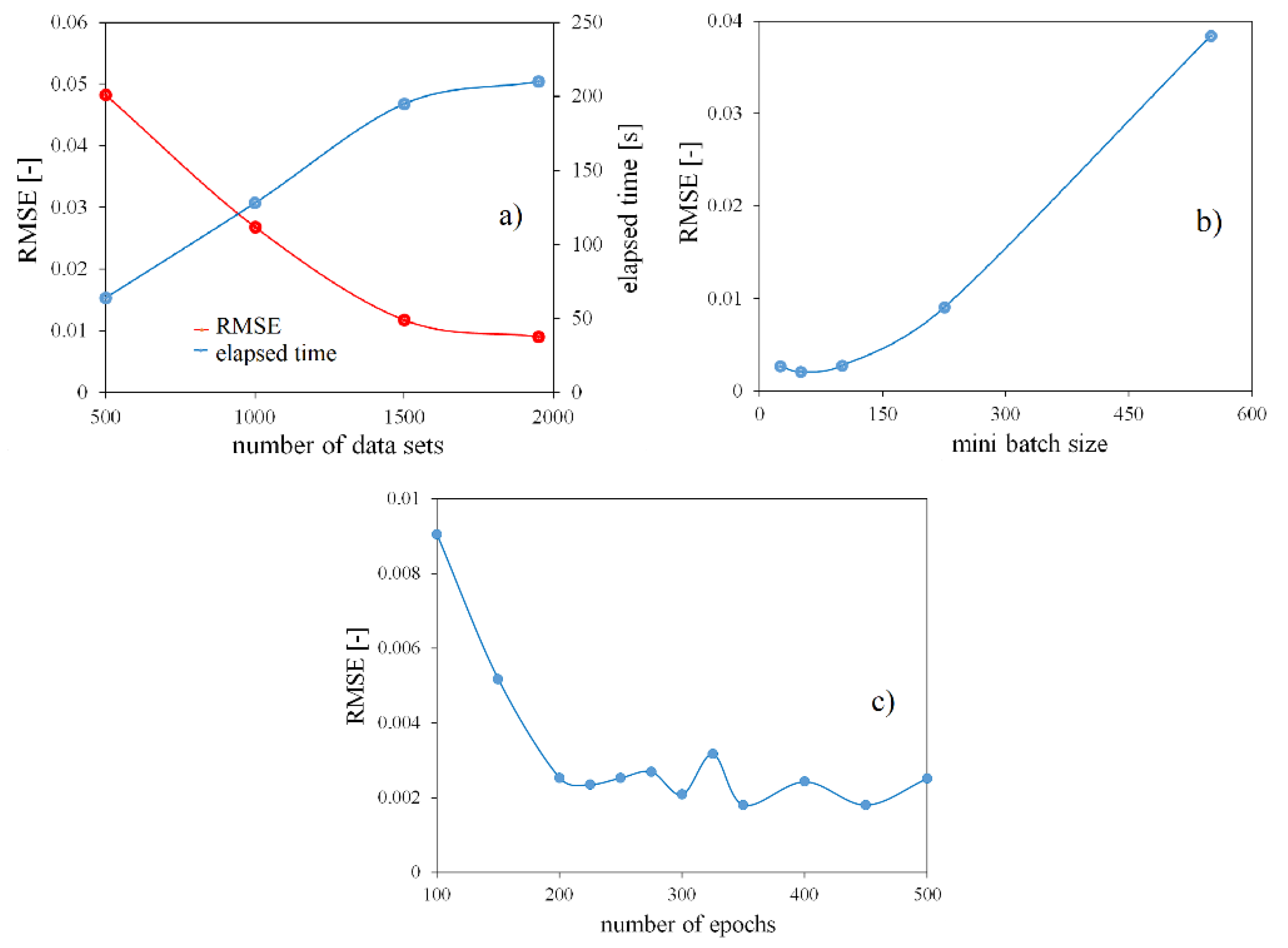
The influence of data volume and elapsed time for network training on the LSTM prediction performance was obtained by comparison of combinations 1–4. Results are shown in Figure 4a. By tripling the data volume from 500 to 1500 datasets, RMSE decreased 5 times from ~5 to ~1%. However, a further increase in the data volume to 1950 datasets only insignificantly improved the RMSE value. Elapsed time showed the reciprocally trend and it was in all cases less than 200 s.
The influence of mini batch size values in the range from 25 to 550 on the RMSE was studied via comparison of combinations 1 and 5–8. The results were shown in Figure 4b. It has been observed that when using a larger batch size of more than 100, there is a degradation in the prediction accuracy in terms of the RMSE. This finding is a consequence of the fact that large-batch methods tend to poorer generalization.
The influence of the number of epochs in the range 100–500 on the RMSE value was obtained by comparison of combinations 1 and 9–19. The results are shown in Figure 4c. A strong decrease in the RMSE value was observed with an increase in the number of epochs from 100 to 200. A further increase in this parameter influenced the RMSE value only a little.
As mentioned before, the predictive power of LSTM in GaAs growth must be assessed using the whole distribution of RMSE values. This approach is obvious if different properties of that distribution are plotted for different datasets and hyperparameters.
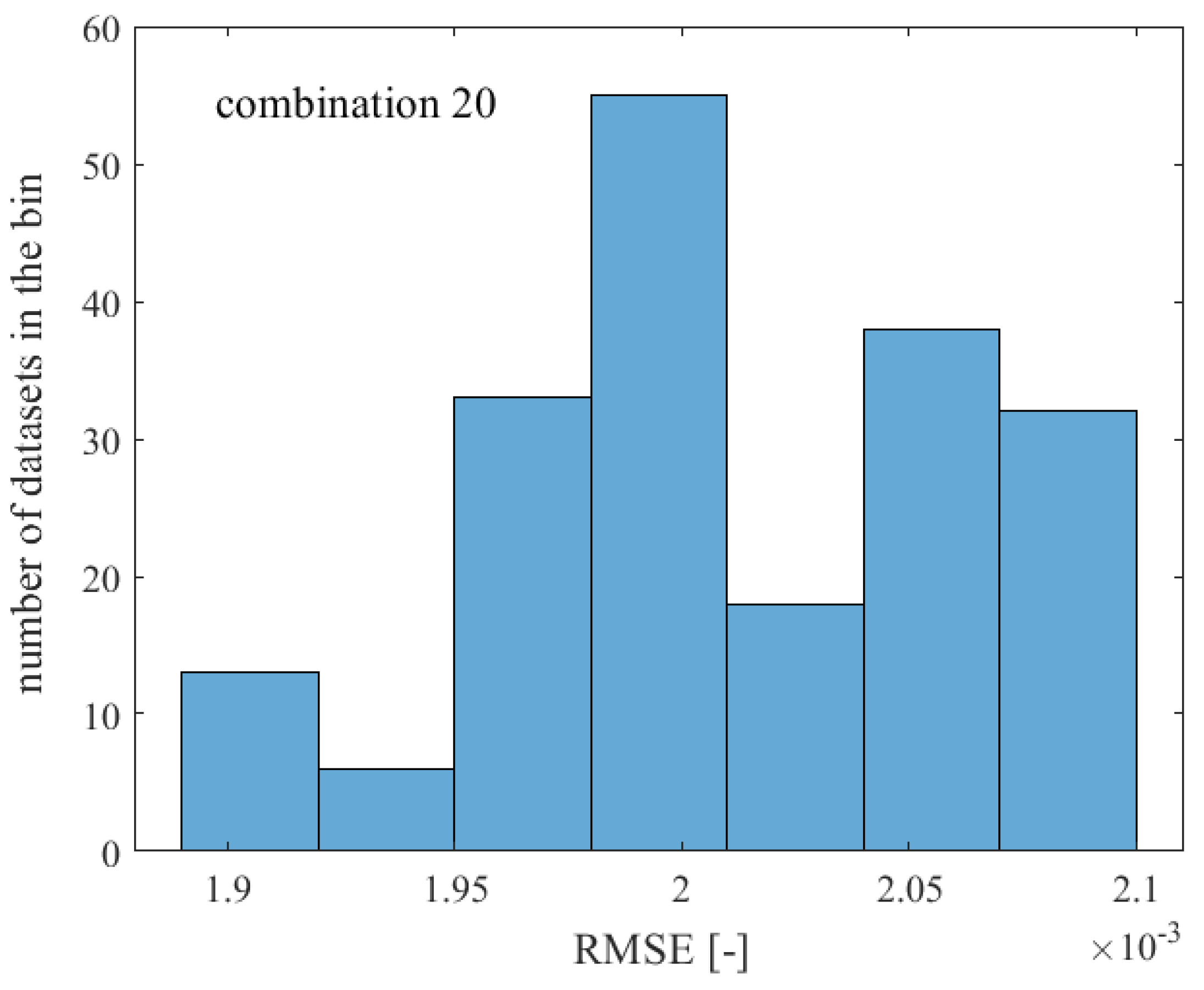
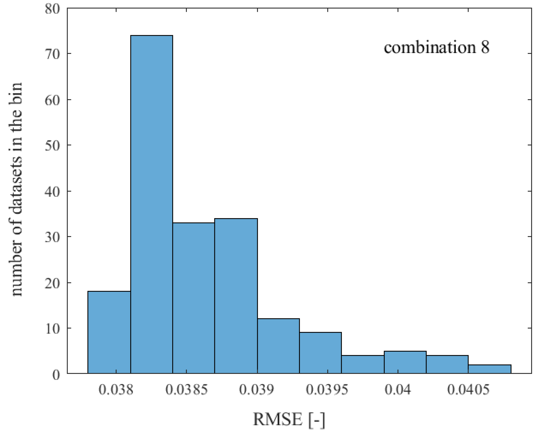
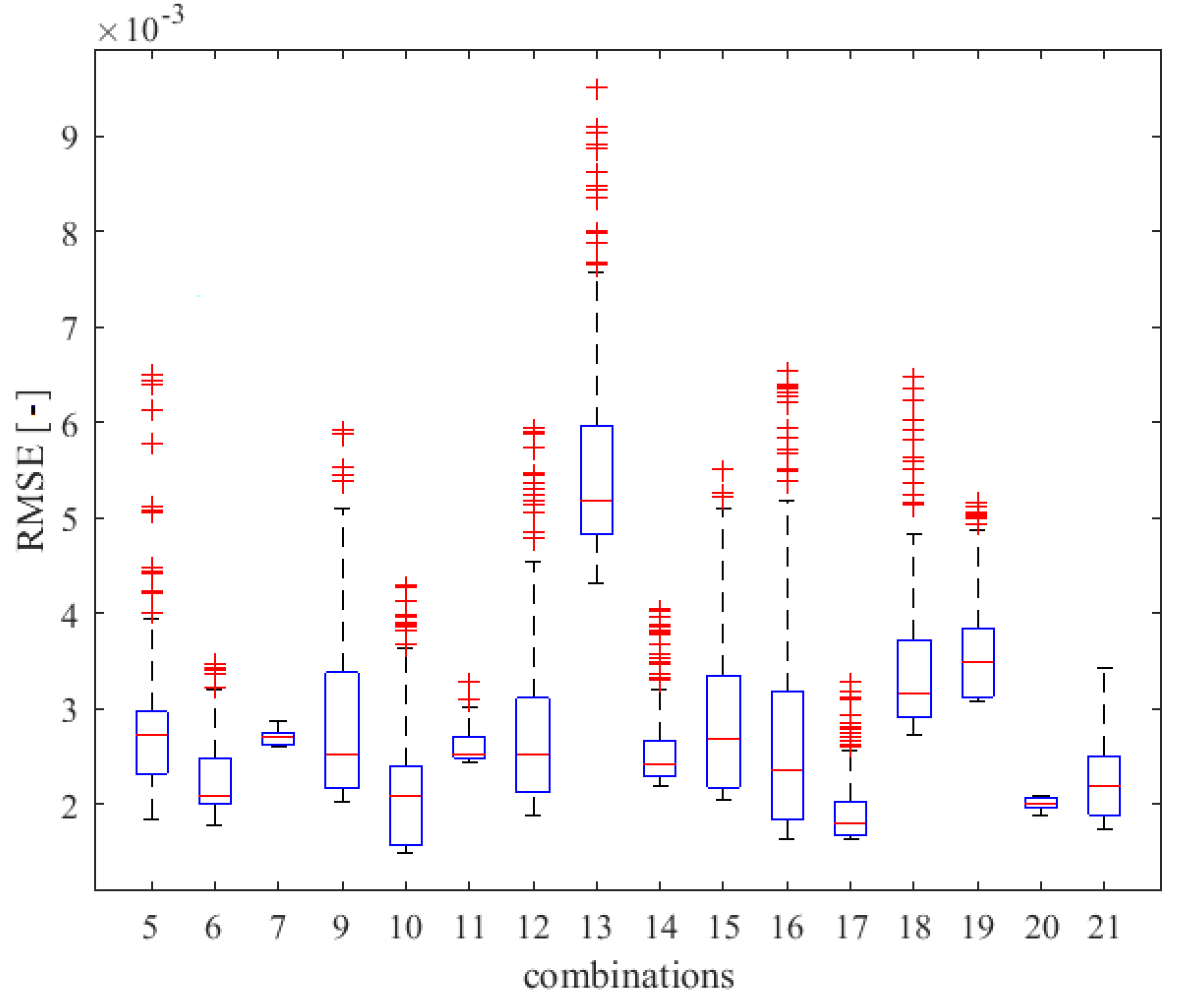
In Figure 5 and Figure 6, RMSE values for the randomly selected datasets for testing are shown, with the learning hyperparameters corresponding to the combinations 20 and 8. The RMSE median value for the combination 20 was one order of magnitude lower than for the combination 8 (2.0076 × 10⁻³ vs. 3.845 × 10⁻²). Similarly, also the variance of RMSE values was lower.
The RMSE box plots for the studied combinations is given in Figure 7. The cases 1–4 and 8 show an order of magnitude higher RMSE values than the rest. The best overall performance was obtained for the combination 20 with one of the lowest median RMSE values (2.0076 × 10⁻³), narrow interquartile range values and no outliers. In LSTM layer, input size and number of hidden units were 20 and 100, respectively.
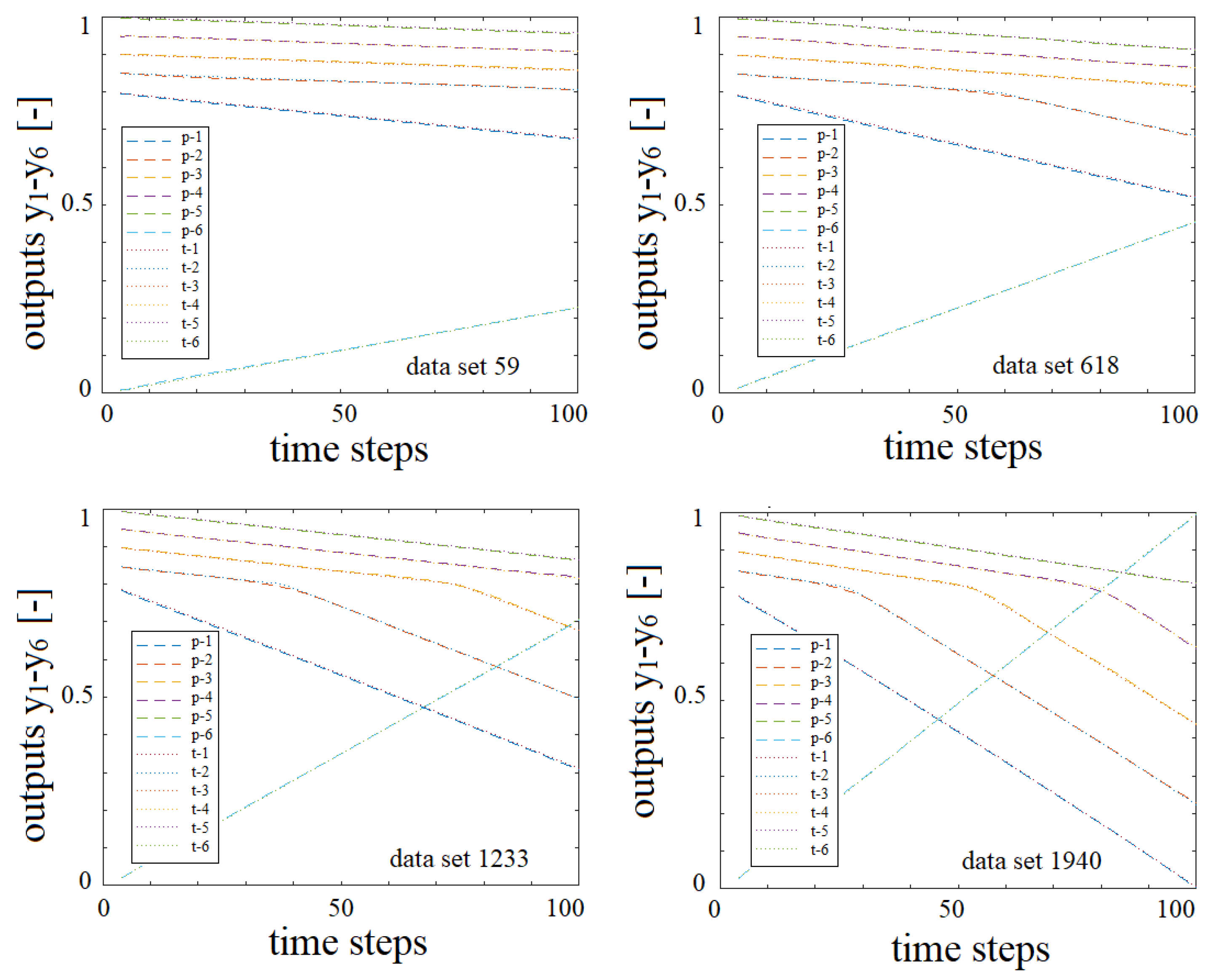
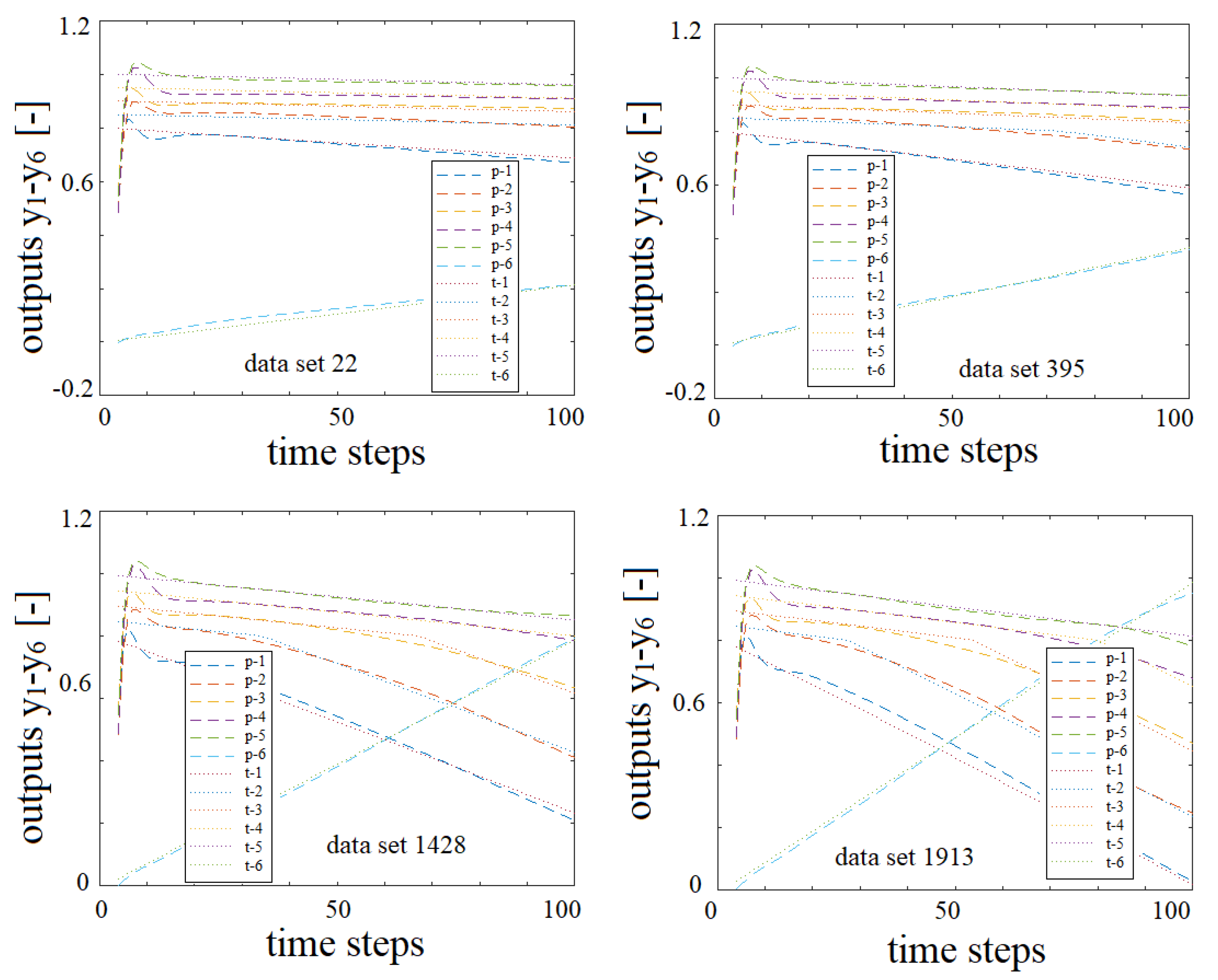
Another way of assessing the quality of network predictions is to compare LSTM predicted versus targeted temporal profiles of output variables y1–y6. For cases 20 and 8 and several selected datasets, results are given in Figure 8 and Figure 9, respectively.
In both figures, the results are shown for four exemplary datasets that are differing in crystal growth rates. For example, among the four datasets in Figure 8 (combination 20), the datasets 59 corresponds to the lowest growth rate, while the dataset 1940 to the highest growth rate. Consequently, the crystal length, i.e., the value of the output y6 in dataset 1940 in the last time step was the highest. For all datasets, the predicted outputs values accurately follow the targeted values.
Similarly, in Figure 9 (combination 8), the grow rate increased from the dataset 22 over 395 and 1428 to 1913. In this case, the predicted outputs differed strongly from the target outputs at the beginning of the growth process, i.e., in the time steps 1–15, for all growth rates. Additionally, predictions were inaccurate at the time steps when crystallization front passed by the location of the monitoring point and temperature profile suddenly changed slope (see also Figure 2).
Summarizing the obtained results, the LSTM network with learning hyper-parameters and data volume according to the combination 20 accurately predicted VGF-GaAs dynamics without difficulties in learning high crystal growth rates that we previously observed when using NARX networks. In addition, no observed outliers in the prediction of outputs decreased the risk for polycrystalline growth in the real process.
Considering the computational burden, i.e., the average training time for the same datasets, LSTM networks again overperformed NARX networks significantly.
For example, in our previous study, training of NARX network on 500 datasets using Bayesian Regularization and Levenberg–Marquardt training algorithm, at a personal computer with Intel Pentium i7-7700K CPU at 4.20 GHz, 64 GB RAM, x64 based processor took 48 and 14 days, respectively. LSTM training on the same 500 datasets took 1 min. at a Windows server with Intel® Xeon® 6234 CPU at 3.30 GHz 3.29 GHz (2 processors), 384 GB RAM, x64 based processor. LSTM training on extended 1950 datasets took up to 19 min. at the same Windows server. Direct comparison of these two studies is not possible due to differences in used hardware. Still, the significantly shorter training time of LSTM network is obvious.

4. Conclusions

This study demonstrated the capabilities of a LSTM neural network in fast forecasting of crystal growth recipes on the example of VGF-GaAs growth. Such real-time predictions are inevitably needed, e.g., in process automation and control.
The accuracy of predictions of growth recipes by LSTM neural networks was superior to NARX predictions.
An accurate and efficient LSTM architecture was identified, determined the hyperparameters and required data volume for the studied parameter space. Based on the statistical performance criteria and training results, the LSTM trained with the Adam optimizer, with 3 time delays, 450 epochs, 50 mini batch size, 1 × 10⁻³ initial learning rate was accurate for our database consisting of 1950 growth recipes generated by 1D CFD modeling. The LSTM accuracy was assessed using the distribution of RMSE values. For the most accurate predictions of VGF-GaAs growth dynamics, the median RMSE value of 2 × 10⁻³ was obtained.
In all cases, the LSTM training was several orders of magnitude faster than NARX training on the same datasets.
Since a LSTM network relies heavily on the availability and the quality of training data, our further efforts have to be directed to generate datasets from transient 2D CFD models.

Author Contributions

Conceptualization, N.D.; methodology, M.H., N.D. and S.E.; software, M.H., N.D. and S.E.; validation, N.D.; formal analysis, N.D., M.H.; investigation, N.D., M.H. and S.E.; writing—original draft preparation, N.D.; writing—review and editing, N.D., S.E. and M.H.; visualization, N.D. All authors have read and agreed to the published version of the manuscript.

Funding

This work was partly funded by the Czech Science Foundation (grant 18-18080S) and the Deutsche Forschungsgemeinschaft (DFG) (project number WI 4412/1-1).

Institutional Review Board Statement

Not applicable.

Informed Consent Statement

Not applicable.

Data Availability Statement

Data is contained within the article.

Acknowledgments

Proof reading of the article by Klaus Böttcher is gratefully acknowledged.

Conflicts of Interest

The authors declare no conflict of interest.

Nomenclature

ΔHS,Llatent heat of solidification [J/m3]
Lcrystal length [m]
Tmmelting temperature [K]
qheat flux [W/m3]
ttime [s]
zaxial coordinate [m]
αthermal diffusivity [m2/s]
λthermal conductivity [W/mK]
ρdensity [kg/m3]

References

  1. Yuan, Y.; Zhao, Y.; Zong, B.; Parolari, S. Potential Key Technologies for 6G Mobile Communications. Sci. China Inf. Sci. 2018, 61, 080404. [Google Scholar]
  2. Frank-Rotsch, C.; Dropka, N.; Rotsch, P. Chapter 6: III-Arsenides. In Single crystals of Electronic Materials: Growth and Properties; Fornari, R., Ed.; Woodhead Publishing Elsevier: Amsterdam, The Netherlands, 2018; pp. 181–240. [Google Scholar] [CrossRef]
  3. Dropka, N.; Holena, M.; Ecklebe, S.; Frank-Rotsch, C.; Winkler, J. Fast forecasting of VGF crystal growth process by dynamic neural networks. J. Cryst. Growth 2019, 521, 9–14. [Google Scholar] [CrossRef]
  4. Dropka, N.; Holena, M. Optimization of magnetically driven directional solidification of silicon using artificial neural networks and Gaussian process models. J. Cryst. Growth 2017, 471, 53–61. [Google Scholar] [CrossRef]
  5. Zhang, J.; Tang, Q.; Liu, D. Research into the LSTM neural network based crystal growth process model identification. IEEE Trans. Semicond. Manuf. 2019, 32, 220–225. [Google Scholar] [CrossRef]
  6. Asadian, M.; Seyedein, S.H.; Aboutalebi, M.R.; Maroosi, A. Optimization of the parameters affecting the shape and position of crystal-melt interface in YAG single crystal growth. J. Cryst. Growth 2009, 311, 342–348. [Google Scholar] [CrossRef]
  7. Tsunooka, Y.; Kokubo, N.; Hatasa, G.; Harada, S.; Tagawa, M.; Ujihara, T. High-speed prediction of computational fluid dynamics simulation in crystal growth. CrystEngComm 2018, 20, 6546–6550. [Google Scholar] [CrossRef] [Green Version]
  8. Tang, Q.; Zhang, J.; Lui, D. Diameter model identification of Cz silicon single crystal growth process. In Proceedings of the 2018 Chinese Automation Congress (CAC), Xi’an, China, 30 November–2 December 2018; pp. 2069–2073. [Google Scholar]
  9. Dang, Y.; Liu, L.; Li, Z. Optimization of the controlling recipe in quasi-single crystalline silicon growth using artificial neural network and genetic algorithm. J. Cryst. Growth 2019, 522, 195–203. [Google Scholar] [CrossRef]
  10. Ujihara, T.; Tsunooka, Y.; Hatasa, G.; Kutsukake, K.; Ishiguro, A.; Murayama, K.; Tagawa, M. The Prediction Model of Crystal Growth Simulation Built by Machine Learning and Its Applications. Vac. Surf. Sci. 2019, 62, 136–140. [Google Scholar] [CrossRef]
  11. Boucetta, A.; Kutsukake, K.; Kojima, T.; Kudo, H.; Matsumoto, T.; Usami, N. Application of artificial neural network to optimize sensor positions for accurate monitoring: An example with thermocouples in a crystal growth furnace. Appl. Phys. Express 2019, 12, 125503. [Google Scholar] [CrossRef]
  12. Qi, X.; Maa, W.; Dang, Y.; Sua, W.; Liu, L. Optimization of the melt/crystal interface shape and oxygen concentration during the Czochralski silicon crystal growth process using an artificial neural network and a genetic algorithm. J. Cryst. Growth 2020, 548, 125828. [Google Scholar] [CrossRef]
  13. Dupond, S. A thorough review on the current advance of neural network structures. Annu. Rev. Control 2019, 14, 200–230. [Google Scholar]
  14. Leontaritis, I.; Billings, S.A. Input-output parametric models for non-linear systems Part I: Deterministic non-linear systems. Int. J. Control 1985, 41, 303–328. [Google Scholar] [CrossRef]
  15. Hochreiter, S.; Schmidhuber, J. Long short-term memory. Neural Comput. 1997, 9, 1735–1780. [Google Scholar] [CrossRef] [PubMed]
  16. Chen, S.; Billings, S.A.; Grant, P.M. Non-linear system identification using neural networks. Int. J. Control 1990, 51, 1191–1214. [Google Scholar] [CrossRef]
  17. Lantzsch, R. VGF Crystal Growth under the Influence of Magnetic Fields. Ph.D. Thesis, TUB Freiberg, Freiberg, Germany, 2009. [Google Scholar]
  18. Willers, B.; Eckert, S.; Nikrityuk, P.A.; Räbinger, D.; Dong, J.; Eckert, K.; Gerberth, G. Efficient melt stirring using pulse sequences of a rotating magnetic field: Part II. Application to solidification of Al-Si alloys. Metall. Mater. Trans. B. 2008, 39, 304–316. [Google Scholar] [CrossRef]
  19. Dunbar, W.B.; Petit, N.; Rouchon, P.; Martin, P. Motion planning for a nonlinear Stefan problem. ESAIM Control Optim. Calc. Var. 2003, 9, 275–296. [Google Scholar] [CrossRef]
  20. Rudolph, J.; Winkler, J.; Woittennek, F. Flatness Based Control of Distributed Parameter Systems: Examples and Computer Exercises from Various Technological Domains; Berichte aus der Steuerungs- und Regelungstechnik, Shaker: Aachen, Germany, 2003. [Google Scholar]
  21. Kingma, D.P.; Ba, J.L. Adam: A Method for stochastic optimization. arXiv 2015, arXiv:1412.6980. [Google Scholar]
  22. Barrow, D.K.; Crone, S.F. Crogging (cross-validation aggregation) for forecasting—A novel algorithm of neural network ensembles on time series subsamples. In Proceedings of the 2013 International Joint Conference on Neural Networks, Dallas, TX, USA, 4–9 August 2013; pp. 1–8. [Google Scholar]
  23. Hutter, F.; Luecke, J.; Schmidt-Thieme, L. Beyond Manual Tuning of Hyperparameters. KI-Kuenstl. Intell. 2015, 29, 329–337. [Google Scholar] [CrossRef]
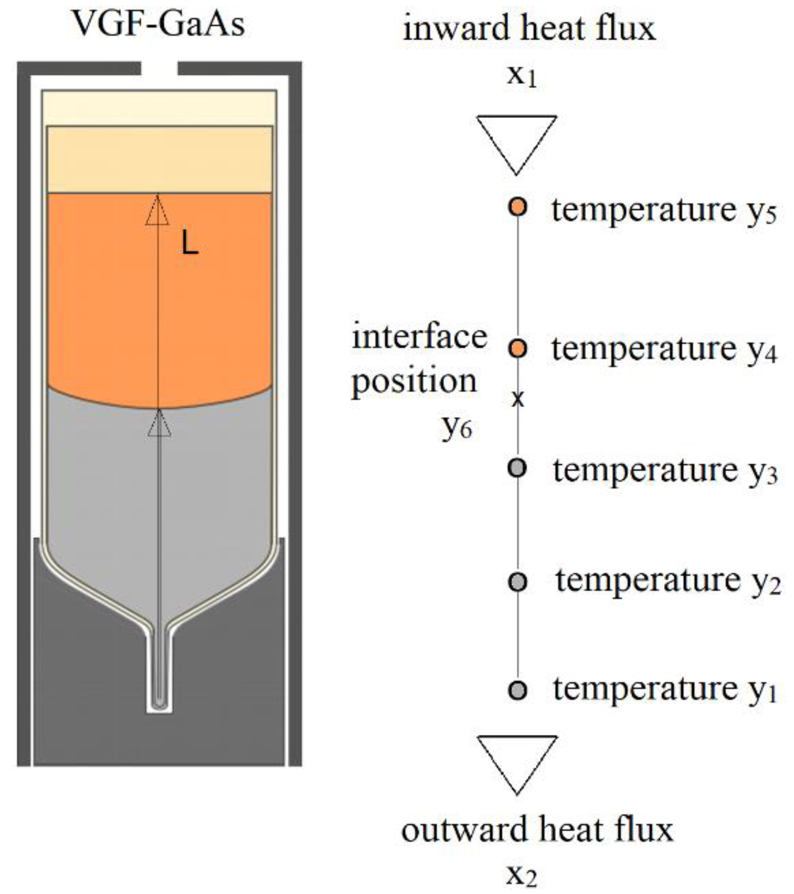
Figure 1. Sketch of the VGF-GaAs hot zone with related neural network inputs (incoming x1 and outgoing x2 heat fluxes) and outputs (temperatures in GaAs at 0–25–50–75–100% of its length y1 to y5 and interface position y6) related to 1D model of melt and crystal.
Crystals 11 00138 g001
Figure 2. Examples of crystal growth datasets: temporal profiles of inputs x1, x2 (incoming and outgoing heat fluxes), temporal profiles of outputs y1 to y5 (temperatures in characteristic points in GaAs) and y6 (interface position in GaAs).
Crystals 11 00138 g002
Figure 3. An LSTM cell with a new cell state ct, hidden states ht, input gate i, output gate o, cell candidate g, and forget gate f at time step t.
Crystals 11 00138 g003
Figure 4. Influence of: (a) data volume (total number of datasets for training and testing); (b) mini batch size; and (c) number of epochs on the RMSE value and in the case of data volume also on the elapsed time of network training. The remaining learning hyperparameters and data volume corresponded to the reference combination: total number of datasets for training and testing 1950, optimizer Adam, initial learning rate 1 × 10⁻³, mini batch size 225, maximal number of epochs 100, validation frequency 50.
Crystals 11 00138 g004
Figure 5. Histogram of RMSEs for random selected 195 datasets for testing using LSTM parameters defined in combination 20. Median RMSE value was equal 2.0076 × 10⁻³.
Crystals 11 00138 g005
Figure 6. Histogram of RMSEs for random selected 195 datasets for testing using LSTM parameters defined in combination 8. Median RMSE value was equal 3.845 × 10⁻².
Crystals 11 00138 g006
Figure 7. RMSE for predictions of datasets for testing, for 17 out of 21 combinations of hyperparameters. For the remaining combinations 1–4 and 8, an order of magnitude higher RMSE values (median values in the range 0.009–0.05) were obtained. The RMSE box plot displays the median (red line), the first and third quartiles, outliers (red ‘+’ symbol), and the range values that are not outliers.
Crystals 11 00138 g007
Figure 8. Comparison of normalized LSTM-predicted outputs (p-1 to p-6) and normalized test outputs (t-1 to t-6) for 4 randomly selected datasets out of the 195 datasets for testing. The learning hyperparameters are given by the combination 20.
Crystals 11 00138 g008
Figure 9. Comparison of normalized LSTM-predicted outputs (p-1 to p-6) and normalized test outputs (t-1 to t-6) for 4 randomly selected data sets out of the 195 datasets for testing. The learning hyperparameters and data volume are given by the combination 8.
Crystals 11 00138 g009
Table 1. Considered combinations of the LSTM hyperparameters and number of data. With all of them, the Adam optimizer, initial learning rate 1 × 10⁻³ were used.
Hyperparameter CombinationNo. of DataMax. EpochsMini BatchValidation Frequency
1195010022550
250010022550
3100010022550
4150010022550
5195010010050
619501005050
719501002550
8195010055050
9195020022550
10195030022550
11195050022550
12195025022550
13195015022550
14195040022550
15195027522550
16195022522550
17195035022550
18195032522550
19195045022550
2019504505050
211950450225100
Publisher’s Note: MDPI stays neutral with regard to jurisdictional claims in published maps and institutional affiliations.