Flow Map for Hydrodynamics and Suspension Behavior in a Continuous Archimedes Tube Crystallizer

Abstract

The Archimedes Tube Crystallizer (ATC) is a small-scale coiled tubular crystallizer operated with air-segmented flow. As individual liquid segments are moved through the apparatus by rotation, the ATC operates as a pump. Thus, the ATC overcomes pressure drop limitations of other continuous crystallizers, allowing for longer residence times and crystal growth phases. Understanding continuous crystallizer phenomena is the basis for a well-designed crystallization process, especially for small-scale applications in the pharmaceutical and fine chemical industry. Hydrodynamics and suspension behavior, for example, affect agglomeration, breakage, attrition, and ultimately crystallizer blockage. In practice, however, it is time-consuming to investigate these phenomena experimentally for each new material system. In this contribution, a flow map is developed in five steps through a combination of experiments, CFD simulations, and dimensionless numbers. Accordingly, operating parameters can be specified depending on ATC design and material system used, where suspension behavior is suitable for high-quality crystalline products.

1. Introduction

Continuous crystallization is a promising operation mode for the small-scale production ($\dot{V}\le 100\mathrm{mL}{\min }^{-1}$) of active pharmaceutical ingredients (APIs) and fine chemicals [1,2,3,4]. Reaching the steady state in continuous operation is advantageous regarding the consistency of product quality, e.g., particle size and its distribution. In addition, higher space-time yield than in batch operation is possible because smaller equipment sizes are required [2,4]. In order to utilize these advantages, however, the steady state must first be reached and then maintained [3]. Here, encrustation and blockage of the continuous crystallizers still remain a major challenge [5].

Existing continuous crystallizer concepts can be classified regarding achievable residence time and width of residence time distribution (RTD) [6]. For process design, a narrow RTD of liquid and solid phase is preferable [7], as the position of liquid and solid elements is predetermined. If the RTD of a continuous downstream process is broad, tracing out-of-specification material is difficult [7]. Through a narrow RTD in combination with flexible residence times, defined product particle sizes with narrow particle size distribution (PSD) can be reached. In this context, we introduced the Archimedes Tube Crystallizer (ATC) as a promising apparatus concept [6]. The apparatus consists of a coiled tube that rotates around its horizontal axis. Segmented flow is achieved by a specifically designed inlet tank that is mounted on the horizontal axis and rotates with the same velocity as the coiled tube. With each rotation, the individual liquid segments are moved through the coiled tube. As a consequence of this design, the apparatus itself works as a pump. Therefore, the usual limitations of residence time in tubular crystallizers due to pressure loss do not apply. In addition, the segmented-flow concept leads to narrow liquid- and solid-phase RTDs which was demonstrated for a prototype with volumetric flow rates from 3–15 mL min⁻¹ and residence times from 4–11 min [6].

The next step towards successful particle engineering entails the understanding of hydrodynamics and suspension behavior. These phenomena are decisive in crystallization regarding agglomeration, breakage, attrition, and blockage of the employed crystallizer. In industry, API process development is carried out within set time frames and under material constraints [1]. To reduce effort in this important time period, apparatus development must provide detailed information about mixing. Then, the only remaining time-consuming step is the adaptation to a specific material system.

Hydrodynamics in coiled structures are dominated by secondary flow patterns caused by centrifugal instabilities [8]. Centrifugal and shear forces move the inner fluid in the tube outward and the outer fluid inward. The resulting so-called Dean vortices enhance radial mixing by overlapping the parabolic laminar flow profile. In single-phase flow, the intensity of secondary flow patterns in coiled structures is characterized by Dean number $Dn$ that is calculated based on Reynolds number $Re$ for inner tube diameter $d_{i,tube}$ and coiled tube diameter $d_{ct}$ as $Dn=Re·\sqrt{d_{i,tube}/d_{ct}}$ [8,9]. Thereby, the coiled flow inverter (CFI) represents an improved helically coiled device design with additional bends between the helical segments. Due to the additional bends, the direction of the centrifugal force is changed at each bend so that the existing flow profile is disrupted and reformed with positive impact on mixing [10].

Air-segmented flow consists, as the name suggests, of a segmented flow of two immiscible fluids, specifically air (or another immiscible gas) and the process medium. For slug formation, usually a mixing piece (e.g., T-junction) is installed to connect process medium and air supply delivered by individual peristaltic pumps [11]. The flow regime in one individual slug is characterized by internal circulations, the so-called Taylor vortices [12]. Due to the enhanced flow regime, air-segmented flow hydrodynamics have mostly been researched as process intensification technique for micro-reactors focusing on heat and mass transfer enhancement [12,13]. Here, Talimi et al. reviewed prior numerical studies of hydrodynamics (computational fluid dynamics (CFD)) and outlined the main factors on flow pattern as bubble length, capillary number Ca, channel curvature (for curved microchannels), and superficial velocities of the two phases, among others [12]. Gaddem et al. investigated segmented flow in coiled structures, specifically in a CFI [14]. For this purpose, they developed a CFD model for the superposition of Taylor and Dean flow to assess the potential improvement in mass transfer for application as a microscale reactor [14]. To describe the effect of flow superposition, the modified Dean number $D{n}^{\ast }$ was introduced [14].

There are also various studies that describe suspension behavior of particles in the previously introduced coiled structures and in segmented flow. Tiwari et al. conducted CFD simulations in a helically coiled device with particles of 1 and 3 μm diameter and volume fraction 0.1 [8]. In the simulations, a deviation in the particle settling zone from tube bottom to inner bend was observed, which was attributed to increased wall shear stress [8]. Dbouk and Habchi observed hydrodynamics and suspension behavior in helical pipes for application as static mixer [15]. The investigated particles were monodisperse (particle size 25–400 μm, initial volume fraction 0.25–0.45), spherical, and had the same density as the Newtonian liquid phase [15]. Under these conditions, better mixing was observed for increasing particle diameter [15]. Wiedmeyer et al. found a size-dependent residence time of potash alum crystals in a helically coiled tube crystallizer, that was attributed to time-dependent secondary flow patterns identified through direct numerical flow simulations [16]. Emerged in the secondary flow, smaller particles take longer flow paths and thus remain longer in the device than larger particles [16]. For a continuous CFI crystallizer with bend angle 90°, Hohmann et al. investigated the suspension behavior for three test systems with solid-phase mass fractions between 0.01 and 0.10$g_S{g}_{Susp}^{-1}$ and particle size fractions up to 180–250 μm [17]. For the selected material systems, they classified the flow into three regimes: stagnant sediment, moving sediment flow, and homogeneous suspension flow [17]. Based on Reynolds number $Re$ and densimetric Froude number $Fr$, a flow map was set up for the investigated operating points that were almost completely allocated to moving sediment flow [17].

For air-segmented or slug flow crystallizers, various studies deal with the qualitative and quantitative evaluation of crystal suspension homogeneity. In general, two research groups found that suspension homogeneity is increased at slug aspect ratios $l_{slug}/d_{i,tube}$ near 1 which also leads to smaller product crystals [18,19]. Jiang et al. used an imaging method based on a stereomicroscope and a video camera for suspension quality evaluation [18]. Later, they refined this method as a real-time imaging method [20]. Due to the microscope placed in top view, however, the influence of gravity on the growing crystals was not taken into account. Su and Gao implemented a CFD simulation to evaluate suspension state and flow trajectory of $\alpha$-glycine crystals (seed main particle size 8 μm, solid mass fraction 1–3$\mathrm{wt}.\%$) [19]. According to the simulations, the highest crystal flow velocities were found at high aspect ratios of 2 [19]. However, crystals are prone to sedimentation at this operating point, so that an aspect ratio of 1 remains the best compromise [19]. In addition, variation of flow rate did not change the suspension state of the crystals [19]. With the small size of the particles investigated, this result was expected. Besenhard et al. observed the homogeneity of crystal suspension from side view [21]. Here, for D-mannitol particles up to a size fraction of 150–180 μm with solid mass fraction $0.1g/g_{Sol}$, worse suspension was observed for bigger particles due to gravity [21]. Homogeneity of suspension was enhanced by increasing the total volume flow rate [21]. Scheiff and Agar quantitatively investigated the suspension behavior of heterogeneous catalyst particles (<100 μm) in segmented flow [22,23]. Here, they introduced the Shields parameter $\mathsf{\Theta }$, known from sedimentation theory as ratio of drag and gravity, as measure for suspension quality [22]. In addition, Scheiff developed an image analysis to estimate particle distribution in horizontal direction [23]. Termühlen et al. extended this image analysis approach for continuous crystallizer applications by a vertical direction [24]. With this approach, the gravitational forces on larger particles of material system L-alanine/water with size fractions up to 315–355 μm were taken into account as well [24]. Overall, they found that smaller particle sizes and higher flow rates led to better suspension [24]. Additionally, Termühlen et al. demonstrated that suspension behavior is decisive regarding a desired narrow PSD [25]. Especially for material systems that tend to agglomerate, such as the employed material system L-alanine/water, poor suspension led to high agglomeration degrees [25].

Overall, much effort has been invested into the investigation of single- or multiphase flows in coiled structures or air-segmented flow individually. Thereby, the main focus of CFD simulations so far is on hydrodynamics for process intensification, in particular on heat and mass transfer enhancement. By contrast, the evaluation of suspension behavior is mostly observed experimentally, either qualitatively or quantitatively. Here, initial approaches exist to characterize suspension behavior in available devices by flow maps and dimensionless numbers. Altogether, however, there is still a lack of strategy to link the various approaches to speed up process development.

In this contribution, we introduce our strategy for characterization of hydrodynamics and suspension behavior in the ATC. For this purpose, we combine CFD simulations of liquid and solid phases with validation experiments. Our approach to set up a flow map for the ATC is summarized into a five-step road map. Through the strategic integration of dimensionless numbers into the development process, simulations and experiments can be run directly at the appropriate operating points. As a consequence, computational and experimental effort to set up the flow map is reduced. For the flow map, we focus on estimating the operating window for well-known sample material system L-alanine/water. Thereby, we will prove the following hypotheses:

• CFD simulations of liquid and solid phase can qualitatively predict hydrodynamics and solid phase suspension behavior.
• It is possible to predict the suspension behavior with a flow map based on dimensionless numbers.
• Different suspension states in the ATC can be estimated for various operating parameters and crystal product sizes.

In Section 2, materials including the ATC prototype and experimental methods are summarized. Afterwards, the employed numerical CFD simulation model is described in Section 3. Subsequently, the CFD simulations of hydrodynamics and suspension behavior are validated by experimental investigations (see Section 4). Based on experimental and numerical results, a five-step road map to estimate suspension behavior is outlined and conducted in Section 5, resulting in a flow map for operating parameter selection.

2. Materials and Experimental Methods

2.1. Materials

Hydrodynamics is visualized by a suspension of reflective Mica flakes in water. These commercially available pigments are commonly used for the manufacture of paint and plastics [26]. In addition, Mica/water suspensions as rheoscopic fluid are employed for flow visualization [27]. Mica flakes are small (dimension around 10 μm, 0.1 μm thin [27]), which is demonstrated in the microscope image presented in Figure 1. Due to the reflective nature of Mica flakes, their nonuniform orientation and local accumulations reveal flow patterns in the liquid phase [27]. For the validation experiments, a solid content of $w_{solid}=0.05g_{Mica}100g_{Sol}^{-1}$ is used. At this solid content, best visualization results were determined in pre-experiments.

To observe suspension behavior, L-alanine (99.7% purity, Evonik Industries AG, Nanning, China) in ultrapure water ($18.2\mathrm{M}\mathsf{\Omega }\mathrm{c}\mathrm{m}$) was selected as material system. The liquid phase is represented by saturated aqueous L-alanine solution at room temperature $\vartheta$ (approximately 21 °C). Thereby, the solubility $c^{\ast }$ of L-alanine in aqueous solution depends on temperature $\vartheta$ according to Equation (1) [28].

$${\displaystyle c^{\ast }\left(\vartheta \right)\left[g_{Ala}·g_{Sol}^{-1}\right]=0.11238·exp(9.0849·{10}^{-3}·\vartheta \left[{}^{°}\mathrm{C}\right])}$$

(1)

As solid phase, L-alanine seed crystals are employed that are prepared according to Ostermann’s procedure [29]. Here, practicable crystal product sizes attainable in the ATC comprise sieve fractions 100–160 μm and 250–315 μm. Figure 2 shows the particle size distributions of these sieve fractions that were determined with image analysis sensor QICPIC equipped with Gradis module (both Sympatec GmbH).

2.2. Experimental Setup and Procedure

Figure 3a shows the geometric dimensions of the Archimedes Tube Crystallizer (ATC) and inlet tank employed. In Figure 3b, the ATC is integrated into the whole experimental setup with feed tanks, periphery, and video box. A 1 L laboratory glass bottle (Schott Duran) holds the feed solution that is stirred at $500{\min }^{-1}$ with magnetic stirrer RCT basic from IKA Labortechnik (Staufen, Germany). Mica or L-alanine suspension is provided from a stirred mixed-suspension mixed-product removal (MSMPR) tank. The borosilicate glass MSMPR tank with bottom cone and vertically adjustable overflow tube was designed by Lührmann et al. to ensure that the outlet suspension has a constant solid content [30]. Due to the bottom cone, however, liquid volume in the tank has to be kept between 200–400 mL to maintain the homogeneous suspension achieved at stirrer speed $450{\min }^{-1}$.

Feed solution and suspension are conveyed to the ATC by a peristaltic pump type Reglo-Digital MS-2/6 from Ismatec (Wertheim, Germany). Thereby, the periphery is oriented vertically for solid phase transport and composed of three parts with 4.2 mL liquid volume: tubing from tracer input to pump (silicone, $d_i=3$ mm), pump’s tubing (Tygon^®, $d_i=2.79$ mm), and tubing from pump to inlet tank (silicone, $d_i=3$ mm).

In addition, a video box is set up to record hydrodynamics and suspension behavior in the last tube coil. Black PVC panels shield the apparatus from ambient light and a single LED light source is used for particle illumination. To prevent other tube coils from showing through the last tube coil, black cardboard is inserted between the second to last and last tube coil. Then, a video camera from Canon type EOS M6 is placed in front of the last tube. For the experiments, the ATC is operated with feed solution first until steady state is obtained. After that, the feed solution tank is disconnected to connect the feed suspension tank. Once the suspension has reached the last tube coil, the steady state is reached after another five tube coils. Then, videos of hydrodynamics and suspension behavior are recorded.

The operating window for investigations of hydrodynamics and suspension behavior (summarized in

Table 1. Design of Experiments to evaluate hydrodynamics and suspension behavior: rotational speed $n_{ATC}$, filling degree $ϵ$, and solid content $w_{solid}$.

Factor∖Factor Level	(−1)	(0)	(1)
$n_{ATC}\left[\mathrm{m}\mathrm{i}{\mathrm{n}}^{-1}\right]$	4	8	12
$ϵ\left[-\right]$	0.25	0.3	0.35
$w_{solid}\left[g_{Ala}·100g_{Sol}^{-1}\right]$	1	3	5.1

) is transferred from residence time distribution experiments at rotational speed $n_{ATC}$ = 4–12${\min }^{-1}$ and filling degree $ϵ$ = 0.25–0.35 and offers residence times between $\tau$ = 4–11 min [6]. Hydrodynamics is investigated by a $2^2$-factorial Design of Experiments (factor levels (−1) and (1), 4 experiments in total). To investigate suspension behavior, the experimental plan is extended to include material system parameters: solid content $w_{solid}$ is varied, whereas particle sieve fraction is kept constant. Here, $w_{solid}$ is set to 1–5.1$g_{Ala}·100g_{Sol}^{-1}$. These values represent the initial and end concentrations of a possible (seeded) cooling crystallization from 50 to 20 °C in the ATC. Initially, “worst-case” sieve fraction 250–315 μm is chosen for the experiments as larger particle sizes sediment more quickly than smaller particles due to gravity. To gain an overview of the influence of these parameters on the suspension state, a $2^{3-1}$ fractional factorial Design of Experiments with three center point experiments (factor levels $(-1)$, $\left(0\right)$, and $\left(1\right)$, 7 experiments in total) is conducted.

3. Modeling

The numerical simulations performed in this work are related to the open-source CFD solver package of FeatFlow [31], which is a Finite Element Method (FEM)-based flow solver employing higher-order isoparametric $Q_2/P_1$ elements for the velocity and pressure, respectively. This flow solver has already been successfully used in the framework of numerous numerical benchmarks ranging from single phase flows [32] up to multiphase flows involving liquid and/or gaseous phases [33]. Moreover, the benchmark computations provided by Münster [34] have shown the use of the flow solver in combination with Fictitious Boundary Method (FBM) also in the framework of particulate flows by means of two-way coupled (passive) solid particles up to flows governed by the mechanical motion of the immersed (active) solid objects like micro-scallops [35].

Having the objectives of the here targeted simulation framework in mind, which is the ability to predict a suspension formation of the solid phase for the given geometrical and process parameters, the general flow solver is extended by a one-way coupled Lagrangian Particle Tracking (LPT) capable for resolving the inter-particle and wall–particle inelastic collisions. As the characteristic particle sizes subjected to the performed studies are in the order from 180 μm up to 360 μm, and only up to a very low volume fraction (<6%), the one-way coupled realization of the LPT offers itself as a reasonable compromise between computational accuracy and computational effort. A similar construction of a one-way coupled mathematical model has been recently presented by Xiao et al. [36] for the simulation of particle-laden boundary layers for the identification of particle pattern formation. According to this one-way coupled solution strategy, only particle motion is influenced by the flow of the surrounding liquid flow, but not the other way around. The particle motion respects the influence of drag and buoyancy but also the collision of the individual particles with each other but also with the physical walls bounding the liquid slug during its transportation in the Archimedes tube. Accordingly, in each time step, the particles are subjected to the force balance with respect to buoyance and drag force, as follows:

$$m_p\frac{d{\mathit{U}}_p}{dt}=\frac{1}{2}{\rho }_f{C}_D\mid \mathit{U}-{\mathit{U}}_p\mid (\mathit{U}-{\mathit{U}}_p)A_p+({\rho }_p-{\rho }_f)\mathit{g}{V}_p$$

(2)

where $\mathit{U}$ is the local fluid velocity, $m_p$ is the mass of the particle, ${\rho }_p$ and ${\rho }_f$ are the densities of solid particle and of the fluid, respectively. $V_p$ and $A_p$ are the corresponding volume and area of the particle projected in the flow direction, which in case of considering the presence of strictly spherical particles, are dependent only on the particle diameter $d_p$. Special attention is paid only on the drag coefficient $C_D$ which relies as well on the presence of spherical particles for which the Schiller-Naumann [37] model is applied in the form of

$$C_D=\frac{24}{R{e}_p}(1+0.15R{e}_p^{0.687})$$

(3)

which provides a reliable correlation for the particle Reynolds number $R{e}_p=\frac{{\rho }_f{d}_p\mid \mathit{U}-{\mathit{U}}_p\mid }{{\eta }_f}$, being lower than 1000, which is fulfilled in all the later considered cases.

The update of the particle center position ${\mathit{x}}_p$ by means of its calculated velocity ${\mathit{U}}_p$ from the force balance above is performed by a first order semi-implicit scheme, as follows:

$${\mathit{x}}_p^{i+1}={\mathit{x}}_p^i+{\mathit{U}}_p^{i+1}\mathsf{\Delta }t$$

(4)

where the local velocity vector $\mathit{U}$ is sampled at the corresponding particle center point ${\mathit{x}}_p^i$ by the help of an octree-based algorithm identifying the respective element containing the particle center and is subsequently interpolated by taking advantage of the higher-order $Q_2$ finite element interpolation function.

Due to the subsequent treatment of collision mechanisms, the time steps applied in the force balance are chosen to be sufficiently small to prevent the divergence of resulting collision steps. The potentially arising collisions are carried out by means of an inelastic collision model, i.e., in case of collision of a particle pair there are no repulsive forces to be resolved, instead the particles are carried to a touching position; furthermore, the particle velocity ${\mathit{U}}_p$ is set to the local fluid velocity $\mathit{U}$. The model described here is a rather inaccurate model in case of dense particle suspensions; however, it has the necessary accuracy in case of simulation of particle suspensions with small volume fraction of particles, matching the targeted operating conditions of this work. Additionally, the collision scheme is extended by the collision of particles with the solid walls of the simulation domain to avoid the loss of particles through the outer walls of the simulation domain. Particle collision might be strongly promoted by the dominant gravitational forces, especially in case of operating conditions characterized by small Shield’s parameters. For this purpose, the surface triangulation of the fluid domain is utilized in combination with an efficient distance computation mechanism taking advantage of the related octree mechanisms.

The particular realization of the simulations is performed by means of a two-stage simulation framework. Accordingly, in the first stage, the determination of the underlying flow field is achieved for the prescribed operating conditions, which in this case is dictated by the rotational speed of the Archimedes screw. To this end, a predefined geometrical representation of the liquid slug is used, which is geometrically parametrized, on the one hand, by the walls of the Archimedes screw and by spherical surface representations at the two free-surface ends of the slugs. As a potential two-phase simulation by means of the front-tracking extension of the flow solver [38] would have required the treatment of triple phase (solid/liquid/gaseous) contact lines and considerably large computational efforts, a reduced but efficient single phase approach has been adopted by describing the gas/liquid interfaces in form of spherical surfaces. The corresponding curved surface segments ${\mathsf{\Gamma }}_{\mathrm{slip}}$ have been subjected to a free slip boundary condition in terms of ${\mathit{u}}_{\mathsf{\Gamma },\mathrm{slip}}$ to allow the creation of the respective recirculation patterns transporting the particles on the resulting trajectories. The boundaries of the fluid domain ${\mathsf{\Gamma }}_{\mathrm{wall}}$ being aligned with the Archimedes tubing are assigned to Dirichlet boundary conditions dictated by the rotational movement of the tubing. According to the applied transformation with respect to a translational frame of reference, aside for the primary rotational speed components, also the axial velocity components are prescribed to be non-zero, as follows (see Figure 4):

$${\mathit{u}}_{\mathsf{\Gamma },\mathrm{wall}}=\left(\begin{array}{c}\hfill -2\pi y{n}_{ATC}\\ \hfill +2\pi x{n}_{ATC}\\ \hfill P{n}_{ATC}\end{array}\right)$$

(5)

where $n_{ATC}$ is the rotational speed and P the pitch distance of the coiled tubing.

The simulations in case of low rotational speeds reach fully stationary flow fields. However, for high rotational speeds, slightly oscillating nearly periodical flow fields are attained in a spatially refined mesh convergence framework. Accordingly, a sequence of successively refined hexahedral meshes is used, so that the temporally converged solution of the coarser resolution mesh is prolongated to its finer resolution counterpart until the norm of the velocity difference between the two subsequent levels has decreased below ${10}^{-3}$. For the simulation cases characterized by low rotational speeds (4–12${\min }^{-1}$), a resolution level 2 solution (∼10,000 elements) turned out to be sufficient, while for the cases with high rotational speeds (25–50${\min }^{-1}$), the solution on a resolution level 3 (∼80,000 elements) was necessary.

The above-described velocity solutions are applied to the subsequent particle tracing simulations (2nd stage), where the cases attributed to low rotational speeds are simulated on a stationary velocity field. The cases exhibiting instationary (but nearly periodical) behavior are simulated on the extracted periodical velocity fields. For this purpose, the corresponding flow simulation results are analyzed with respect to the periodicity of the flow. In the second step, the solutions of the individual timesteps within the estimated period are saved and provided in an infinitely looped fashion to the particle simulation tool. As the computational mesh in all cases is considered to be stationary, the velocity field between the individual outputs is linearly interpolated for the respective subtimesteps during the particle tracing simulations.

4. Validation of Simulation

In this section, hydrodynamics and suspension behavior are simulated and validated according to the experimental plans introduced in Section 2.2. In the images provided, the flow behavior is difficult to recognize in some cases. Therefore, the corresponding videos to each flow visualization image are supplied in the Supplementary Material.

4.1. Hydrodynamics

Figure 5a shows the simulated fluid velocities at the exemplary operating point at $n_{ATC}=12{\min }^{-1}$ and $ϵ=0.25$ in the last coil of the ATC tubing. Due to the occurring pressure profile in the apparatus (compare Sonnenschein and Wohlgemuth [6]), the liquid segment in the last tubular coil is displaced by 25° in rotating direction. This displacement is irrelevant for the non-gravity consideration of hydrodynamics but is considered for the simulation of suspension behavior in Section 4.2 and Section 5.2. The scale in Figure 5a displays velocity magnitude, whereas the arrows indicate flow direction and magnitude by different arrow lengths. The CFD simulation shows fluid entrainment at the tube wall in rotating direction. At the rear interface, the entrained fluid flow is decelerated, reversed, and then accelerated at the tube’s center in reverse direction. This behavior is reflected by the fluid flow visualization experiment in Figure 5b. Here, green arrows and overlay were used to emphasize the flow in rotational direction, whereas a yellow arrow and overlay indicate flow in reverse direction. Both visualizations show a flow regime dominated by Taylor vortices typical for slug flow. In the CFD simulation, another detail that can be seen is that the center of the reverse flow is shifted towards the outer bend at the front side of the slug. This observation is typical for Dean vortices and becomes more pronounced at higher flow velocities. This deviation, however, is too small to be recognized in the experiment. Overall, flow behavior of simulated and experimental case are similar for this and the other investigated operating points (provided as Figures S1–S4 accompanied by videos in the Supplementary Material). Thus, the CFD simulation is a valid representation of hydrodynamics.

4.2. Suspension Behavior

Figure 6 displays the respective suspension behavior in the last tube coil at the operating points specified in Table 1. Thereby, Figure 6a,b shows CFD simulations and experiments for particle size $d_p=364\mathsf{\mu }$m, respectively. Figure 6c presents additional simulations for smaller particle size $d_p=182\mathsf{\mu }$m. Over the whole investigated operating window, the CFD simulations predict accumulation and settling of the particles at the slug’s rear end, independent from solid content, rotational speed, and filling degree (compare Figure 6a). At the rear end, the particles recirculate as they follow the hydrodynamic flow field: At the tube wall, particles are entrained in rotational direction until they reach the rear interface. Here, the particles are accelerated in reverse direction. Variations in filling degree $ϵ$ lead neither to an improvement nor to a deterioration of the suspension state. The same particle behavior is observed in the experiments, as visualized in Figure 6b. In addition to the recirculation zone, particles aggregate at the rear interface. This behavior may result from small velocities at the interface in combination with particle inertia. Another reason could be particle adsorption to the interface. This phenomenon is caused by interfacial tensions and has been investigated for liquid/liquid slug flow applications with phase-boundary catalysis [39] or water/air slug flow with polystyrene spheres [40]. In the simulations, the particles are distributed over a wider horizontal range than in the experiments. This observation can be explained by the simplifications made for the CFD simulations due to

• the assumed uniform (and spherical) particle size distribution of the dispersed phase which might contradict to the experimental realization, and
• the insufficient support of the adopted one-way coupled model for the accurate description of the particle dynamics in case of formation of locally dense particle patters, which then results in lacking the feedback of the dispersed phase back on the continuous fluid phase.

The validity of the simulation results is restricted only for the respective parameter spaces where the particle dynamics is corresponding to the dispersed flow scenarios. The numerical simulations characterized by the particular operation conditions, resulting in a formation local accumulation of particles, are clearly outside of the validity of the model, and therefore the dynamics of the particles experienced under such conditions is to be treated with caution. However, the dynamics before reaching these critical flow patterns is marginally still covered by the respective one-way coupled realization, as the hydrodynamic forces acting on the individual particles together with the particle–particle and particle–wall interactions are decisive for the formation of the resulting particle dynamics, which in the final consequence is then modeled without a sufficient support of the here adopted one-way coupling model.

Overall, CFD simulations can be employed to describe suspension behavior. However, the selected operating range is insufficient for the objective to gain an overview of suspension states. Thus, further targeted CFD simulations are conducted to specify the operating range. Particle size $d_p$ (correlating to in-flow direction projected particle area $A_p$ and particle volume $V_p$) has a major impact on the particle force balance (compare Equation (2)). Reducing the particle size by half ($d_p=182\mathsf{\mu }$m), however, still leads to particle recirculation zones at the slug’s rear end, where the particles accumulate (Figure 6c). Another major impact on the force balance is the local fluid velocity $U_p$, that depends on the hydrodynamics induced by rotational speed $n_{ATC}$ for a fixed ATC design. In the investigated operating window, the flow profile is dominated by Taylor vortices typical for air-segmented flow. By increasing rotational speed, this profile might be superpositioned by Dean vortices leading to increased suspension. Here, process understanding is necessary to evaluate these effects and estimate reasonable ATC operation and design parameters.

5. Five-Step Road Map to Set Up a Flow Map for Suspension Behavior Estimation

The previously presented experiments and simulations uniformly showed the same result: The accumulation of particles at the slug’s rear end. Thus, suspension behaviour in the investigated operating window can be summarized as qualitative suspension state “particle accumulation”. However, to set up a flow map for the Archimedes Tube Crystallizer (ATC), information regarding further suspension states is necessary. In the apparatus development of the ATC, the challenge is to gain process understanding as early as possible, with as little effort as required. As a solution, the simulations of hydrodynamics and suspension behavior are combined with dimensionless numbers. Thereby, the dimensionless numbers provide a good first shot at possible operating regions and thus reduce computational and experimental effort. Additionally, the gained process understanding can later be used to transfer the flow map to other ATC designs and additional material systems. Our strategic approach to this flow map is summarized in five steps as visualized in Figure 7.

In Step 1, hydrodynamics are simulated to understand air-segmented flow in coiled structures. Here, the impact of both flow regimes (separately and in combination) on particle suspension is discussed based on extracted velocity profiles. In Step 2, the suspension behavior is simulated and all previous and current results are classified into four qualitative suspension states analogous to Scheiff’s definitions for slug flow applications [23]. Step 3 includes the assignment of dimensionless numbers to describe hydrodynamics and suspension state. Through this approach, the observed flow phenomena become calculable and can be used to set up a flow map for the ATC in Step 4. Finally, Step 5 contains the validation of the flow map.

5.1. Step 1: Simulate Hydrodynamics and Evaluate Velocity Profiles

This step’s aim is the extraction of velocity profiles to understand superposition of Taylor and Dean flow and possible impacts on suspension behavior. Therefore, hydrodynamics are simulated in the extended operating window for $n_{ATC}$ = 4–50${\min }^{-1}$. Apart from the previous simulations at 4 and 12 min⁻¹, further simulations are conducted at 25, 37.5, and 50 min⁻¹ to save computational effort and cover the whole operating window at the same time.

Figure 8 shows the velocity profiles at different angular positions in the slug for filling degree $ϵ=0.25$, exemplarily. Thereby, the total slug length at filling degree $ϵ=0.25$ corresponds to angles 0–90°. For the comparison between rotational speeds, velocity is normalized with the average circumferential speed $v_{circ,av}$ calculated according to Equation (6). Thereby, $v_{circ,av}$ is the product of rotational speed $n_{ATC}$ and corrected coiled tube diameter $d_{ck}$, which accounts for curvature by including coiled tube diameter $d_{ct}$, inner tube diameter $d_{i,tube}$, wall thickness s, and pitch distance P in the calculations [6].

$$v_{circ,av}=n_{ATC}·\pi ·d_{ck}=n_{ATC}·\pi ·(d_{ct}+d_{i,tube}+2s)·\left(1+{\left(\frac{P}{\pi ·(d_{ct}+d_{i,tube}+2s)}\right)}^2\right)$$

(6)

For segmented flow, the basic velocity profile is the Poiseuille flow profile that can be calculated according to Equation (7) [41]. Here, the velocity $v_{PF}$ at a certain radius r depends on the average circumferential speed $v_{circ,av}$ and inner tube radius $r_{i,tube}$.

$$v_{PF}\left(r\right)=2·v_{circ,av}·\left(1-\frac{r^2}{r_{i,tube}^2}\right)-v_{circ,av}$$

(7)

From this equation, radius $r_{0,PF}$ is determined as radius at which velocity is equal to zero (compare Equation (8)).

$$r_{0,PF}=\frac{1}{\sqrt{2}}{r}_{i,tube}$$

(8)

Poiseuille velocity profile and radius $r_{0,PF}$ are included in Figure 8 as gray line and horizontal dash-dotted line, respectively. For rotational velocity $n_{ATC}=4{\min }^{-1}$, the ATC velocity profile is identical to the Poiseuille velocity profile at all angular positions. Thus, segmented flow is the dominating flow regime at this operating point.

At angular position 22° (Figure 8a), it can be seen that the maximum velocity peak is shifted towards the outer tube wall with increasing velocity. The same tendency is observed at angular position 43° (Figure 8b). By contrast, the maximum velocity peak is shifted towards the inner tube wall with increasing velocity at angular position 65° (Figure 8c). These observations represent the superposition of the Poiseuille flow profile by Dean vortices and consequently an increase in mixing efficiency. At angular position 22°, the overlaying Dean vortices could be beneficial for suspension behavior. Here, $r_0$, the radius at which velocity is equal to zero, is shifted closer to the outer tube wall compared to $r_{0,PF}$ from rotational speed $n_{ATC}=25{\min }^{-1}$ upwards. Thus, the zone for particle entrainment in rotational direction is reduced by half. However, this angular position is not decisive for particle transport as the particles mostly accumulate at the rear end of the segment (compare Section 4.2). There, at angular position 65°, $r_0$ is reduced at the inner tube wall, where the impact on the particles is smaller. Nevertheless, the maximum velocity shift towards the outer tube wall is already visible in the center of the slug at angular position 43°. Thus, the positive effect of the Dean vortices on mixing might be larger than expected. In addition, the presented velocity profiles have only been extracted in radial direction. In other directions, increase of mixing efficiency by Dean vortices is expected as well.

5.2. Step 2: Simulate Suspension Behavior and Classify Qualitative Suspension State

In this step, suspension behavior is simulated and classified into qualitative suspension states for the extended operating window from $n_{ATC}=4$ to $50{\min }^{-1}$. Thereby, the investigated rotational velocities are selected analogously to Section 5.1 for filling degree $ϵ=0.25$. The previously employed particle diameters $d_p=182\mathsf{\mu }$m and $d_p=364\mathsf{\mu }$m and solid fractions $w_{solid}=1–5.1g_{Ala}·100g_{Sol}^{-1}$ (see Section 4.2) are selected again for comparison as possible crystal product diameters and solid contents of a cooling crystallization process.

According to the proposed qualitative suspension states, all previous experiments and simulations (compare Figure 6) are classified as not suspended (red), as the particles settled and accumulated completely at the rear end of the segment. Figure 9 shows the simulation results at higher rotational speeds for the large ($d_p=364\mathsf{\mu }$m, Figure 9a) and small ($d_p=182\mathsf{\mu }$m, Figure 9b) particle diameters.

The simulations for particle size $d_p=364\mathsf{\mu }$m show an increasing distribution of the crystals in horizontal direction (yellow) at the highest investigated rotational speed of $n_{ATC}=50{\min }^{-1}$ (compare Figure 9a). For all other simulated cases, the particles still accumulate at the rear end of the slug (red). These results are similar, even for different solid contents. For particle size $d_p=182\mathsf{\mu }$m, the increasing distribution in horizontal direction (yellow) is already visible at $n_{ATC}=25{\min }^{-1}$ (compare Figure 9b). For $n_{ATC}=50{\min }^{-1}$, the particles even start to distribute along the vertical axis (dotted green) as well. In all cases, a particle recirculation vortex can be identified at the rear half of the slug. The particles follow the fluid streamlines while sedimenting due to gravity. As soon as the particles reach the entrainment zone at the tube wall, they are accelerated towards the rear interface in rotational direction. In summary, it seems that particle gravitation has such a strong influence that only small particles can be suspended.

5.3. Step 3: Assign Suitable Dimensionless Numbers to Describe Hydrodynamics and Suspension Behavior

Using the simulation results for hydrodynamics and suspension behavior, suitable dimensionless numbers are calculated and evaluated in this section. The initial focus is on hydrodynamics. In the ATC, it is assumed that the combination of hydrodynamics in coiled structures and air-segmented flow has to be considered.

In coiled structures, the magnitude of secondary flow patterns is described by Dean number $Dn$ as ratio between inertial and centripetal to viscous forces (Equation (9)) [8]. $Dn$ depends on Reynolds number $Re$ and the geometry of the coiled tubing given by inner tube diameter $d_{i,tube}$ and coiled tube diameter $d_{ct}$.

$$Dn=Re·\sqrt{\frac{d_{i,tube}}{d_{ct}}}$$

(9)

For the ATC, $Re$ is calculated according to Equation (10) with average circumferential velocity $v_{circ,av}$, fluid density ${\rho }_f$, and viscosity ${\eta }_f$.

$$Re=\frac{{\rho }_f·v_{circ,av}·d_{i,tube}}{{\eta }_f}$$

(10)

A time scale of Dean flow can be calculated based on the average velocity of the Dean vortices $v_{Dn}$ and a representative secondary flow path $l_{Dn}$ [14]. This time scale is beneficial for the later discussion on superposition of Dean and air-segmented flow. Equation (11) was derived semi-empirically by Bayat and Rezai for $v_{Dn}$ [42] and also employed by Gaddem et al. [14] in the description of a coiled flow inverter with segmented flow.

$$v_{Dn}=0.031·\frac{{\eta }_f}{{\rho }_f·d_{i,tube}}·D{n}^{1.63}$$

(11)

The representative circulation path $l_{Dn}$ is determined according to Equation (12) found in [14]. Hereby, the Dean vortex shape is approximated by a half-circle with diameter $d_{i,tube}/\sqrt{2}$.

$$l_{Dn}=\frac{d_{i,tube}}{\sqrt{2}}·\left(1+\frac{\pi }{2}\right)$$

(12)

With these quantities, Dean flow recirculation time ${\tau }_{Dn}$ is calculated as described by Equation (13), also from the work in [14].

$${\tau }_{Dn}=\frac{l_{Dn}}{v_{Dn}}$$

(13)

The flow pattern in air-segmented flow is described as Taylor flow. Taylor flow recirculation time ${\tau }_{Taylor}$ depends on the average circumferential velocity $v_{circ,av}$ and slug length $l_{slug}$ (compare Equation (14)) from in [14,41]. $l_{slug}$, in turn, is given by filling degree $ϵ$ and corrected coiled diameter $d_{ck}$.

$${\tau }_{Taylor}=\frac{2·l_{Slug}}{v_{circ,av}}=\frac{2·ϵ·\pi ·d_{ck}}{v_{circ,av}}=\frac{2·ϵ}{n_{ATC}}$$

(14)

Gaddem et al. combined the time scales of Dean and Taylor flow to the modified Dean number $D{n}^{\ast }$ for segmented flow in coiled structures (compare Equation (15)) found in [14].

$$D{n}^{\ast }=\frac{{\tau }_{Taylor}}{{\tau }_{Dn}}·Dn$$

(15)

$D{n}^{\ast }$ compares mixing in radial direction (Dean vortices) to mixing in angular direction (Taylor vortices). If ${\tau }_{Dn}>{\tau }_{Taylor}$, mixing in angular direction is faster than in radial direction. If ${\tau }_{Dn}<{\tau }_{Taylor}$, mixing in radial direction is faster.

The correlations just outlined are summarized in Figure 10 for the considered operating window. By plotting the ratio of $D{n}^{\ast }/Dn$, it becomes directly apparent, according to Equation (15), which mixing process is predominant: angular mixing for $D{n}^{\ast }/Dn<1$ and radial mixing for $D{n}^{\ast }/Dn>1$. For filling degree $ϵ=0.25$, mixing in angular direction is faster than in radial direction below $12{\min }^{-1}$. This observation coincides with the velocity profiles presented in Figure 8, where the typical Dean vortex shape is discernible above this rotational speed. For filling degree $ϵ=0.35$, mixing in radial direction is already faster than angular mixing below $12{\min }^{-1}$. This observation is due to the longer slug length (higher filling degree) compared to the same representative circulation path of the Dean vortex. The superposition of Dean vortices on Taylor vortices might also affect suspension behavior through the increase in mixing efficiency. Thus, qualitative suspension states in the ATC flow regime could be reached at lower rotational speeds than predicted on the basis of segmented flow alone.

Suspension behavior in segmented flow can be evaluated based on Shield’s parameter $\mathsf{\Theta }$, the ratio of drag, and gravity, provided in Equation (16) [23]. Thereby, $\mathsf{\Theta }$ depends on fluid viscosity ${\eta }_f$, density difference between fluid and particle $\mathsf{\Delta }{\rho }_{pf}$, average circumferential velocity $v_{circ,av}$, particle diameter $d_p$, and gravity g.

$$\mathsf{\Theta }=\frac{9{\eta }_f{v}_{circ,av}}{{\left(d_p/2\right)}^2\mathsf{\Delta }{\rho }_{pf}g}$$

(16)

Scheiff investigated the qualitative suspension behavior of catalyst particles with $d_p$ = 10–100$\mathsf{\mu }$m and ${\rho }_p\gg {\rho }_f$ [23]. For these material system properties, he specified the following boundaries for Shield’s parameter $\mathsf{\Theta }$ to estimate the four qualitative suspension states mentioned above (compare Figure 7) [23]:

• $\mathsf{\Theta }\ll 10$: Particles settle/accumulate completely at rear end of segment (red).
• $10\le \mathsf{\Theta }\le 30$: Horizontal distribution degree increases, but gravity shifts particles to lower vortex (yellow).
• $30\le \mathsf{\Theta }\le 180$: Particles suspended predominantly in lower vortex, vertical distribution degree increases (dotted green).
• $\mathsf{\Theta }>180$: Gravity overcome, particles distributed uniformly in upper and lower vortex (green).

Figure 11 shows these limits in combination with the already classified suspension states (red, yellow, dotted green, green) for the particle sizes investigated in Section 4.2 and Section 5.2.

For particle diameter $d_p=182\mathsf{\mu }$m, qualitative suspension states up to increasing vertical distribution (dotted green) can be reached within the specified operating window. For particle diameter $d_p=364\mathsf{\mu }$m, rotational speed must be higher than $50{\min }^{-1}$ to even achieve a horizontal distribution of the particles (yellow). The ideal, homogeneous suspension state (green) is not achieved in either case. Overall, the observed suspension states fit the proposed boundaries. Nevertheless, the Shield’s parameter $\mathsf{\Theta }$ has limitations: Neither solid content, particle shape, slug length (filling degree), or influences of the coiled structure are taken into account.

5.4. Step 4: Set Up Flow Map

To set up a flow map, the ratio of Modified Dean number to Dean number $D{n}^{\ast }/Dn$ and Shield’s parameter $\mathsf{\Theta }$ are combined. $D{n}^{\ast }/Dn$ from hydrodynamics is shown complimentary to point out areas where enhanced suspension behavior is expected due to superpositioned secondary flow patterns, whereas $\mathsf{\Theta }$ is used to describe the suspension state. Both dimensionless parameters depend on material system, ATC design, and operation.

$D{n}^{\ast }/Dn$ is calculated according to Equation (17) that results from inserting Equations (13) and (14) into Equation (15). Here, the highest impact on the magnitude of $D{n}^{\ast }/Dn$ is given by filling degree $ϵ$ and corrected coiled tube diameter $d_{ck}$. $d_{ck}$ is calculated based on coiled tube diameter $d_{ct}$ according to Equation (6).

$$\frac{D{n}^{\ast }}{Dn}=0.22·\underset{\mathrm{Material}\mathrm{system}}{\underbrace{{\left(\frac{{\rho }_f}{{\eta }_f}\right)}^{0.63}}}·\underset{\mathrm{Design}}{\underbrace{d_{i,tube}^{0.445}·d_{ck}^{0.815}}}·\underset{\mathrm{Operation}}{\underbrace{ϵ·n_{ATC}^{0.63}}}$$

(17)

Equation (18) represents the Shield’s parameter adapted to the ATC by inserting Equation (6) into Equation (16). Particle size $d_p$ is the decisive factor for suspension quality, followed by corrected coiled tube diameter $d_{ck}$ and rotational speed $n_{ATC}$.

$$\mathsf{\Theta }=113.1·\underset{\mathrm{Material}\mathrm{system}}{\underbrace{\frac{{\eta }_f}{\mathsf{\Delta }{\rho }_{pf}}·d_p^{-2}}}·g^{-1}·\underset{\mathrm{Design}}{\underbrace{d_{ck}}}·\underset{\mathrm{Operation}}{\underbrace{n_{ATC}}}$$

(18)

The flow map visualized in Figure 12 shows the dependencies of the selected dimensionless parameters on rotational speed $n_{ATC}$ and particle diameter $d_p$ for coiled tube diameters (a) $d_{ct}$ = 50 mm and (b) $d_{ct}$ = 200 mm. As already explained in Section 5.3, ratios $D{n}^{\ast }/Dn<1$ imply faster angular than radial mixing. Thus, in this operating range, the previously defined boundaries for Shield’s parameter $\mathsf{\Theta }$ to estimate the qualitative suspension state are directly transferable. For ratios $D{n}^{\ast }/Dn>1$, faster radial than angular mixing is expected. Here, enhanced suspension behavior might be observable. In addition, the necessary rotational speed for amplified radial mixing decreases with increased coiled diameter (compare Figure 12a,b). Here, slug length increases due to the larger $d_{ct}$, with direct impact on the ratio of slug to Dean vortex length. Overall, whether ratios $D{n}^{\ast }/Dn>1$ are already sufficient to improve suspension has not been determined yet.

Whereas small particles with $d_p=91\mathsf{\mu }$m can already be distributed horizontally (green) at rotational speed $n_{ATC}=12{\min }^{-1}$, large particles with $d_p\ge 364\mathsf{\mu }$m are expected to settle over the whole operating window of the ATC with $d_{ct}$ = 50 mm (compare Figure 12a). To reach a higher suspension state for a given material system with specified particle size, rotational speed $n_{ATC}$ or coiled tube diameter $d_{ct}$ needs to be increased. However, an increase in rotational speed causes a decrease of residence time in the apparatus and thus leads to a shorter crystal growth time. Therefore, increasing the coiled tube diameter is the preferable choice as visualized in Figure 12b. To suspend particles with double the size, coiled tube diameter must be enlarged by factor 4 according to Equation (18). For this ATC design, particles with $d_p=182\mathsf{\mu }$m reach horizontal distribution (green) at rotational speeds below $n_{ATC}=12{\min }^{-1}$.

Step 5: Validate Flow Map

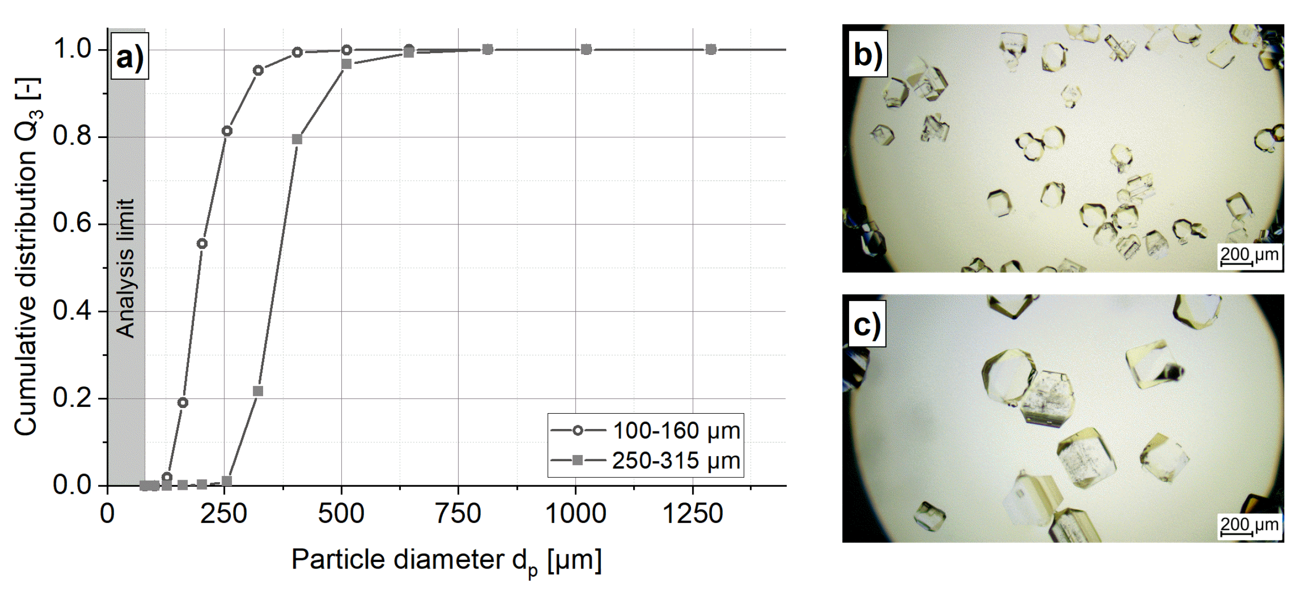
Flow map validation is conducted at a suitable operating point at the transition between two qualitative suspension states. As no suspension is expected in the investigated operating region of $n_{ATC}$ = 4–50 ${\min }^{-1}$ for sieve fraction 250–315 μm ($d_{mod}=364\mathsf{\mu }$m), sieve fraction 100–160 μm ($d_{mod}=182\mathsf{\mu }$m) is selected for the experiment. For this particle size, the transition from fully horizontally distributed (yellow) to a vertically distributed suspension state (dotted green) is estimated at Shield’s parameter $\mathsf{\Theta }=35$ or rotational speed $n_{ATC}=40{\min }^{-1}$. Solid content $w_{solid}$ is not considered in the developed flow map (compare Equations (17) and (18)). Thus, the selected operating point is investigated for two solid contents (compare Section 2.2) to exclude potential impacts.

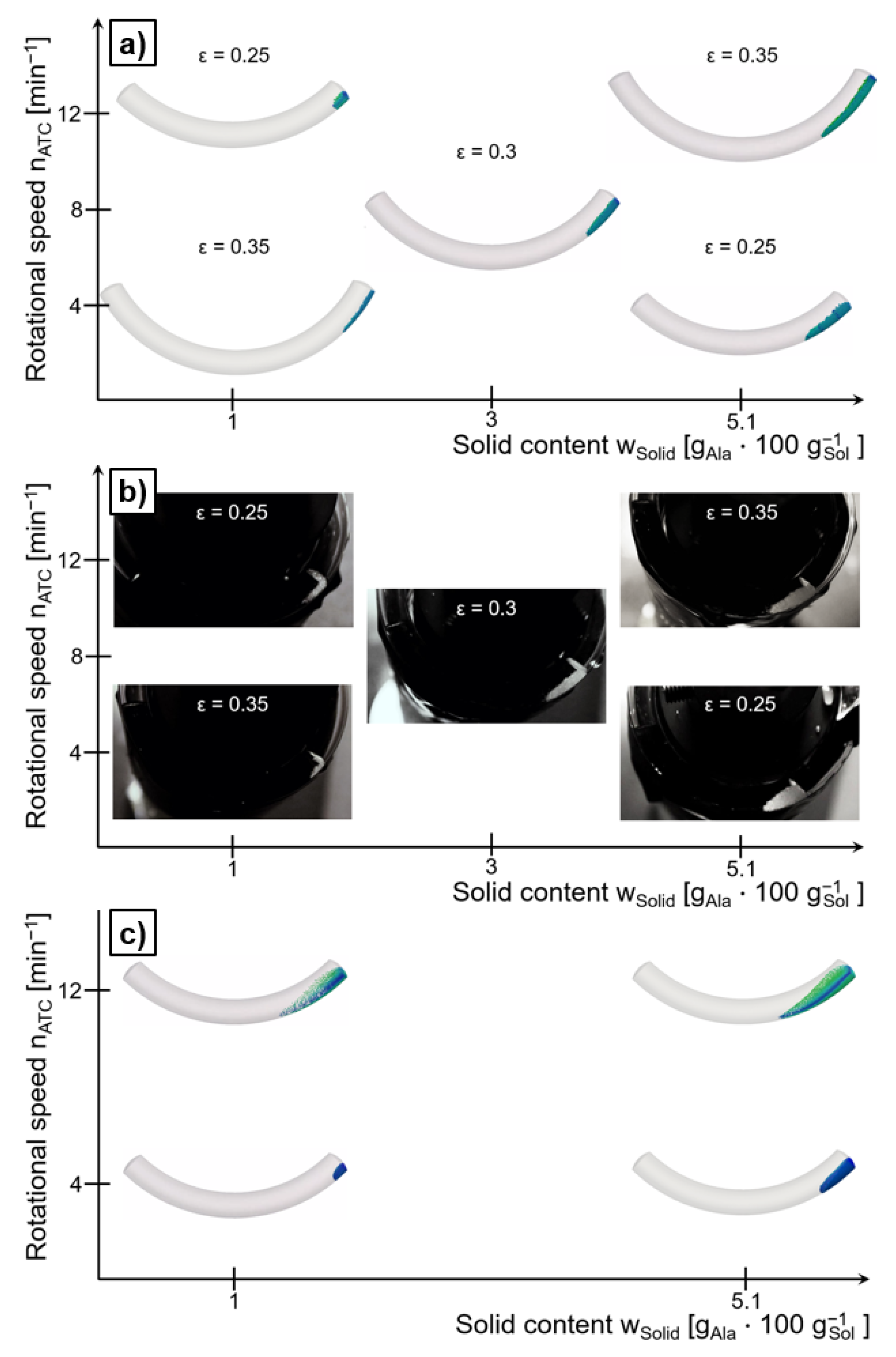
Figure 13 illustrates the suspension state at the selected operating point.

For the lower solid content (Figure 13a), particles are horizontally distributed as predicted. Furthermore, the particles are almost completely vertically distributed, thus the qualitative suspension state is close to homogeneous suspension. In addition, a particle recirculation vortex is visible at the rear half of the slug that was also calculated in the CFD simulations presented in Figure 9b. For the higher solid content (Figure 13b), the particles are no longer recognizable individually but rather seem homogeneously distributed in both directions. In this case, the higher solid content leads to particle overlapping. Thus, differences in particle distribution are difficult to record by camera. Nevertheless, higher suspension states might be reached by increasing the solid content due to particle swarm effects.

Overall, the observed suspension behavior in the validation experiments was better than expected, as almost homogeneous suspension (green) was reached at the selected operating point. This deviation reveals the suitability of the combination of the selected dimensionless numbers. The supplemental information gained from hydrodynamics with ratio $D{n}^{\ast }/Dn$ is beneficial to describe the flow enhancement through Dean vortices. For operating point $n_{ATC}=40{\min }^{-1}$, for example, radial mixing is twice as fast as angular mixing already. As a consequence, suspension quality is improved as well.

6. Conclusions and Outlook

A study to characterize hydrodynamics and suspension behavior in the small-scale Archimedes Tube Crystallizer (ATC) was conducted. To set up a flow map for the ATC, a five-step roadmap was introduced. In this approach, Computational Fluid Dynamics (CFD) simulations and experiments were integrated with dimensionless numbers to reduce experimental and simulative effort by conducting only target-oriented investigations. The flow map developed can be applied to estimate operating parameters for a selected material system and ATC design based on the targeted crystal product size.

For a continuous cooling crystallization process in the ATC, low rotational speeds may be required to achieve the necessary residence time for sufficient crystal growth. However, the required residence time is strongly dependent on the crystal growth rates of the material system. In general, by increasing the coiled tube diameter, larger particles can be obtained with sufficient suspension as well. Nevertheless, the required qualitative suspension state to avoid agglomeration in a cooling crystallization has yet to be determined.

In the future, a dimensional analysis should be conducted to develop dimensionless numbers that include both mixing and material-specific effects, such as solid content and particle shape. In addition, the CFD simulation tool developed in this contribution could be extended with a suitable population balance model to describe interrelations between suspension behavior and agglomeration. Thereby, the simulations could be enriched to include particle size distributions and further particle effects.