Magnetic Field and Dilution Effects on the Phase Diagrams of Simple Statistical Models for Nematic Biaxial Systems

Abstract

We use a simple statistical model to investigate the effects of an applied magnetic field and of the dilution of site elements on the phase diagrams of biaxial nematic systems, with an emphasis on the stability of the Landau multicritical point. The statistical lattice model consists of intrinsically biaxial nematogenic units, which interact via a Maier–Saupe potential, and which are characterized by a discrete choice of orientations of the microscopic nematic directors. According to previous calculations at zero field and in the absence of dilution, we regain the well-known sequence of biaxial, uniaxial, and disordered structures as the temperature is increased, and locate the Landau point. We then focus on the topological changes induced in the phase diagram by the application of an external magnetic field, and show that the Landau point is destabilized by the presence of an applied field. On the other hand, in the absence of a field, we show that only a quite strong dilution of nematic sites is capable of destabilizing the Landau point.

1. Introduction

In a number of recent investigations [1,2,3,4,5,6], we have performed some calculations for simple statistical lattice models to characterize the biaxial structures in liquid crystalline systems. These statistical models are based on fully-connected Maier–Saupe pair interactions, with a restricted choice of orientational degrees of freedom. They are amenable to detailed calculations, and have been shown to account for most of the qualitative features of the nematic phase diagrams, including the well-known sequences of biaxial nematic, uniaxial nematic, and isotropic structures, as the temperature is raised. At a special value of temperature and of a parameter gauging the degree of biaxiality, model calculations point out the existence of a highly symmetric Landau multicritical point, with a direct transition from a biaxial nematic to an isotropic phase.

In this work, we revisit the same simplified lattice models with a view to perform detailed calculations to investigate the effects produced by an applied field and by the dilution of nematogenic elements. Besides assuming a generalized form of the Maier–Saupe interactions between nematogenic units on a lattice site, we still make a discrete choice of the orientations of the microscopic nematic directors. This special choice, which is reminiscent of an old work of Zwanzig to treat the Onsager model of rigid cylinders, has also been shown to lead to the well-known first-order transition between simple uniaxial nematic and isotropic phases.

The effects of a magnetic field on the phase diagram of nematogenic molecules exhibiting biaxial phases have been the subject of a number of investigations over the years. For micellar lyotropic systems such as potassium laurate/1-decanol/water mixtures, in which shape anisotropy of the micelles is presumably strongly dependent on the temperature and on the concentration of the various components, the existence of a biaxial nematic phase is known since the pioneering work of Yu and Saupe [7]. Besides the biaxial phase, these systems also exhibit rod-like and disk-like uniaxial nematic phases, and, in general, upon heating, these uniaxial phases exhibit a discontinuous transition to an isotropic phase. Nevertheless, the three nematic phases and the isotropic phase become equal at the Landau multicritical point. In the neighborhood of the Landau point, experiments performed for three different values of concentration [8] show that application of a magnetic field turns the transition between the rod-like uniaxial and the isotropic phases into a crossover, while preserving the discontinuous nature of the transition between the disk-like uniaxial and the isotropic phases.

For mineral lyotropic systems, the combination of an intrinsic magnetic moment and a negative anisotropy of the magnetic susceptibility leads to a very strong induced magnetic birefringence [9] and to phase separation into a uniaxial nematic and a biaxial nematic due to entropic effects associated with polydispersity [10].

In thermotropic systems, prompted by experimental results [11] for bent-core, intrinsically biaxial molecules with an essentially fixed shape, there have been studies on the combined effect of biaxiality and a magnetic field on the temperature of the first-order uniaxial to a paranematic phase transition, on the stability of the various phases, and on the presence of multicritical points [11,12,13,14,15,16]. In particular, within the phenomenological Landau–de Gennes theory, Mukherjee and Rahman [13] have identified the destabilization of the Landau point and its splitting into one critical and two tricritical points.

In the present work, we go beyond the analysis of a Landau expansion. As we start from a microscopic statistical model, we are able to perform calculations to analyze the global phase diagram, which includes considerations on the stability of the Landau multicritical point and also illustrations of the behavior of the uniaxial and biaxial order parameters as temperature and degree of biaxiality are changed.

On the other hand, our motivation for investigating the effects of dilution is purely theoretical, as we would like to check whether the phase diagram of our simple model survives in the presence of an ingredient that is inescapable in the real world. Our results show that this is indeed the case, making clear that representing a fluid by a lattice model does not introduce any artifacts in our obtained phase diagrams.

In Section 2, we define the statistical model in terms of a quite general and elegant two-tensor formalism, proposed [17] by Sonnet, Virga, and Durand (SVD), and which includes all physically reasonable pair interactions between nematogenic elements. With a discrete choice of the microscopic directors, this model Hamiltonian is restricted to a six-state model, which we dub SVD6. Furthermore, we choose a relation between two interaction parameters, the “geometric-mean condition”, which preserves the main features of the phase diagrams, and which has been widely used in the area. We obtain a number of results for the phase diagram of this SVD6 model, in terms of temperature T and a parameter $\mathsf{\Delta }$, which comes from the geometric-mean condition and provides a form of gauging the degree of biaxiality. In particular, we locate the Landau multicritical point. In Section 3, we discuss the inclusion of an external field in the SVD6 Hamiltonian with the geometric-mean condition. The effects of a magnetic field come from an intricate competition between the magnetic free energy, the entropy and the interactions between nematogens, which can be fully accounted for by the elementary statistical model. In general, the presence of an external field breaks the symmetry necessary to stabilize the Landau point. Except for the very special circumstances of a fully isotropic diamagnetic susceptibility, the main result is the splitting of the transition lines and the disappearance of the Landau multicritical point. We then turn to the study of the effects of dilution. In Section 4, we use the SVD6 model, with the recourse to the geometric-mean condition, to show that the presence of dilution, as far as it is not a strong dilution, does not introduce any qualitative changes with respect to the initial phase diagrams. However, in the zero-field limit and for quite large dilutions, the Landau point turns into a first-order transition, which is similar to the behavior of the critical line in a strongly diluted Ising ferromagnet.

2. The SVD Model

The Hamiltonian representing the interactions between the nematogens in the mean-field SVD model [17] can be written as

$${\mathcal{H}}_{\mathrm{SVD}}=-\frac{A}{2V}\sum _{\mu ,\nu \in \left\{x,y,z\right\}}\left[{\left(\sum _{i=1}^V{q}_i^{\mu \nu }\right)}^2+2\gamma \left(\sum _{i=1}^V{q}_i^{\mu \nu }\right)\left(\sum _{i=1}^V{b}_i^{\mu \nu }\right)+\lambda {\left(\sum _{i=1}^V{b}_i^{\mu \nu }\right)}^2\right],$$

(1)

in which the parameter $A>0$ gauges the interaction between nematogens, the dimensionless parameters $\gamma$ and $\lambda$ are responsible for a dependence of that interaction on the relative orientation of the nematogens, and V is the number of nematogens, while $q_i^{\mu \nu }$ and $b_i^{\mu \nu }$, with $\mu ,\nu \in \{1,2,3\}$, are the components of two traceless tensors associated with the ith nematogen. Explicitly, for a generic nematogen with principal axes along the unit vectors ${\widehat{n}}_1$, ${\widehat{n}}_2$ and ${\widehat{n}}_3$, we have

$$\mathbf{q}=\frac{3}{2}{\widehat{n}}_1\otimes {\widehat{n}}_1-\frac{1}{2}\mathbf{I}\mathrm{and}\mathbf{b}=\frac{3}{2}\left({\widehat{n}}_2\otimes {\widehat{n}}_2-{\widehat{n}}_3\otimes {\widehat{n}}_3\right),$$

(2)

$\mathbf{I}$ being the $3\times 3$ identity matrix.

For our simplified model, we restrict the directors to point along the Cartesian axes [18,19], so that each nematogen takes only six distinct states, defining a new Hamiltonian

$${\mathcal{H}}_{\mathrm{SVD}6}=-\frac{A}{2V}\sum _{\alpha \in \left\{x,y,z\right\}}\left[{\left(\sum _{i=1}^V{q}_i^{\alpha \alpha }\right)}^2+2\gamma \left(\sum _{i=1}^V{q}_i^{\alpha \alpha }\right)\left(\sum _{i=1}^V{b}_i^{\alpha \alpha }\right)+\lambda {\left(\sum _{i=1}^V{b}_i^{\alpha \alpha }\right)}^2\right].$$

(3)

Labeling the states of a generic nematogen as ${\zeta }^{\left(k\right)}$, $k\in \left\{1,2,3,4,5,6\right\}$, the values of the diagonal components of the tensors $\mathbf{q}$ and $\mathbf{b}$, as well as of the z component of the first principal axis are given in

Table 1. Values of the diagonal components of the tensors q and b and of the z component of the principal axes of a generic nematogen in the six possible states ${\zeta }^{\left(k\right)}$ of the restricted model.

k	${\mathit{q}}^{\mathbf{xx}}$	${\mathit{b}}^{\mathbf{xx}}$	${\mathit{q}}^{\mathbf{yy}}$	${\mathit{b}}^{\mathbf{yy}}$	${\mathit{q}}^{\mathbf{zz}}$	${\mathit{b}}^{\mathbf{zz}}$	${\left({\mathit{n}}_1^{\mathit{z}}\right)}^2$	${\left({\mathit{n}}_2^{\mathit{z}}\right)}^2$	${\left({\mathit{n}}_3^{\mathit{z}}\right)}^2$
1	$-\frac{1}{2}$	$\frac{3}{2}$	$-\frac{1}{2}$	$-\frac{3}{2}$	1	0	1	0	0
2	$-\frac{1}{2}$	$-\frac{3}{2}$	$-\frac{1}{2}$	$\frac{3}{2}$	1	0	1	0	0
3	$-\frac{1}{2}$	$\frac{3}{2}$	1	0	$-\frac{1}{2}$	$-\frac{3}{2}$	0	0	1
4	$-\frac{1}{2}$	$-\frac{3}{2}$	1	0	$-\frac{1}{2}$	$\frac{3}{2}$	0	1	0
5	1	0	$-\frac{1}{2}$	$\frac{3}{2}$	$-\frac{1}{2}$	$-\frac{3}{2}$	0	0	1
6	1	0	$-\frac{1}{2}$	$-\frac{3}{2}$	$-\frac{1}{2}$	$\frac{3}{2}$	0	1	0

. Further restricting ourselves to the case $\lambda ={\gamma }^2$, the widely used geometric-mean condition [20,21], Equation (3) can be written as

$${\mathcal{H}}_{\mathrm{SVD}6}=-\frac{A}{2V}\sum _{\alpha \in \left\{x,y,z\right\}}{\left[\sum _{i=1}^V\left(q_i^{\alpha \alpha }+\gamma b_i^{\alpha \alpha }\right)\right]}^2.$$

(4)

As further discussed in Section 3, the parameter $\gamma$ appearing in the last expression can be interpreted as a simplified measure of the intrinsic biaxiality of the nematogens. The effect of $\gamma$ on the interaction energies under different relative orientations of a pair of nematogens replaces the entropic effects due to the different excluded volumes associated with these orientations for a pair of hard biaxial polyhedra, which, in the case of strong shape anisotropy, can also lead to the spontaneous appearance of stable biaxial phases [22].

3. Effects of a Magnetic Field

In order to consider the effects of a magnetic field, we add to the Hamiltonian of our simplified model the interactions of the nematogens with a uniform and constant field $\overrightarrow{H}=H\widehat{z}$ applied along the z axis in the laboratory frame [23]. We then write

$$\mathcal{H}={\mathcal{H}}_{\mathrm{SVD}6}-\frac{1}{2}\sum _{i=1}^V\sum _{j=1}^3{\chi }_j{\left(\overrightarrow{H}·{\widehat{n}}_{j,i}\right)}^2,$$

(5)

in which ${\chi }_j$ gauges the coupling with the magnetic field when the jth principal axis ${\widehat{n}}_j$ of an object lies along the field direction, and the index i runs over all objects. In view of the fact that, even under the geometric-mean condition, there are in general different interaction energies associated with distinct relative orientations of the principal axes of a pair of nematogens, no symmetry should be expected between field effects associated with choices of the sets of parameters $\left\{{\chi }_1,{\chi }_2,{\chi }_3\right\}$ such as $\left\{\chi ,0,0\right\}$, $\left\{0,\chi ,0\right\}$ and $\left\{0,0,\chi \right\}$.

The partition function Z of the model can be evaluated by introducing an auxiliary diagonal tensor $\mathbf{Q}=\mathrm{diag}\left\{Q_{xx},Q_{yy},Q_{zz}\right\}$ via three Gaussian identities which allow us to eliminate the quadratic terms arising from Equation (4), yielding

$$\begin{array}{cc}\hfill Z=\sum _{\left\{\zeta \right\}}{e}^{-\beta \mathcal{H}}=& {\left(\frac{\beta AV}{2\pi }\right)}^{3/2}\sum _{\left\{\zeta \right\}}\int \left[d{Q}_{\alpha \alpha }\right]exp\left\{-\frac{\beta AV}{2}\sum _{\alpha }{Q}_{\alpha \alpha }^2\right.\hfill \\ \hfill +& \left.\sum _{\alpha ,i}\beta A{Q}_{\alpha \alpha }\left(q_i^{\alpha \alpha }+\gamma b_i^{\alpha \alpha }\right)+\frac{\beta H^2}{2}\sum _{i,j}{\chi }_j{\left(n_{j,i}^z\right)}^2\right\},\hfill \end{array}$$

(6)

in which $\left[d{Q}_{\alpha \alpha }\right]=d{Q}_{xx}d{Q}_{yy}d{Q}_{zz}$ and $\beta =T^{-1}$ is the inverse temperature (we use a system of units for which Boltzmann’s constant $k_B=1$). Evaluating the sums over the nematogen index i and the states of each nematogen, we obtain

$$Z={\left(\frac{\beta AV}{2\pi }\right)}^{3/2}\int \left[d{Q}_{\alpha \alpha }\right]exp\left\{-\beta V\psi \left(\mathbf{Q}\right)\right\},$$

(7)

with

$$\psi \left(\mathbf{Q}\right)=\frac{A}{2}\sum _{\alpha }{Q}_{\alpha \alpha }^2-Tln2-Tln\varphi \left(\mathbf{Q}\right)$$

(8)

and

$$\begin{array}{cc}\hfill \varphi \left(\mathbf{Q}\right)& =e^{\frac{3}{2}\beta A{Q}_{xx}+\frac{1}{4}\beta \left({\chi }_2+{\chi }_3\right)H^2}cosh\left[\frac{3\beta A\gamma }{2}\left(Q_{yy}-Q_{zz}\right)-\frac{\beta \left({\chi }_2-{\chi }_3\right)H^2}{4}\right]\hfill \\ \hfill & +e^{\frac{3}{2}\beta A{Q}_{yy}+\frac{1}{4}\beta \left({\chi }_2+{\chi }_3\right)H^2}cosh\left[\frac{3\beta A\gamma }{2}\left(Q_{zz}-Q_{xx}\right)+\frac{\beta \left({\chi }_2-{\chi }_3\right)H^2}{4}\right]\hfill \\ \hfill & +e^{\frac{3}{2}\beta A{Q}_{zz}+\frac{1}{2}\beta {\chi }_1{H}^2}cosh\left[\frac{3\beta A\gamma }{2}\left(Q_{xx}-Q_{yy}\right)\right].\hfill \end{array}$$

(9)

The partition function can be evaluated by means of the steepest descent method. The equilibrium states correspond to those values $〈\mathbf{Q}〉$ of the tensor $\mathbf{Q}$ that minimize the functional $\psi \left(\mathbf{Q}\right)$. As these values are such that $\mathbf{Q}$ is traceless, we can write

$$〈\mathbf{Q}〉=\left(\begin{array}{ccc}-\frac{1}{2}\left(S+\eta \right)& 0& 0\\ 0& -\frac{1}{2}\left(S-\eta \right)& 0\\ 0& 0& S\end{array}\right),$$

(10)

in which S and $\eta$ play the roles of order parameters associated with the uniaxial and biaxial nematic phases, respectively. Noticing that at the mean-field level $〈\mathbf{Q}〉$ can be identified with $〈\mathit{q}+\gamma \mathit{b}〉$, we also have

$$〈\mathbf{Q}〉=\frac{3}{2}\left[〈{\widehat{n}}_1\otimes {\widehat{n}}_1〉+\gamma \left(〈{\widehat{n}}_2\otimes {\widehat{n}}_2〉-〈{\widehat{n}}_3\otimes {\widehat{n}}_3〉\right)\right]-\frac{1}{2}\mathbf{I}.$$

(11)

Substituting Equation (10) in Equation (8) we obtain

$$\psi \left(S,\eta \right)=\frac{3A}{4}{S}^2+\frac{A}{4}{\eta }^2-Tln2-Tln\varphi \left(S,\eta \right),$$

(12)

with

$$\begin{array}{cc}\hfill \varphi \left(S,\eta \right)& =e^{-\frac{3}{4}\beta A\left(S+\eta \right)+\frac{1}{4}\beta \left({\chi }_2+{\chi }_3\right)H^2}cosh\left[\frac{\beta A\mathsf{\Delta }}{4}\left(\eta -3S\right)-\frac{\beta \left({\chi }_2-{\chi }_3\right)H^2}{4}\right]\hfill \\ \hfill & +e^{-\frac{3}{4}\beta A\left(S-\eta \right)+\frac{1}{4}\beta \left({\chi }_2+{\chi }_3\right)H^2}cosh\left[\frac{\beta A\mathsf{\Delta }}{4}\left(\eta +3S\right)+\frac{\beta \left({\chi }_2-{\chi }_3\right)H^2}{4}\right]\hfill \\ \hfill & +e^{\frac{3}{2}\beta AS+\frac{1}{2}\beta {\chi }_1{H}^2}cosh\left(\frac{\beta A\mathsf{\Delta }}{2}\eta \right).\hfill \end{array}$$

(13)

Notice that in the above equations we introduced a biaxiality parameter $\mathsf{\Delta }=3\gamma$ so that we can compare our phase diagrams with the one obtained at zero field by Boccara, Medjani and De Seze [24]. If, for the sake of comparison, we assume that the traceless part of the inertia tensor and the $\mathit{q}+\gamma \mathit{b}$ tensor of an object are proportional to each other, we may interpret that, as $\mathsf{\Delta }$ is increased, the shape of the nematogen changes from calamitic (“rod-like”) uniaxial for $\mathsf{\Delta }=0$, to strongly biaxial for $\mathsf{\Delta }=1$, and finally to discotic (“disk-like”) uniaxial for $\mathsf{\Delta }=3$ (see the appendix in [4]). In this paper, we always work in the interval $0\le \mathsf{\Delta }\le 3$.

Minimizing Equation (12) we arrive at the state equations

$$\begin{array}{c}{\displaystyle \frac{\partial \psi }{\partial S}}={\displaystyle \frac{3A}{2}S-T\frac{\partial ln\varphi }{\partial S}}=0\\ {\displaystyle \frac{\partial \psi }{\partial \eta }}={\displaystyle \frac{A}{2}\eta -T\frac{\partial ln\varphi }{\partial \eta }}=0\end{array}$$

(14)

If there are multiple solutions to Equation (14), the equilibrium state corresponds to the solution with the smallest value of $\psi \left(S,\eta \right)$. At high temperatures and at zero field, there is an isotropic, disordered solution $S=\eta =0$. At lower temperatures, depending on the choice of $\mathsf{\Delta }$ and $\chi H^2$, there may appear uniaxial solutions, for which $\eta =0\ne S$, and biaxial solutions, for which $S\ne 0$ and $\eta \ne 0$. At zero field, due to the six-fold symmetry of the problem, there are degenerate solutions for the ordered phases, so that for every uniaxial solution $\left(S,\eta \right)=\left(S_0,0\right)$ there are equivalent solutions $\left(S,\eta \right)=\left(-\frac{1}{2}{S}_0,\pm \frac{3}{2}{S}_0\right)$. Of course, these do not correspond to biaxial solutions, which are not three-fold but six-fold degenerate. In fact, for each pair of biaxial solutions $\left(S_0,\pm {\eta }_0\right)$, with $\eta \ne 0$, there are equivalent solutions $\left(-\frac{1}{2}{S}_0\mp \frac{1}{2}{\eta }_0,\frac{3}{2}{S}_0\mp \frac{1}{2}{\eta }_0\right)$ and $\left(-\frac{1}{2}{S}_0\pm \frac{1}{2}{\eta }_0,-\frac{3}{2}{S}_0\mp \frac{1}{2}{\eta }_0\right)$. In the biaxial phase, comparison of Equations (10) and (11) in the $T\to 0$ limit indicates that the zero-field values of $\eta$ range from $\eta =-max\left\{\mathsf{\Delta },(\mathsf{\Delta }+3)/2\right\}$ to $\eta =max\left\{\mathsf{\Delta },(\mathsf{\Delta }+3)/2\right\}$. When plotting the values of S and $\eta$ in Figure 1, Figure 2 and Figure 3, we select for each choice of $\mathsf{\Delta }$ and T the solution that provides the clearest distinction between the phases.

Phase boundaries and multicritical points can be determined by the behavior of $\psi \left(S,\eta \right)$ and its derivatives at the solutions of Equation (14).

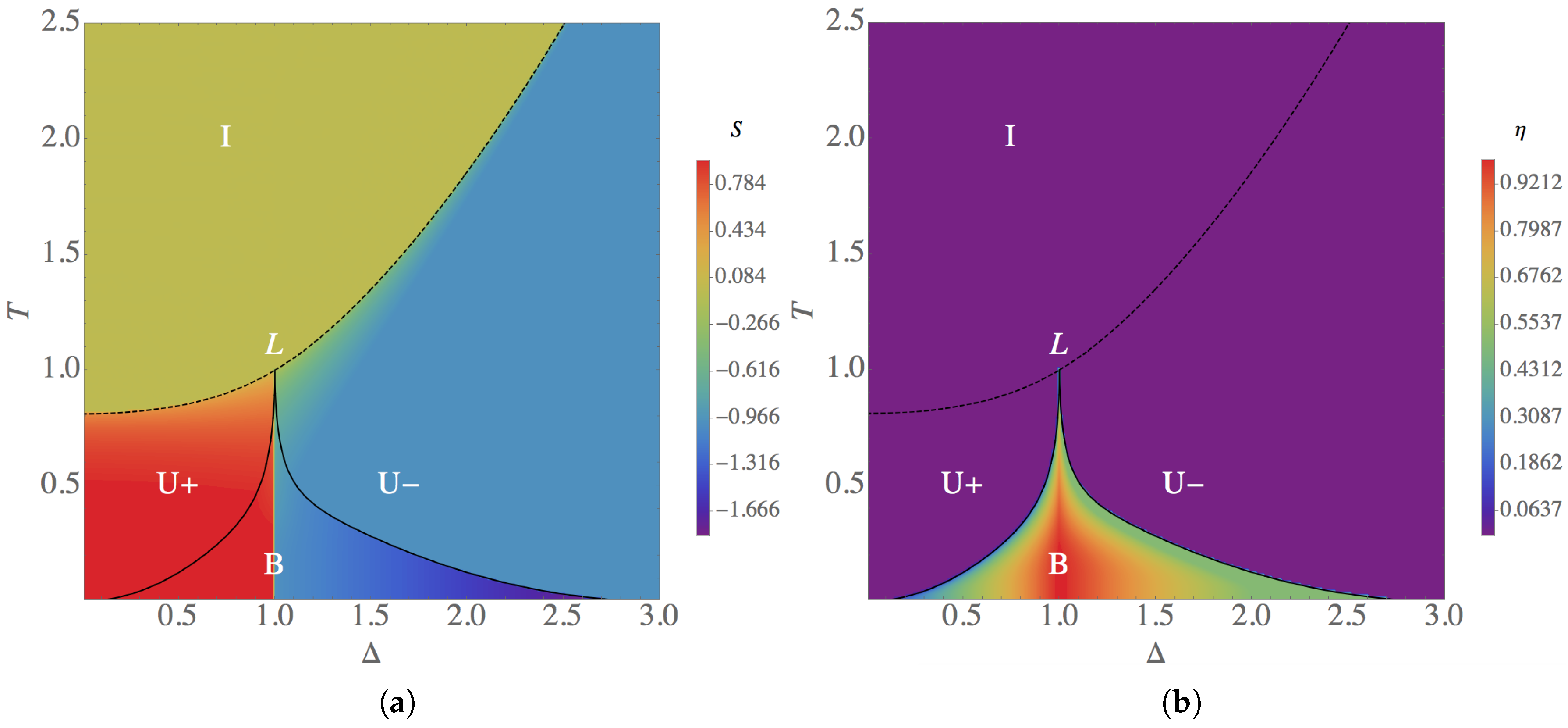
3.1. Behavior at Zero Field

We first offer a short review of the phase diagram at zero field ($H=0$), shown in Figure 1 and already discussed in [4,5,24].

When $\mathsf{\Delta }=0$, nematogens are intrinsically (calamitic) uniaxial, so that no biaxial phase is expected. Therefore, there is only a first-order transition between the uniaxial and the isotropic phases, which occurs at the temperature for which

$${\left.\frac{\partial \psi }{\partial S}\right|}_{\left(S_0,0\right)}=0\mathrm{and}\psi \left(S_0,0\right)=\psi \left(0,0\right).$$

(15)

As the biaxiality parameter $\mathsf{\Delta }$ is increased, a biaxial solution appears at a sufficiently small temperature. For fixed $\mathsf{\Delta }$, the temperature corresponding to the continuous transitions between the biaxial and the uniaxial phases is obtained from

$${\left.\frac{\partial \psi }{\partial S}\right|}_{\left(S_1,0\right)}={\left.\frac{{\partial }^2\psi }{\partial {\eta }^2}\right|}_{\left(S_1,0\right)}=0.$$

(16)

The lines of first-order uniaxial-isotropic and continuous biaxial-uniaxial transitions meet at the Landau multicritical point $\left({\mathsf{\Delta }}_L,T_L\right)$, the location of which is determined by the conditions

$${\left.\frac{{\partial }^2\psi }{\partial S^2}\right|}_{\left(0,0\right)}={\left.\frac{{\partial }^3\psi }{\partial S^3}\right|}_{\left(0,0\right)}=0,$$

(17)

derived by noticing that at that point $S_0$ and $S_1$ both tend smoothly to zero. For $H=0$, the above equations reduce to

$$\beta A\left({\mathsf{\Delta }}^2+3\right)-4={\beta }^2{A}^2\left({\mathsf{\Delta }}^2-1\right)=0,$$

(18)

so that, measuring T in units of the energy scale A, the solution to Equation (17) is

$$\left({\mathsf{\Delta }}_L,T_L\right)=\left(1,1\right).$$

(19)

Further increasing the value of $\mathsf{\Delta }$, the temperature of the biaxial–uniaxial transition decreases, becoming zero again at $\mathsf{\Delta }=3$, when the nematogen is once more a (discotic) uniaxial object. At the intermediate-temperature uniaxial phases, the uniaxial order parameter is positive ($S_0>0$) if $\mathsf{\Delta }<{\mathsf{\Delta }}_L$ and negative ($S_0<0$) if $\mathsf{\Delta }>{\mathsf{\Delta }}_L$.

We note that this phase diagram qualitatively agrees with the one obtained from computer simulations of a hard biaxial ellipsoid fluid, as a function of the shape anisotropy of the particles [25]. It also reproduces various aspects of phase diagrams of a variety of lyotropic systems [7,26,27,28,29], regarding their nematic phases.

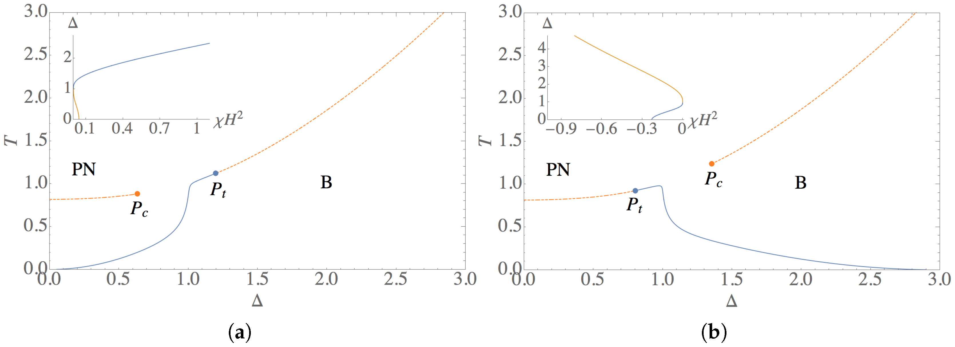
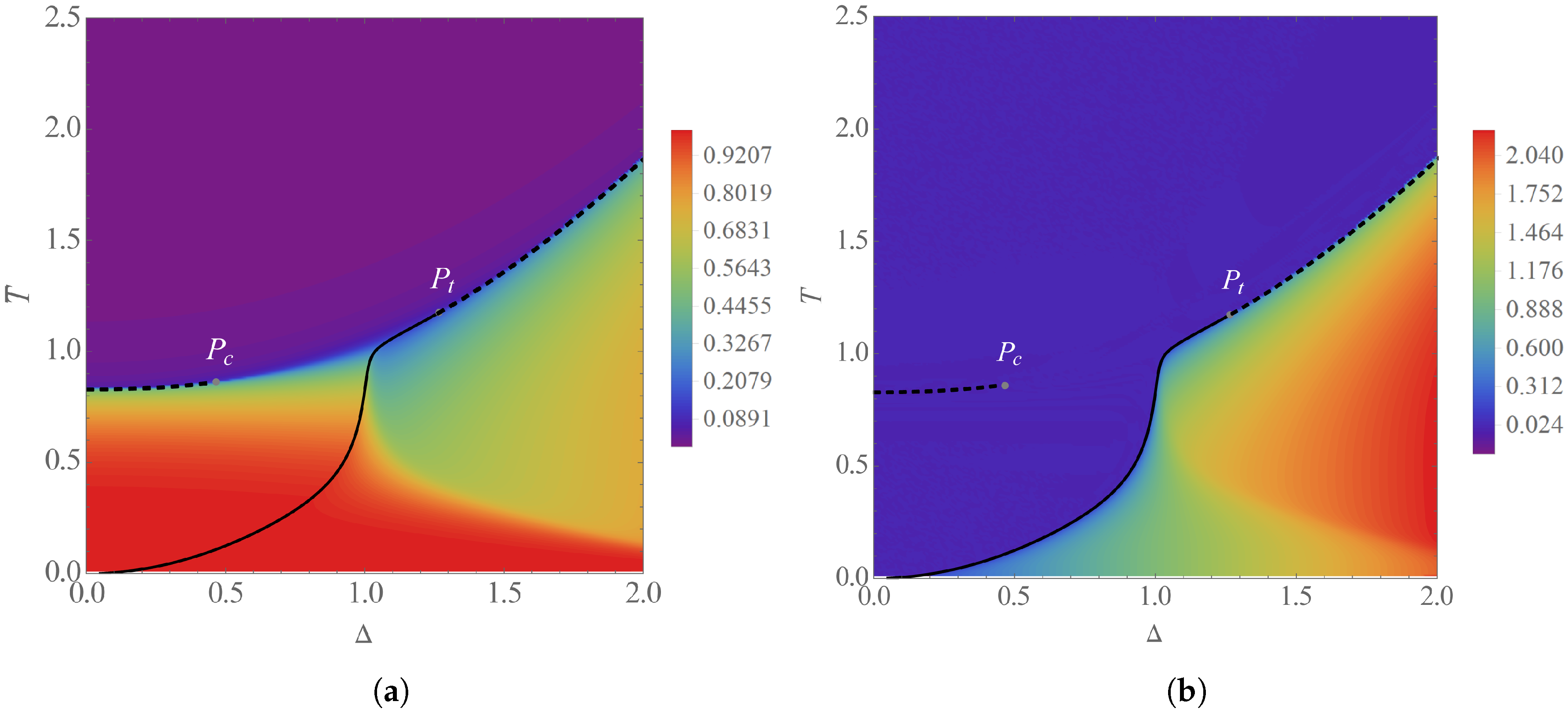
3.2. Phase Diagrams in a Field

The effect of a magnetic field is the result of an intricate competition between the magnetic free energy, the entropy and the mutual interactions between nematogens, as dictated by the geometric-mean condition.

The first noticeable effect of a nonzero field is the disappearance of the Landau point, except for the fully symmetric choice ${\chi }_1={\chi }_2={\chi }_3$, which makes all three principal axes of a nematogen equally likely to lie parallel to the field, having the sole effect of globally shifting all energy levels. This can be checked by fixing H and one of ${\chi }_j$, say ${\chi }_2$, and solving for $\mathsf{\Delta },$ $\beta A$, ${\chi }_1$ and ${\chi }_3$ the conditions in Equation (17) supplemented by

$${\left.\frac{\partial \psi }{\partial S}\right|}_{\left(0,0\right)}=0\mathrm{and}{\left.\frac{{\partial }^2\psi }{\partial {\eta }^2}\right|}_{\left(0,0\right)}=0,$$

(20)

the latter conditions being necessary for a continuous transition from a biaxial phase to a stable isotropic phase at a candidate Landau point. The only solution ever obtained is $\mathsf{\Delta }=1$, $\beta A=1$ and ${\chi }_1={\chi }_2={\chi }_3$, irrespective of the value of the field.

Nonetheless, for the special choice ${\chi }_2<{\chi }_1={\chi }_3$, which makes the ${\widehat{n}}_2$ principal axis of a nematogen less likely to lie perpendicular to the field, while making the ${\widehat{n}}_1$ and ${\widehat{n}}_3$ principal axes equally likely to lie parallel to the field, the isotropic phase is stable at a point fulfilling the conditions in Equation (17), although the second condition in Equation (20) is not satisfied.

As a typical example of the phase diagram in the presence of a field, let us consider the case ${\chi }_1\equiv \chi \ne 0$ and ${\chi }_2={\chi }_3=0$, which is representative of regime $\left|{\chi }_1\right|>\left|{\chi }_2\right|,\left|{\chi }_3\right|$. With this choice, the isotropic phase does not minimize the free energy at any finite temperature, being replaced by a paranematic phase in which $\eta =0$ but S takes a small but nonzero value. This can be rationalized as follows. Assuming $\chi >0$, it can be checked that the magnetic energy of a nematogen is minimized when the principal axes ${\widehat{n}}_1$ is parallel to the field direction z. From Equations (10) and (11), taking into account that ${〈{\widehat{n}}_j\otimes {\widehat{n}}_j〉}^{zz}=〈{\left(n_j^z\right)}^2〉$ and noticing that in a nonzero field the symmetry between $〈{\left(n_1^z\right)}^2〉$, $〈{\left(n_2^z\right)}^2〉$ and $〈{\left(n_3^z\right)}^2〉$ is explicitly broken, making $〈{\left(n_3^z\right)}^2〉=〈{\left(n_2^z\right)}^2〉<\frac{1}{3}$ and $〈{\left(n_1^z\right)}^2〉>\frac{1}{3}$ at high temperatures, it is clear that $S=〈Q_{zz}〉>0$. Likewise, assuming $\chi <0$, so that the magnetic energy of a nematogen is minimized when the principal axes ${\widehat{n}}_1$ is perpendicular to the field direction z, at high temperatures we have $〈{\left(n_3^z\right)}^2〉=〈{\left(n_2^z\right)}^2〉>\frac{1}{3}$ and $〈{\left(n_1^z\right)}^2〉<\frac{1}{3}$, so that $S=〈Q_{zz}〉<0$.

The general aspect of the phase diagram for both $\chi >0$ and $\chi <0$ is shown in Figure 2. In both cases, the Landau point disappears to give rise to a pair of multicritical points: a simple critical point signaling the end of a first-order transition line between the uniaxial and the paranematic phases (which are actually a single phase, in much the same way as the liquid and gaseous phases in simple fluids) and a tricritical point separating regions of first-order and continuous transitions between a biaxial phase and the paranematic phase. The dependence of the uniaxial and biaxial order parameters on $\mathsf{\Delta }$ and T is illustrated in Figure 3, for the case $\chi >0$. Notice the extension of the biaxial phase towards the region occupied, at zero field, by the discotic uniaxial phase.

The conditions for locating a first-order transition between the uniaxial and the paranematic phases are

$${\left.\frac{\partial \psi }{\partial S}\right|}_{\left(S_0,0\right)}={\left.\frac{\partial \psi }{\partial S}\right|}_{\left(S_0^{\prime },0\right)}=0\mathrm{and}\psi \left(S_0,0\right)=\psi \left(S_0^{\prime },0\right),$$

(21)

and at the associated critical point the solutions $S_0$ and $S_0^{\prime }$ become degenerate, so that

$${\left.\frac{{\partial }^2\psi }{\partial S^2}\right|}_{\left(S_0,0\right)}={\left.\frac{\partial \psi }{\partial S}\right|}_{\left(S_0,0\right)}=0.$$

(22)

A first-order transition between the biaxial and the paranematic phases occurs for

$${\left.\frac{\partial \psi }{\partial \eta }\right|}_{\left(S_2,{\eta }_2\right)}={\left.\frac{\partial \psi }{\partial S}\right|}_{\left(S_2,{\eta }_2\right)}={\left.\frac{\partial \psi }{\partial S}\right|}_{\left(S_0^{\prime },0\right)}=0\mathrm{and}\psi \left(S_2,{\eta }_2\right)=\psi \left(S_0^{\prime },0\right),$$

(23)

while a continuous transition between those same phases satisfies

$${\left.\frac{\partial \psi }{\partial S}\right|}_{\left(S_0^{\prime },0\right)}={\left.\frac{{\partial }^2\psi }{\partial {\eta }^2}\right|}_{\left(S_0^{\prime },0\right)}=0.$$

(24)

Finally, the location of the tricritical point can be determined from the conditions

$${\left.\frac{\partial \psi }{\partial S}\right|}_{\left(S_0^{\prime },0\right)}={\left.\frac{d^2\psi }{d{\eta }^2}\right|}_{\left(S_0^{\prime },0\right)}={\left.\frac{d^4\psi }{d{\eta }^4}\right|}_{\left(S_0^{\prime },0\right)}=0.$$

(25)

Notice that these last conditions involve total derivatives of the free-energy functional with respect to $\eta$, which means that, while calculating those derivatives, $S_0^{\prime }$ is implicitly treated as a function of $\eta$.

The multicritical points originating from the destabilization of the Landau point become increasingly separated as the magnetic field becomes more intense, as the insets in Figure 2 show. In the limit of an infinite field, only a continuous biaxial-paranematic phase transition remains.

The existence of a tricritical point on the line of biaxial to paranematic phase transitions is compatible with the predictions of [16], which assumes a more restrictive pair interaction independent of a biaxiality parameter, as well as with those of [6], in which nematogens are intrinsically uniaxial. In the latter case, the located tricritical point is observed for $\chi <0$ and at the value of the magnetic field necessary for our tricritical point to reach the uniaxial limit $\mathsf{\Delta }=0$; see the inset in Figure 2b. This same qualitative behavior for the appearance of a tricritical point in the uniaxial-paranematic transition was predicted for hard rods or hard plates with $\chi <0$ [30].

Similarly, the critical field associated with a critical end point of the first-order transition line between the uniaxial and the paranematic phases, which has been observed for a fixed biaxiality parameter by various authors [6,11,12,15,31], corresponds to the value of the field, which makes our simple critical point reach the uniaxial limit $\mathsf{\Delta }=0$ for $\chi >0$; see the inset in Figure 2a. Again, the same qualitative behavior for the appearance of a critical end point in the uniaxial-paranematic transition was predicted for hard rods or hard plates with $\chi >0$ [32].

Assuming that the biaxiality parameter of a system shows little variation with temperature or the strength of the magnetic field, which would be reasonable for thermotropic liquid crystals, our results suggest that, starting from a biaxial phase and heating the system under a constant field up to the transition to the paranematic phase, the nature of that transition should change from first-order to continuous (or vice-versa, depending on the sign of $\chi$) at a certain value of the field, signaling the tricritical point. Estimating the value of that field would require an estimate of the biaxiality parameter $\mathsf{\Delta }$ for the system, under the assumption that the geometric mean condition is at least approximately applicable. We expect that lyotropic systems, for which presumably there is a significant dependence of the biaxiality parameter on both the temperature and the composition of the mixture [26,27,29], are better candidates for the observation of a tricritical point.

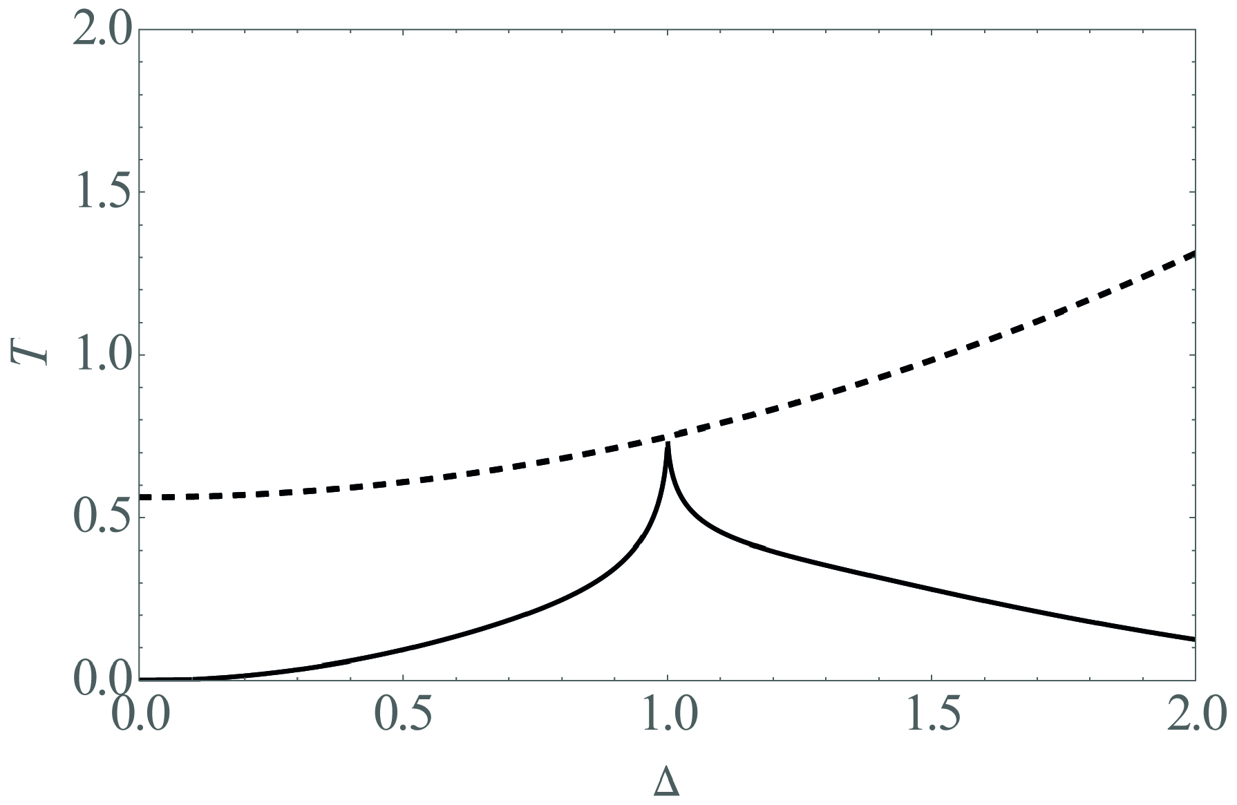
4. Introducing Dilution

Next we turn our attention to a “nematic lattice gas” model consisting of V sites, which can be either empty or occupied by a single object among $N\le V$ nematogens. This possibility can be represented at each site i by an occupation variable $t_i\in \left\{0,1\right\}$, and if the nematogens interact via the the extension of the Hamiltonian in Equation (4), the canonical partition function of the model at zero field can be written as

$$Z={\sum _{\left\{t\right\}}}^{\prime }\sum _{\left\{\zeta \right\}}exp\left\{\frac{\beta A}{2V}\sum _{\alpha \in \left\{x,y,z\right\}}{\left[\sum _{i=1}^V{t}_i\left(q_i^{\alpha \alpha }+\gamma b_i^{\alpha \alpha }\right)\right]}^2+\frac{\beta }{2}\sum _{i=1}^V\sum _{j=1}^3{t}_i{\chi }_j{(\overrightarrow{H}·{\widehat{n}}_{j,i})}^2\right\},$$

(26)

in which the prime in the summation over the set $\left\{t\right\}$ of occupation variables indicates that it should be restricted to those configurations for which

$$\sum _{i=1}^V{t}_i=N.$$

(27)

This restriction can be relaxed by introducing a chemical potential $\mu$ (not to be confused with the tensor index in Equation (1)) to enforce that the last equation be satisfied on average. We then have to calculate the grand-partition function

$$\mathsf{\Xi }=\sum _{\left\{t\right\}}\sum _{\left\{\zeta \right\}}exp\left\{\frac{\beta A}{2V}\sum _{\alpha \in \left\{x,y,z\right\}}{\left[\sum _{i=1}^V{t}_i\left(q_i^{\alpha \alpha }+\gamma b_i^{\alpha \alpha }\right)\right]}^2+\frac{\beta }{2}\sum _{i=1}^V\sum _{j=1}^3{t}_i{\chi }_j{\left(\overrightarrow{H}·{\widehat{n}}_{j,i}\right)}^2+\beta \mu \sum _{i=1}^V{t}_i\right\}.$$

(28)

Following the same strategy as in the previous section and introducing an auxiliary diagonal tensor $\mathbf{Q}=\mathrm{diag}\left\{Q_{xx},Q_{yy},Q_{zz}\right\}$ via three Gaussian identities, which allow us to eliminate the quadratic terms in $\mathsf{\Xi }$, we obtain

$$\begin{array}{cc}\hfill \mathsf{\Xi }=& {\left(\frac{\beta AV}{2\pi }\right)}^{3/2}\sum _{\left\{t\right\}}\sum _{\left\{\zeta \right\}}\int \left[d{Q}_{\alpha \alpha }\right]exp\left\{-\frac{\beta AV}{2}\sum _{\alpha }{Q}_{\alpha \alpha }^2+\right.\hfill \\ \hfill +& \left.\sum _{\alpha ,i}\beta A{Q}_{\alpha \alpha }{t}_i\left(q_i^{\alpha \alpha }+\gamma b_i^{\alpha \alpha }\right)+\frac{\beta }{2}\sum _{i,j}{t}_i{\chi }_j{\left(\overrightarrow{H}·{\widehat{n}}_{j,i}\right)}^2+\beta \mu \sum _{i=1}^V{t}_i\right\},\hfill \end{array}$$

(29)

and performing the sums over the nematogen index i, the occupation variables and the states of each nematogen, we can write

$$\mathsf{\Xi }={\left(\frac{\beta AV}{2\pi }\right)}^{3/2}\int \left[d{Q}_{\alpha \alpha }\right]exp\left\{-\beta V\mathsf{\Psi }\left(\mathbf{Q}\right)\right\},$$

(30)

with a grand functional

$$\mathsf{\Psi }\left(\mathbf{Q}\right)=\frac{A}{2}\sum _{\alpha }{Q}_{\alpha \alpha }^2-Tln\mathsf{\Phi }\left(\mathbf{Q}\right),$$

(31)

in which

$$\begin{array}{cc}\hfill \mathsf{\Psi }\left(\mathbf{Q}\right)& =6+2e^{\frac{3}{2}\beta A{Q}_{xx}+\frac{1}{4}\beta \left({\chi }_2+{\chi }_3\right)H^2+\beta \mu }cosh\left[\frac{3\beta A\gamma }{2}\left(Q_{yy}-Q_{zz}\right)-\frac{\beta \left({\chi }_2-{\chi }_3\right)H^2}{4}\right]\hfill \\ \hfill & +2e^{\frac{3}{2}\beta A{Q}_{yy}+\frac{1}{4}\beta \left({\chi }_2+{\chi }_3\right)H^2+\beta \mu }cosh\left[\frac{3\beta A\gamma }{2}\left(Q_{zz}-Q_{xx}\right)+\frac{\beta \left({\chi }_2-{\chi }_3\right)H^2}{4}\right]\hfill \\ \hfill & +2e^{\frac{3}{2}\beta A{Q}_{zz}+\frac{1}{2}\beta {\chi }_1{H}^2+\beta \mu }cosh\left[\frac{3\beta A\gamma }{2}\left(Q_{xx}-Q_{yy}\right)\right].\hfill \end{array}$$

(32)

Adopting again the parametrization in Equation (10) we can write the grand functional in terms of S and $\eta$, obtaining

$$\mathsf{\Psi }\left(S,\eta \right)=\frac{3A}{4}{S}^2+\frac{A}{4}{\eta }^2-Tln\mathsf{\Phi }\left(S,\eta \right),$$

(33)

with

$$\begin{array}{cc}\hfill \mathsf{\Phi }\left(S,\eta \right)& =2e^{-\frac{3}{4}\beta A\left(S+\eta \right)+\frac{1}{4}\beta \left({\chi }_2+{\chi }_3\right)H^2+\beta \mu }cosh\left[\frac{\beta A\mathsf{\Delta }}{4}\left(\eta -3S\right)-\frac{\beta \left({\chi }_2-{\chi }_3\right)H^2}{4}\right]\hfill \\ \hfill & +2e^{-\frac{3}{4}\beta A\left(S-\eta \right)+\frac{1}{4}\beta \left({\chi }_2+{\chi }_3\right)H^2+\beta \mu }cosh\left[\frac{\beta A\mathsf{\Delta }}{4}\left(\eta +3S\right)+\frac{\beta \left({\chi }_2-{\chi }_3\right)H^2}{4}\right]\hfill \\ \hfill & +2e^{\frac{3}{2}\beta AS+\frac{1}{2}\beta {\chi }_1{H}^2+\beta \mu }cosh\left(\frac{\beta A\mathsf{\Delta }}{2}\eta \right)+6.\hfill \end{array}$$

(34)

In the limit $\beta \mu \gg 1$, as expected for a fully occupied lattice, Equation (33) reduces to

$$\mathsf{\Psi }\left(S,\eta \right)=\psi \left(S,\eta \right)-\mu ,$$

(35)

in which $\psi \left(S,\eta \right)$ is given by Equation (12).

The equilibrium values of S and $\eta$ are obtained by minimizing $\mathsf{\Psi }\left(S,\eta \right)$ with respect to both variables at a fixed chemical potential, yielding the state equations

$$\begin{array}{c}{\displaystyle \frac{\partial \mathsf{\Psi }}{\partial S}}={\displaystyle \frac{3A}{2}S-T\frac{\partial ln\mathsf{\Psi }}{\partial S}}=0\\ {\displaystyle \frac{\partial \mathsf{\Psi }}{\partial \eta }}={\displaystyle \frac{A}{2}\eta -T\frac{\partial ln\mathsf{\Psi }}{\partial \eta }}=0\end{array},$$

(36)

and once again there may exist isotropic, uniaxial and biaxial solutions.

In the presence of a nonzero field, it is straightforward to show that for small dilution we recover the same qualitative results of Section 3 regarding the destabilization of the Landau point, which is replaced by a simple critical point and a tricritical point.

On the other hand, in the limit of zero field ($H=0$), to which we limit ourselves for the rest of this section, a Landau point occurs when

$${\left.\frac{{\partial }^2\mathsf{\Psi }}{\partial S^2}\right|}_{\left(0,0\right)}={\left.\frac{{\partial }^3\mathsf{\Psi }}{\partial S^3}\right|}_{\left(0,0\right)}=0.$$

(37)

The above condition on the third derivative yields ${\mathsf{\Delta }}_L=1$, while the remaining condition leads to

$$\left(\beta A-1\right)e^{\beta \mu }-1=0,$$

(38)

the solution of which defines a line of Landau points corresponding to a varying chemical potential. For $\beta \mu \gg 1$, we recover the result ${\beta }_{L}A=1$ obtained at zero field in Equation (19). As $\mu$ is reduced, the temperature corresponding to the solution of Equation (38) is also reduced, as it can be checked by calculating the implicit derivative of $\beta$ with respect to $\mu$ from Equation (38).

Besides having $\mathsf{\Delta }=1$ and fulfilling Equation (38), a true Landau point has to represent a stable isotropic phase. In the present case, this requires that this phase be a minimum rather than a saddle point of the grand functional. It turns out that, at the candidate Landau point, the second derivative of $\mathsf{\Psi }\left(S,\eta \right)$ with respect to $\eta$ is always zero at the isotropic phase $\left(S,\eta \right)=\left(0,0\right)$, but that the corresponding fourth derivative,

$${\left.\frac{{\partial }^4\mathsf{\Psi }}{\partial {\eta }^4}\right|}_{\left(0,0\right)}=\frac{27{\beta }^3{A}^4\left(1-e^{-\beta \mu }\right)}{8{\left(1+e^{-\beta \mu }\right)}^2},$$

(39)

changes from positive for $\mu >0$ to negative for $\mu <0$, indicating that the Landau point corresponds to a stable phase only if the chemical potential is nonnegative.

In order to obtain phase diagrams involving the concentration c of occupied sites rather than the chemical potential $\mu$, at every equilibrium point we need to solve for $\mu$ the equation

$$c=〈\frac{1}{V}\sum _{i=1}^V{t}_i〉=\frac{1}{\beta V}\frac{\partial }{\partial \mu }ln\mathsf{\Xi },$$

(40)

which is equivalent to solving

$$c=-{\left.\frac{\partial \mathsf{\Psi }}{\partial \mu }\right|}_{\left(S,\eta \right)}=\frac{\mathsf{\Phi }\left(S,\eta \right)-6}{\mathsf{\Phi }\left(S,\eta \right)},$$

(41)

with S and $\eta$ assuming their equilibrium values and $\mathsf{\Phi }\left(S,\eta \right)$ given by Equation (34).

In particular, at the Landau point the relation between $\mu$ and the concentration c is given by

$$c=\frac{e^{\beta \mu }}{1+e^{\beta \mu }},$$

(42)

indicating that the Landau point is stable if $c>\frac{1}{2}$ and unstable if $c<\frac{1}{2}$. Therefore, for small dilution the Landau point is always stable. In this limit, the phase diagram is qualitatively the same as in the fully packed limit, as illustrated in Figure 4.

5. Conclusions

We use a recently proposed two-tensor formalism, which is based on the physically acceptable pair interactions between nematogenic units, and assume a discrete set of orientations of the microscopic nematic directors, to write a six-state lattice Hamiltonian. The fully-connected version of this system is amenable to detailed statistical mechanics calculations. In the widely used geometric-mean approximation for the model parameters, we regain the well-known phase diagram of nematic biaxial systems, with sequences of biaxial-uniaxial-disordered phase transitions as temperature increases, and the appearance of a well-defined Landau multicritical point. We locate the transition lines and the position of the Landau multicritical point in terms of temperature and a parameter $\mathsf{\Delta }$ that gauges the degree of biaxiality.

With the addition of an external magnetic field, we show that, except in a quite unusual diamagnetic isotropic case, the topology of this phase diagram is entirely changed. Our calculations indicate that the Landau point can no longer exist. In the phase diagrams, in terms of temperature and the parameter $\mathsf{\Delta }$, we show that there appear a pair of multicritical points, and a simple critical point at the end of the first-order border between a uniaxial and a paranematic phase. Also, we show the onset of a tricritical point separating borders of first-order and continuous transitions between a biaxial and a paranematic phase. We expect that lyotropic systems, for which presumably there is a significant dependence of the biaxiality parameter on both the temperature and the composition of the mixture [26,27,29], are good candidates for the observation of both the simple critical point and the tricritical point. We point out that our predictions for $\chi >0$ are fully compatible with available experimental results for potassium laurate/1-decanol/water mixtures [8], which show, based on measurements performed at three distinct concentrations in the neighborhood of the Landau point, that the application of a magnetic field turns the transition between the rod-like uniaxial and the isotropic phases into a crossover, while preserving the discontinuous nature of the transition between the disk-like uniaxial and the isotropic phases. Locating the simple critical point and the tricritical point in this system would require some extremely fine tuning, but in principle it should be feasible.

On the other hand, in the presence of moderate dilution the zero-field phase diagram is essentially unchanged. For stronger dilution, however, the Landau point also disappears, which is very similar to a phenomenon associated with a dilute ferromagnet.

Finally, we stress that, from a formal point of view, our results are equally applicable to the situation in which a liquid crystal is subject to an electric rather than a magnetic field [33].

References

1. do Carmo, E.; Liarte, D.B.; Salinas, S.R. Statistical models of mixtures with a biaxial nematic phase. Phys. Rev. E 2010, 81, 062701. [Google Scholar] [CrossRef] [PubMed] [Green Version]
2. do Carmo, E.; Vieira, A.P.; Salinas, S.R. Phase diagram of a model for a binary mixture of nematic molecules on a Bethe lattice. Phys. Rev. E 2011, 83, 011701. [Google Scholar] [CrossRef] [PubMed] [Green Version]
3. Liarte, D.B.; Salinas, S.R. Enhancement of Nematic Order and Global Phase Diagram of a Lattice Model for Coupled Nematic Systems. Braz. J. Phys. 2012, 42, 261. [Google Scholar] [CrossRef] [Green Version]
4. Nascimento, E.S.; Henriques, E.F.; Vieira, A.P.; Salinas, S.R. Maier-Saupe model for a mixture of uniaxial and biaxial molecules. Phys. Rev. E 2015, 92, 062503. [Google Scholar] [CrossRef] [PubMed] [Green Version]
5. Nascimento, E.S.; Vieira, A.P.; Salinas, S.R. Lattice Statistical Models for the Nematic Transitions in Liquid-Crystalline Systems. Braz. J. Phys. 2016, 46, 664. [Google Scholar] [CrossRef] [Green Version]
6. Petri, A.; Salinas, S.R. Field-induced uniaxial and biaxial nematic phases in the Maier–Saupe–Zwanzig (MSZ) lattice model. Liquid Cryst. 2018, 45, 980–992. [Google Scholar] [CrossRef]
7. Yu, L.J.; Saupe, A. Observation of a Biaxial Nematic Phase in Potassium Laurate-1-Decanol-Water Mixtures. Phys. Rev. Lett. 1980, 45, 1000–1003. [Google Scholar] [CrossRef] [Green Version]
8. Melnik, G.; Photinos, P.; Saupe, A. Landau point on a nematic-isotropic transition line. Phys. Rev. A 1989, 39, 1597–1600. [Google Scholar] [CrossRef]
9. Lemaire, B.J.; Davidson, P.; Ferré, J.; Jamet, J.P.; Panine, P.; Dozov, I.; Jolivet, J.P. Outstanding Magnetic Properties of Nematic Suspensions of Goethite (α-FeOOH) Nanorods. Phys. Rev. Lett. 2002, 88, 125507. [Google Scholar] [CrossRef]
10. van den Pol, E.; Lupascu, A.; Diaconeasa, M.A.; Petukhov, A.V.; Byelov, D.V.; Vroege, G.J. Onsager Revisited: Magnetic Field Induced Nematic–Nematic Phase Separation in Dispersions of Goethite Nanorods. J. Phys. Chem. Lett. 2010, 1, 2174–2178. [Google Scholar] [CrossRef]
11. Ostapenko, T.; Wiant, D.B.; Sprunt, S.N.; Jákli, A.; Gleeson, J.T. Magnetic-Field Induced Isotropic to Nematic Liquid Crystal Phase Transition. Phys. Rev. Lett. 2008, 101, 247801. [Google Scholar] [CrossRef] [PubMed] [Green Version]
12. To, T.B.T.; Sluckin, T.J.; Luckhurst, G.R. Biaxiality-induced magnetic field effects in bent-core nematics: Molecular-field and Landau theory. Phys. Rev. E 2013, 88, 062506. [Google Scholar] [CrossRef] [PubMed] [Green Version]
13. Mukherjee, P.K.; Rahman, M. Isotropic to biaxial nematic phase transition in an external magnetic field. Chem. Phys. 2013, 423, 178. [Google Scholar] [CrossRef]
14. Aliev, M.; Ugolkova, E.; Kuzminyh, N. Effect of an external magnetic field on the phase behavior of the thermotropic melt of V-shaped molecules. J. Mol. Liquids 2019, 292, 111395. [Google Scholar] [CrossRef]
15. Matsuyama, A.; Arikawa, S.; Wada, M.; Fukutomi, N. Uniaxial and biaxial nematic phases of banana-shaped molecules and the effects of an external field. Liquid Cryst. 2019, 46, 1672. [Google Scholar] [CrossRef]
16. Mukherjee, P.K.; De, A.K.; Mandal, A. Mean-field theory of isotropic-uniaxial nematic-biaxial nematic phase transitions in an external field. Phys. Scr. 2019, 94, 025702. [Google Scholar] [CrossRef]
17. Sonnet, A.M.; Virga, E.G.; Durand, G.E. Dielectric shape dispersion and biaxial transitions in nematic liquid crystals. Phys. Rev. E 2003, 67, 061701. [Google Scholar] [CrossRef]
18. de Oliveira, M.J.; Figueiredo Neto, A.M. Reentrant isotropic-nematic transition in lyotropic liquid crystals. Phys. Rev. A 1986, 34, 3481. [Google Scholar] [CrossRef]
19. Sauerwein, R.A.; de Oliveira, M.J. Lattice model for biaxial and uniaxial nematic liquid crystals. J. Chem. Phys. 2016, 144, 194904. [Google Scholar] [CrossRef]
20. Luckhurst, G.R.; Zannoni, C.; Nordio, P.L.; Segre, U. A molecular field theory for uniaxial nematic liquid crystals formed by non-cylindrically symmetric molecules. Mol. Phys. 1975, 30, 1345. [Google Scholar] [CrossRef]
21. Luckhurst, G.R.; Naemura, S.; Sluckin, T.J.; Thomas, K.S.; Turzi, S.S. Molecular-field-theory approach to the Landau theory of liquid crystals: Uniaxial and biaxial nematics. Phys. Rev. E 2012, 85, 031705. [Google Scholar] [CrossRef] [PubMed]
22. Dussi, S.; Tasios, N.; Drwenski, T.; van Roij, R.; Dijkstra, M. Hard Competition: Stabilizing the Elusive Biaxial Nematic Phase in Suspensions of Colloidal Particles with Extreme Lengths. Phys. Rev. Lett. 2018, 120, 177801. [Google Scholar] [CrossRef] [PubMed] [Green Version]
23. Photinos, D.J. Alignment of biaxial nematics. In Biaxial Nematic Liquid Crystals: Theory, Simulation, and Experiment; Luckhurst, G.R., Sluckin, T.J., Eds.; Wiley: West Sussex, UK, 2015; p. 205. [Google Scholar]
24. Boccara, N.; Mejdani, R.; De Seze, L. Solvable model exhibiting a first-order phase transition. J. Phys. France 1977, 38, 149. [Google Scholar] [CrossRef]
25. Camp, P.J.; Allen, M.P. Phase diagram of the hard biaxial ellipsoid fluid. J. Chem. Phys. 1997, 106, 6681–6688. [Google Scholar] [CrossRef] [Green Version]
26. Figueiredo Neto, A.M.; Galerne, Y.; Levelut, A.M.; Liebert, L. Pseudo-lamellar ordering in uniaxial and biaxial lyotropic nematics: A synchrotron X-ray diffraction experiment. J. Phys. Lett. 1985, 46, 499. [Google Scholar] [CrossRef]
27. Galerne, Y.; Figueiredo Neto, A.M.; Liébert, L. Microscopical structure of the uniaxial and biaxial lyotropic nematics. J. Chem. Phys. 1987, 87, 1851–1856. [Google Scholar] [CrossRef]
28. Oliveira, E.A.; Liebert, L.; Neto, A.M.F. A new soap/detergent/water lyotropic liquid crystal with a biaxial nematic phase. Liquid Cryst. 1989, 5, 1669–1675. [Google Scholar] [CrossRef]
29. Akpinar, E.; Reis, D.; Figueiredo Neto, A.M. Effect of alkyl chain length of alcohols on nematic uniaxial-to-biaxial phase transitions in a potassium laurate/alcohol/K2SO4/water lyotropic mixture. Liquid Cryst. 2012, 39, 881–888. [Google Scholar] [CrossRef] [Green Version]
30. Varga, S.; Kronome, G.; Szalai, I. External field induced tricritical phenomenon in the isotropicnematic phase transition of hard non-spherical particle systems. Mol. Phys. 2000, 98, 911–915. [Google Scholar] [CrossRef]
31. Vause, C.A. Connection between the isotropic-nematic Landau point and the paranematic-nematic critical point. Phys. Lett. A 1986, 114, 485–490. [Google Scholar] [CrossRef]
32. Varga, S.; Jackson, G.; Szalai, I. External field induced paranematic–nematic phase transitions in rod-like systems. Mol. Phys. 1998, 93, 377–387. [Google Scholar]
33. Lelidis, I.; Durand, G. Electric-field-induced isotropic-nematic phase transition. Phys. Rev. E 1993, 48, 3822–3824. [Google Scholar] [CrossRef] [PubMed]
Figure 1. Phase diagram at zero field, in the T × Δ plane. The color code shows the behavior of (a) the uniaxial order parameter S, which is zero in the high-temperature isotropic phase (I), and (b) the biaxial order parameter η , which is nonzero only in the low-temperature biaxial (B) phase. Notice that at low and intermediate temperatures the value of S associated with the smallest equilibrium value of η changes sign along the line Δ = 1 on which the Landau point Δ L , T L = 1 , 1 is located. Solid (dashed) lines indicate continuous (first-order) transitions. The calamitic (U+) and discotic (U−) uniaxial phases are also indicated.
Crystals 10 00632 g001
Figure 2. Main plots: Phase diagrams in the presence of a field of intensity H = 0.1 , with the choice χ 1 χ 0 and χ 2 = χ 3 = 0 , both for χ = 1 (a) and χ = 1 (b). The Landau point is replaced by a simple critical point P c and a tricritical point P t . The regions corresponding to the paranematic (PN) and the biaxial (B) phases are also indicated. Insets: Dependence of the values of Δ at P c (orange curve) and P t (blue curve) on the product χ H 2 . Apart from small shifts produced by the field, a combined parametric T × Δ plot obtained from the values of T and Δ at P c and P t as χ H 2 is varied would closely follow the first-order lines in Figure 1.
Crystals 10 00632 g002
Figure 3. Phase diagram at a field H = 0.15 , with the choice χ 1 , χ 2 , χ 3 = 1 , 0 , 0 , in the T × Δ plane. The color code shows the behavior of (a) the uniaxial order parameter S, which is always nonzero in the paranematic phase, which extends up to high temperatures, and (b) the biaxial order parameter η , which is nonzero only in the biaxial phase, which now extends to intermediate temperatures when Δ > 1 . Notice that both S and η present a steep but nonsingular behavior in the region corresponding, at zero field, to the continuous transition between the biaxial and the discotic uniaxial phases.
Crystals 10 00632 g003
Figure 4. Zero-field phase diagram for the diluted model, when the concentration of nematogens corresponds to c = 0.75 . Notice the lower temperature at the Landau point and a slightly more asymmetrical uniaxial–biaxial transition line around the line Δ = 1 .
Crystals 10 00632 g004