1. Introduction
Through many decades, the Landau theory (LT) of phase transitions [
1,
2] (PTs) has proven to be one of the most valuable conceptual tools for understanding PTs of the group-subgroup type. In particular, the field of structural PTs abounds even with successful quantitative applications, and, for many classes of materials, complete collections of the corresponding coupling coefficients have been gathered in the literature (for ferroelectrics see, e.g., Appendix A of Ref. [
3]). Effects of spontaneous strain that generally accompany temperature-driven structural PTs are sufficiently parameterized in terms of infinitesimal strain tensor components defined with respect to a baseline, which is obtained by extrapolating the generally small thermal expansion changes of the high symmetry reference phase. The corresponding Landau potential then involves only terms up to harmonic order, and any temperature dependence of the relevant parameters (high symmetry phase elastic constants and other coupling constants) can usually be completely neglected [
4].
The situation changes drastically for high pressure phase transitions (HPPTs). Spontaneous strain components may still be numerically small, but they now must be defined with respect to a
P-dependent base line. The total strain measured with respect to the ambient pressure reference state must then be calculated from a nonlinear superposition of finite background and spontaneous strain (see Equation (
11) below). Furthermore, the Landau potential may be truncated beyond harmonic order only if calculated with respect to this
P-dependent elastic background reference system. Therefore, neither the elastic constants nor the other elastic couplings can be assumed to be
P-independent. In a high pressure context, clinging to the familiar infinitesimal strain Landau toolbox may result not only in a quantitatively, but also qualitatively completely erroneous description.
It is not easy to construct a mathematically consistent and yet practically useful version of Landau theory taking into account the inherent nonlinearities and anharmonic effects that accompany HPPTs. In recent years, however, such a theory, for which we have coined the name finite strain Landau theory (FSLT), has been successfully developed. FSLT constitutes a careful extension of Landau theory beyond coupling to infinitesimal strain, fully taking into account the nonlinear elastic effects at finite strain. Its capabilities have been demonstrated in a number of applications to HPPTs [
5,
6,
7,
8,
9,
10]. However, as it stands, the numerical scheme underlying FSLT is still quite involved, and many practical workers in the field of HPPTs may be hesitant to go through the mathematical hardships it seems to pose. It is the purpose of this paper to show that FSLT is drastically simplified by switching from a formulation in terms of Cartesian Lagrangian strains to one in terms of symmetry-adapted finite strains. The enormous reduction of overall complexity of the approach as well as the vastly reduced numerical requirements of our new version of FSLT are demonstrated on the example of the HPPT in the perovskite KMnF
3 (KMF).
2. Review of Experimental Results on the Cubic-to-Tetragonal Transition of KMF
In what follows, we focus on the antiferrodistortive high pressure phase transition of KMF from the cubic perovskite aristophase
to a tetragonal
phase at room temperature which was experimentally investigated in Ref. [
11] by X-ray diffraction up to
. Since the ambient pressure Landau theory also provides a limiting reference frame for the description of the high pressure transition, we start our discussion with a detailed survey of the corresponding Landau theory.
According to Ref. [
12], a similar transition observed at ambient pressure and temperature
is weakly first order but close to critical, and the mechanism underlying these transitions is the same as in the well-studied
cubic-to-tetragonal transition in strontium titanate, i.e., octahedral tilting with a critical wavevector at the
R-point of the cubic Brillouin zone. Furthermore, in Ref. [
12], it is argued that, even though a further structural transition to an orthorhombic phase related to further octahedral tilting at the
M-point of the Brillouin zone at
is accompanied by antiferromagnetism, this coincidence between structural and magnetic transition temperatures may just be accidental, and actually there seems to be essentially no coupling between structural and magnetic order parameters (OPs) for these transitions. In passing we note that at
there is a further transition to an orthorhombic canted ferromagnet [
12].
As discussed in Ref. [
12], the
symmetry reduction corresponds to the isotropy subgroup of the three-dimensional irreducible representation
of
with respect to the order parameter direction
, the corresponding Landau expansion to sixth order being
with volume and tetragonal symmetry-adapted strains
,
and bulk and longitudinal shear modulus related to the bare cubic elastic constants by
,
. Targeting a transition into a single tetragonal domain where
and
, we have
In a standard Landau approach, the coefficients
are assumed to be independent of temperature (and pressure), while for
A the ansatz
with
T-independent coefficients
is made and quantum saturation has been neglected [
13]. The elastic equilibrium conditions
and
amount to
with a background volume strain
Performing a Legendre transform yields the Gibbs potential
where
The values of coefficients
,
and
at
, which imply a first order phase transition at
, have been determined from caloric measurements by Salje and coworkers [
13]. In principle, numerical values for the OP-strain coupling coefficients
may be extracted from experimental data on the temperature evolution of spontaneous strains
. Unfortunately, however, for KMF, this is easier said than done. At room temperature, the thermal expansion data
of Ref. [
14] are observed to perfectly reproduce the value of the cubic lattice constant
at ambient pressure as determined in Ref. [
11]. However, the measurement data of thermal lattice parameter irregularities
around
(Refs. [
15,
16,
17,
18]) available in the literature appear to be in rather poor mutual agreement. As
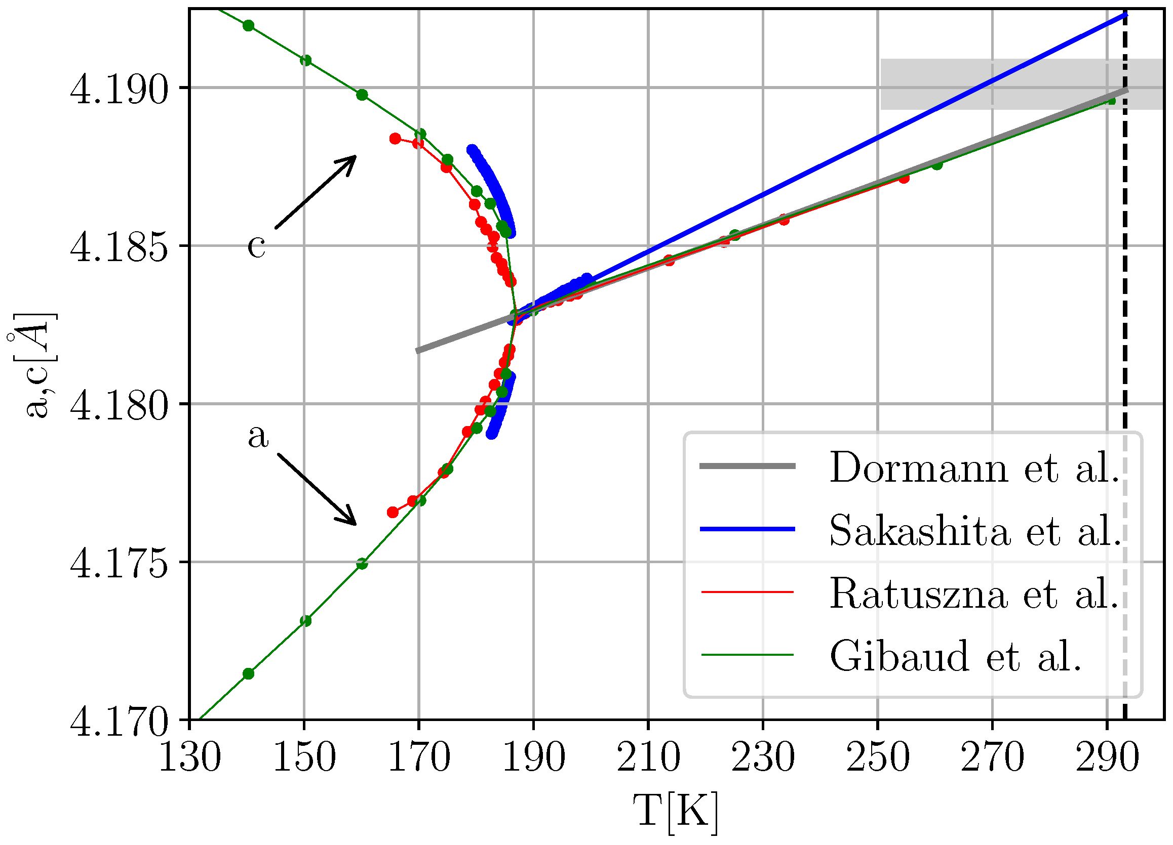
Figure 1 illustrates, while a discontinuous behavior of the lattice parameters is clearly visible in all three data sets, the absolute values of the measured unit cell parameters differ considerably, yet none of the data sets seem to be compatible with extrapolating the thermal expansion data of Ref. [
14].
Not unexpectedly, the agreement in relative splitting between the a-and c-axis in the tetragonal phase appears to be better, albeit far from perfect. Nevertheless, the cubic parts of the data of Refs. [
15,
18] exhibit slopes similar to the low temperature extrapolation of the thermal expansion data of Ref. [
14]. In order to be able to collapse the data onto a common “master set”, we thus shifted the data of Refs. [
15,
18] by constant absolute offsets to match the extrapolated baseline of Ref. [
14] in an optimal way, treating the seemingly more precise measurements of Sakashita et al. (Refs. [
16,
17]) as an outlier.
Figure 2 illustrates our results for a corresponding effort.
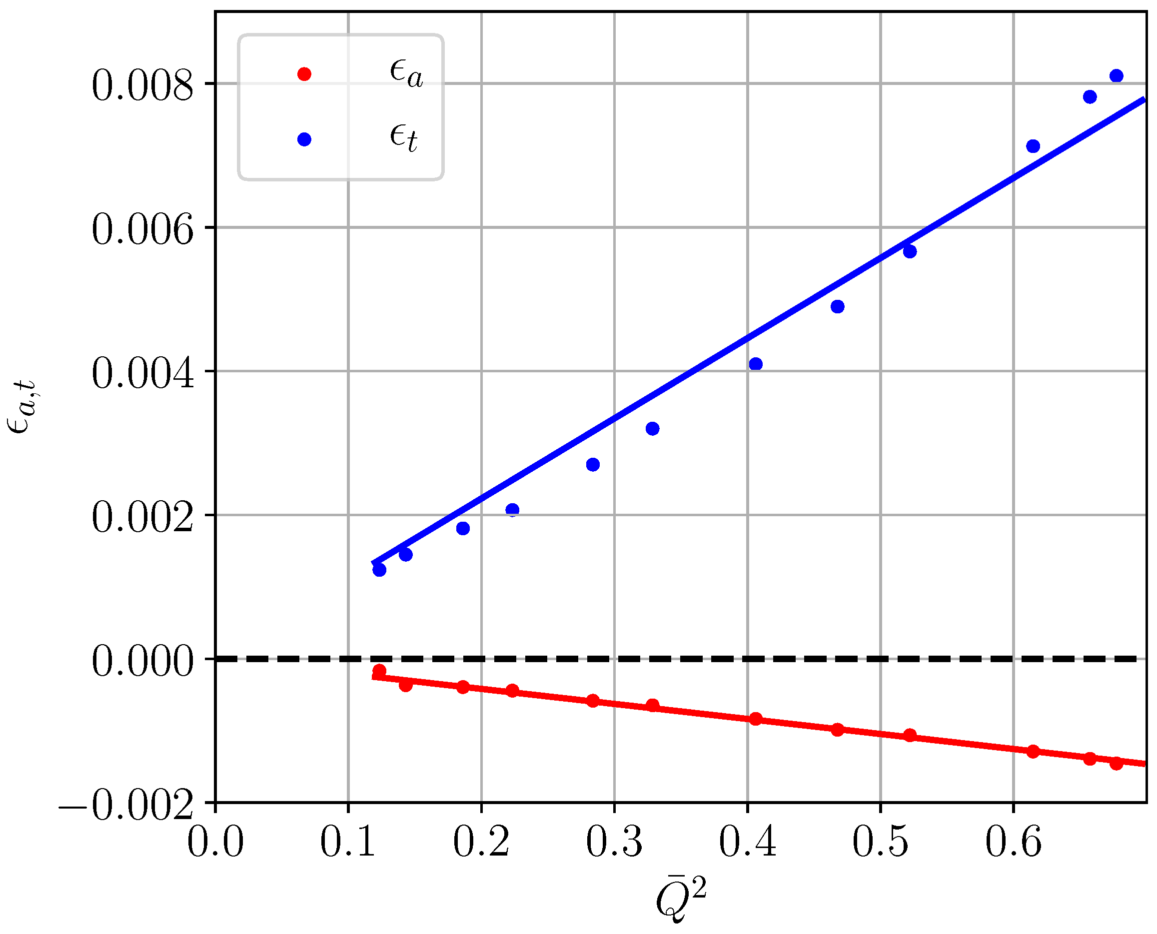
With a meaningful baseline
for unit cell parameters
in place, we calculate the spontaneous strain components
and
and thus the (infinitesimal) spontaneous volume and tetragonal strains
respectively. According to Equation (
4), when plotted against
at
,
and
should resemble straight lines with slopes
and
, respectively.
Figure 3 illustrates corresponding fits with results
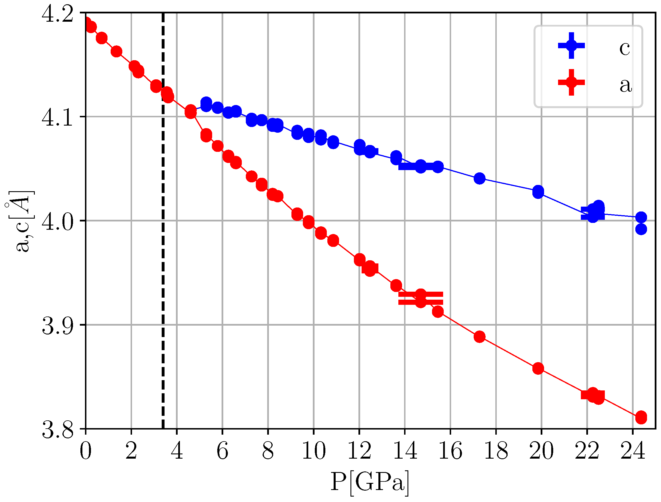
With the Landau theory of the temperature-driven transition at ambient pressure available, we are tempted to analyze the ambient temperature HPPT based on the same framework. In Ref. [
11], the variation of the pseudo-/cubic lattice constants of KMF under pressure at room temperature was measured with X-ray scattering (
Figure 4) and the cubic part of the data was fitted to a simple Murnaghan equation of state (EOS) with
and
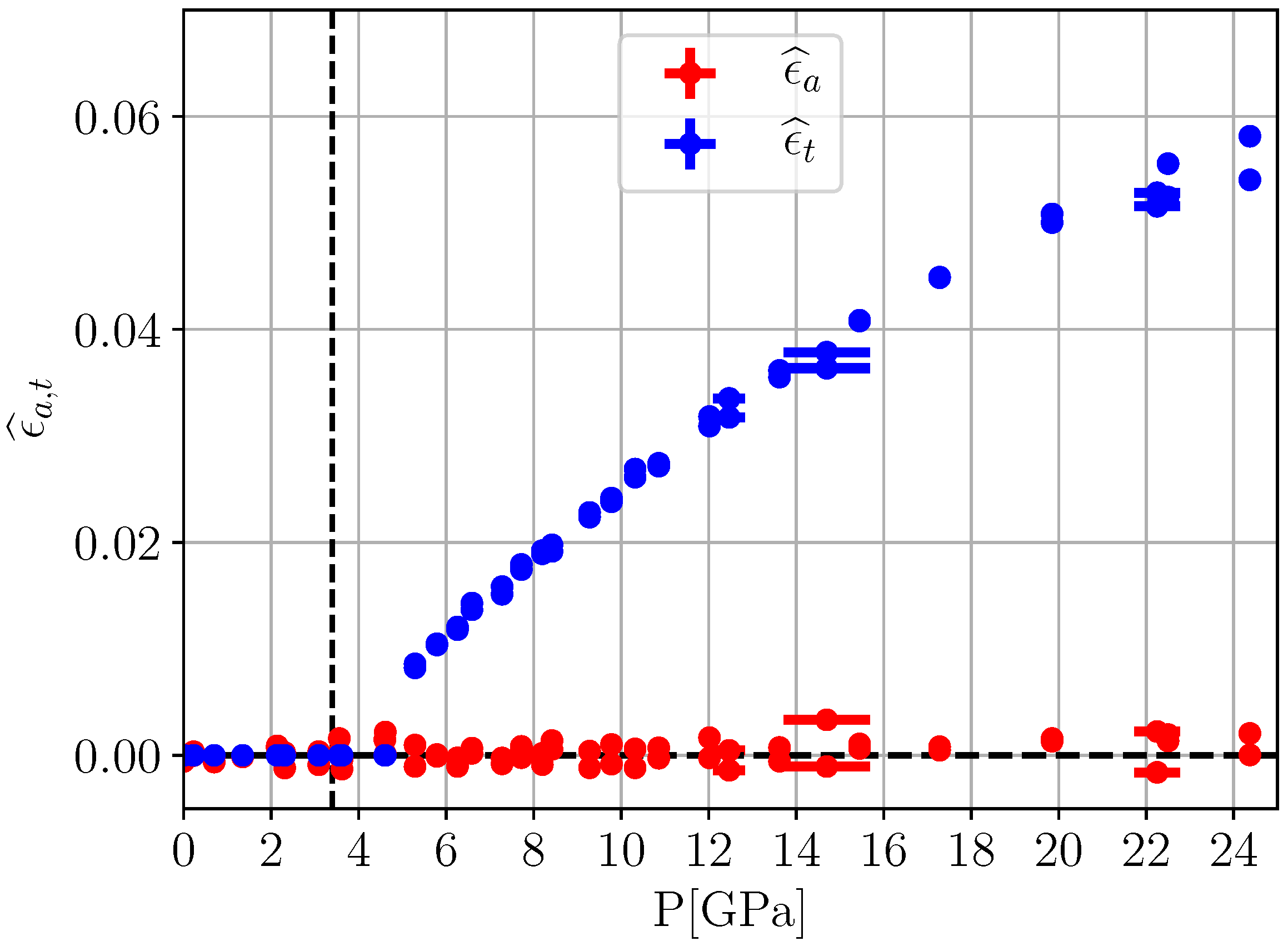
. This provides a baseline to determine (Lagrangian) spontaneous strains
(
Figure 5).
Comparing the thermal and pressure-induced spontaneous strains shown in
Figure 2 and
Figure 5, respectively, we note that there is some spontaneous thermal volume strain
while practically
for the pressure-induced case. Furthermore, even though it may be difficult to directly relate temperature and pressure scales, the pressure-induced tetragonal spontaneous strain
is observed to be roughly one order of magnitude larger than its thermal counterpart
. From the perspective of traditional Landau theory based on infinitesimal strain coupling, these findings are difficult to explain. Based on Equation (
4), there are in principle two ways to alter the magnitude of spontaneous strains. One may either change the value of the couplings
and
or find a mechanism to increase the magnitude of
which, of course, implicitly depends on all Landau coefficients. Since these are actually only known for
, one could assume a thermal drift in
towards zero to be responsible for the vanishing of
at room temperature (more than counteracting against the thermal drift of
which is generally expected to decrease with increasing
T). For the tetragonal strain, a similar mechanism seems to be difficult to conceive, however. On the one hand, we would need to increase
dramatically to explain the large values of
. On the other hand, Equation (
7b) indicates that such an increase would send parameter
to negative values much larger than those found for the thermal transition, resulting in a pronounced first order character of the HTTP. This, however, is not observed. The only remedy therefore seems to find a way to increase
. Calculated from a standard 2–4 Landau potential,
would be inversely proportional to
. This may explain why advocates of an orthodox Landau description frequently resort to assuming HPPT’s to be near a tricritical point, explicitly postulating some ad-hoc pressure dependence
induced somehow by unspecified higher order coupling effects.
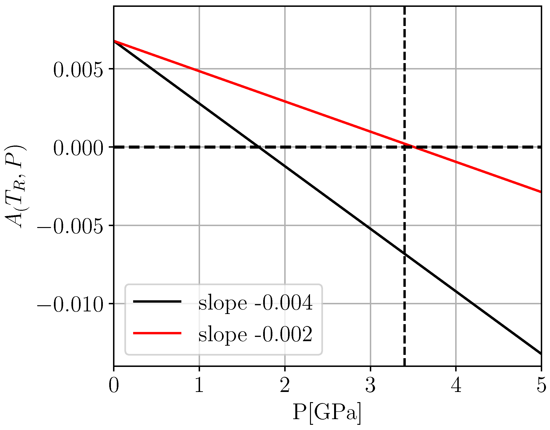
Further difficulties arise if we try to reconcile the observed value of
with the prediction of standard Landau theory. In Ref. [
11], a brute force fit based on the above assumptions of a second order transition close to a tricitical point produced an estimate of
. In principle, for a second order or slightly first order phase transition, this pressure should coincide or be somewhat lower than the pressure value
at which
vanishes at room temperature
. Unfortunately, however, this is incompatible with extrapolating the Landau parametrization of Hayward et al. [
19] to room temperature. In fact, inserting the parameter value (
10) into Equation (
7a) yields
, which is completely at odds with
as reported in Ref. [
11]. To reach this transition pressure at room temperature would require reducing our previous result
obtained at
by a full factor of 2 (cf.
Figure 6). However, even then, any unbiased reader should have a hard time believing that the bare data of
Figure 5 should indicate a continuous transition at
. In summary, we hope to have demonstrated that standard Landau theory is completely inadequate to describe the HPPT of KMF unless one is willing to sacrifice any numerical meaning to Landau theory, leaving us with all coupling parameters as essentially unknown and with ad hoc pressure dependencies at room temperature.
3. A Quick Review of FSLT
In a nutshell, in a generic high pressure experiment, a given crystal is observed to change under application of high hydrostatic pressure
P from an ambient pressure “laboratory” state
to a deformed state to be denoted as
with an accompanying total (Lagrangian) strain
. Frequently, a high pressure phase transition manifests itself in such an experiment through the observation of relatively small strain anomalies on top of a much larger “background strain” that in itself is unrelated to the actual transition. Recognizing that the concept of strain is always defined with respect to a chosen elastic reference state, in Ref. [
5], a corresponding background system
, defined as the (hypothetical) equilibrium state of the system with the primary OP clamped to remain zero, was introduced. Let
and
denote the deformation and Lagrangian strain tensors from
to
, respectively. The total strain
may then be disentangled as a nonlinear superposition
of the—generally large—Lagrangian background strain and a relatively small spontaneous strain
measured relative to the floating “background” reference state . Determining the proper background strain
in the resulting reference scheme
is thus a crucial step in correctly identifying the actual spontaneous strain, which in turn is mandatory in a successful application of the concepts of Landau theory. Effectively “subtracting” the elastic baseline, the strategy of FSLT therefore consists of setting up Landau theory
within the background reference system . Based on the reasonable assumption that a harmonic expansion with pressure-dependent elastic constants
suffices to capture the elastic energy originating exclusively from the relatively small spontaneous strain
, one arrives at the Landau free energy
where we have assumed a scalar OP
Q for simplicity, and
denotes the pure spontaneous strain-dependent elastic free energy at hydrostatic external stress
. For the pure OP potential part, we assume the traditional Landau expansion
with
P-dependent coefficients yet to be determined. In Ref. [
9], it was explicitly shown that the harmonic structure of
yields the equilibrium spontaneous strain
where the compliance tensor
is defined as the tensorial inverse of the so-called
Birch coefficients [
20,
21]
of the background system
which effectively take over the role of the elastic constants at finite strain. Furthermore, if we eliminate
from
by this formula, we obtain the renormalized pure OP potential
from which the equilibrium OP
can be determined by minimization.
Information on the
P-dependence of elastic constants
is usually available from density functional theory (DFT) or may be extracted from experimental measurements. At this stage, it therefore remains to relate the potential coefficients
and
, which are still defined with respect to the reference system
i.e.,
P-dependent. In a generic application of FSLT, however, one starts from knowledge of an ambient pressure Landau potential, i.e., the lowest order coefficients of the free energy
(defined at
) with
P-
independent coefficients are assumed to be known, which obviously places constraints on the possible
P-dependence of the above coefficients
and
. To explore the relations between the two set of coefficients defined in the
P-dependent background system
and the laboratory system
, we insert the nonlinear superposition relation (11) into (19) and compare coefficients. Following Ref. [
9], we content ourselves to just include OP-strain couplings of type
and obtain
in addition to the trivial relations
, where
.
The above parametrization scheme, although mathematically correct, is certainly not very convenient for applications in which the background reference state
is of high symmetry. For the most important example of a cubic high-symmetry phase, the above equations simplify considerable, since the deformation tensor
is diagonal, and so is the Lagrangian background strain
with
, which yields
These formulas are as far as we can get without committing to a specific set of irreducible representations that determine the symmetry-allowed couplings in the Landau potential. Since the background strains , they effectively represent a set of highly interrelated power series in powers of P. Unfortunately, this also comes with all the inherent drawbacks. On the one hand, going beyond the lowest order terms, which may be taken from an previously determined ambient pressure Landau potential, we are forced to truncate the above series at rather low order to limit the number of additional unknown parameters. Of course, such truncated series inevitable diverge for increasing values of P. In addition, if we want to employ the theory for the purpose of fitting experimental data, we would like to fix certain experimental observables, in particular the pressure at which vanishes. Given the above parametrization, this is obviously difficult to do.
In
Section 2, we have demonstrated the considerable structural simplification of a standard ambient pressure Landau approach upon replacing Cartesian strain tensors by symmetry-adapted strains. Remarkably, it turns out that, despite the additional complicated nonlinearities contained in Formulas (21a) and (21b), similar manipulations may also be carried out in FSLT and are found to yield equally substantial structural simplifications. In the rest of the paper, the resulting scheme will be derived and illustrated by describing the HPPT of KMF.
4. Symmetry-Adapted FSLT: The Cubic-to-Tetragonal HP Phase Transition of KMF
For
, we set
in accordance with
Equations (21a) and (21b) are then replaced by
Furthermore, we recall from nonlinear elasticity theory [
20] that for a cubic system the compliance tensor
and the bulk modulus
at finite pressure are related by
, while, for the longitudinal shear modulus,
the relation
holds. If we replace the Cartesian equilibrium spontaneous strain Components (
16) by their symmetry-adapted volume and tetragonal counterparts using these relations, they acquire the representations
Furthermore, it is easy to check the identity
which allows for similarly rewriting the renormalized potential
as
Combining these equations with Equations (24a) and (24b), we can summarize the symmetry-adapted parametrization of the coefficients of the renormalized Landau potential (
18), whose minimization determines the equilibrium OP
with
in addition to
, where we introduced the function
Note the close formal similarity of Equations (28a), (28b) and (
29) with their infinitesimal counterparts (7a) and (7b). In a generic application of this theory with cubic high symmetry, the lowest order Landau coefficients
and the lowest order strain-OP coupling coefficients
can be taken from an existing ambient pressure Landau theory. Furthermore, the (diagonal) background deformation components
and the resulting Lagrangian strain
may be determined by fitting a suitable EOS to the cubic unit cell volume data. Such a fit also immediately yields the pressure-dependent bulk modulus
. It is only for the pressure-dependence of the longitudinal shear modules
that we are truly forced to resort to additional input from DFT. To determine the EOS and the elastic constants of
, we have performed a series of fairly standard DFT calculations. We refer to
Appendix A for further details of these simulations.
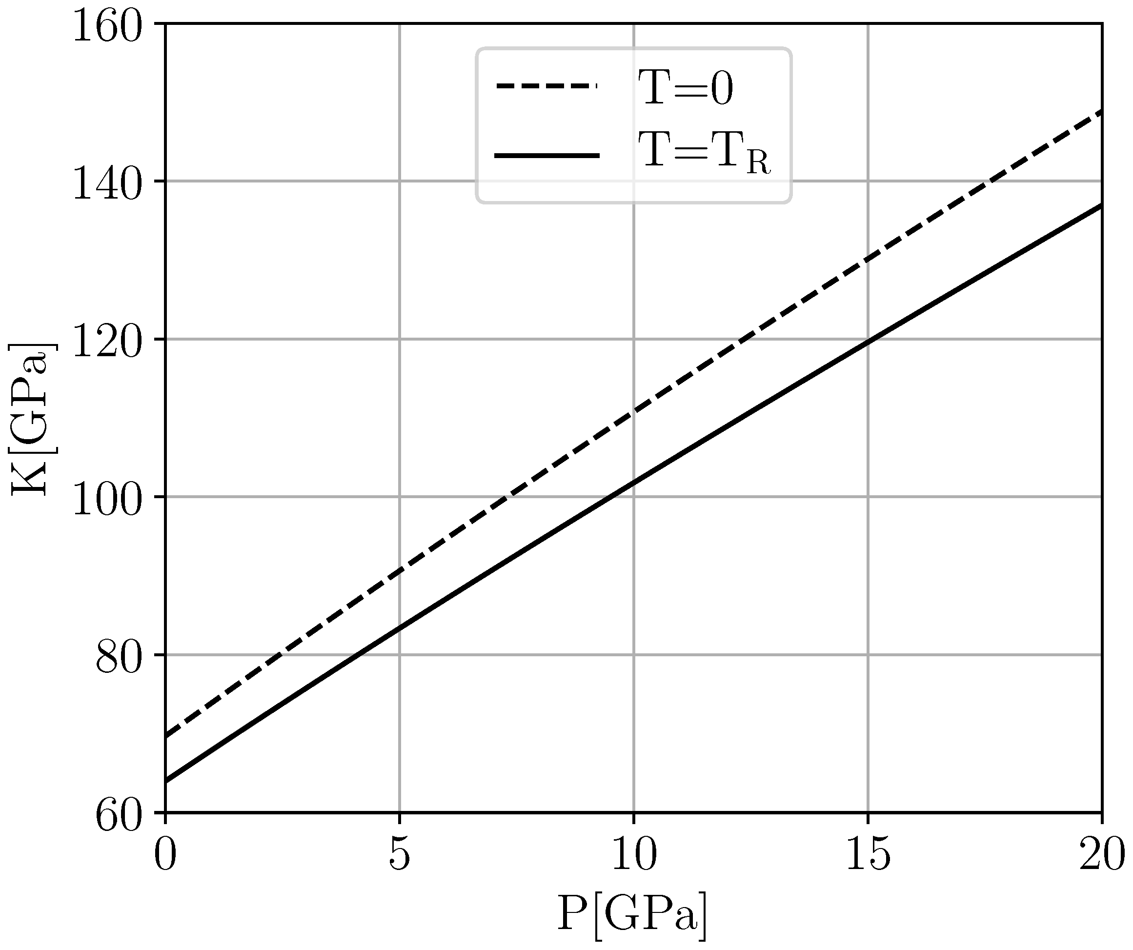
Since we do not need to maintain the highest possible precision in determining
at room temperature but can content ourselves with a reasonable approximation, we use the following heuristic strategy to promote the DFT result
from
to ambient temperature.
Figure 7 shows a comparison of the bulk moduli
calculated from DFT to the result for
obtained from the Murnaghan fit of the data published in Ref. [
11]. Numerically, one finds the fraction of these moduli stays entirely within the narrow bounds
over the whole interval
. We therefore postulate a similar behavior for
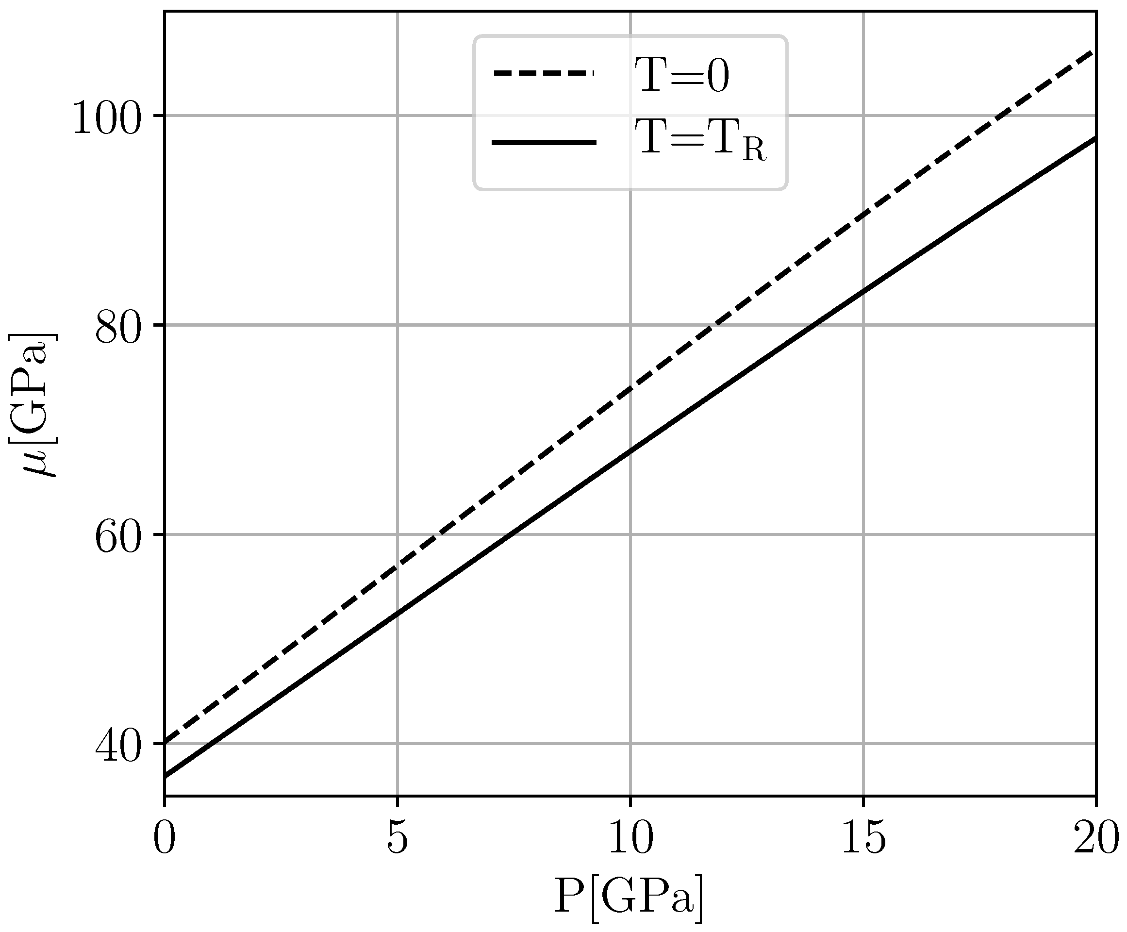
, setting
Figure 8 illustrates the resulting behavior of
.
With all other ingredients in place, this leaves only the higher order coefficients as the remaining undetermined parameters of FSLT. It therefore seems that these parameters must be treated as unknown fit parameters in a practical application. In the next section, however, we will introduce a much more convenient and powerful approach.
5. Efficient Parametrization
Comparing the above symmetry-adapted system of equations to what we had before, a considerable structural simplification is obvious. However, the following drawbacks seem to persist:
Truncating the functions defined by Equation (24b) at finite order still results in divergent behavior with increasing P.
In addition to a given set of strain measurements which we would want to feed to least squares fits based on Landau theory, rather accurate experimental information on the critical temperature or the critical pressure is frequently available from complementary experimental measurements. Unfortunately, least squares fitting procedures of strain measurements with an unconstrained value of or frequently tend to displace or and thus degrade the accuracy of the fit in the transition region. At least for a second order transition, the critical point is, of course, determined by the zero of the quadratic coefficient of the Landau expansion. Therefore, we would like to be able to explicitly constrain the behavior of , possibly fixing both its zero and/or slope at zero as a function of T or P. Unfortunately, based on a set of interrelated truncated power series, this is still hard to do.
In what follows, we propose a new scheme which finally allows for practically overcoming all of these problems in a single push. Let us start by taking a second look at
Figure 6. Of course, the correct functional form of
that we are looking for should be that of a well-behaved function passing through zero around
. At
, however, it should start out with roughly twice the initial slope of the purely linear yellow curve if we are to retain the ambient pressure Landau parameters. The pressure dependence of the correct function
must therefore be far from linear. Experimentally, there is no indication of a re-entrant behavior below
, so we do not expect any second crossing point in this pressure range. Unfortunately, our numerical tests quickly revealed that, using a truncated version of
as defined in (
29), it seems virtually impossible to meet these requirements unless one is willing to go to prohibitively high truncation order, thus introducing a plethora of unknown fit parameters and the accompanying horrific numerical problems.
A way out is to propose a reasonable function
in closed form that meets all of the above requirements while still containing some adjustable parameters that offer a certain amount of variational flexibility to allow improvement by least squares fitting. Of course, there are many ways to do this, and the choices are only limited by the reader’s ingenuity. In fact, since the summand
of
contributes the lowest order coefficient
, which is usually fixed from knowledge of an existing ambient pressure Landau theory, all candidate functions
that start out like
qualify as candidates for a meaningful function
. In our current application to KMF, we parametrize
by introducing the function
with parameters
combining a linear part with slope
c and a nonlinear contribution
, which remains yet to be specified. Our general parametrization strategy is then as follows:
As a function of e, should start out with slope , so parameter b can be traded for the slope s of at .
Suppose further that should vanish at a critical value of the background strain e. For , this implies the constraint equation where , which may be solved for parameter c.
These steps eliminate parameters
in favor of the constants
and
, leaving
d as the single remaining free variational parameter. We still need to reconcile this parametrization of
with that of the function
as defined in Equation (24b). We focus on the power series part
which is based on the same set of coefficients
as
but lacks the accompanying factorials
. These factorials can, however, easily be taken care of. Observe that
Therefore, using the
Borel transform
we may relate
It remains to specify a suitable function . Beyond producing a reasonable function , the job profile for recruiting such a function includes at least two basic requirements:
It would be highly desirable to be able to compute the corresponding Borel transform in closed form.
should also allow for solving the equation explicitly.
For the present goal of understanding the HPPT in KMF, we came up with the choice
(note that
for
) which meets both of these minimal requirements, since, in this case,
and
In this way, we have completely bypassed Taylor series expansions and their various accompanying drawbacks.
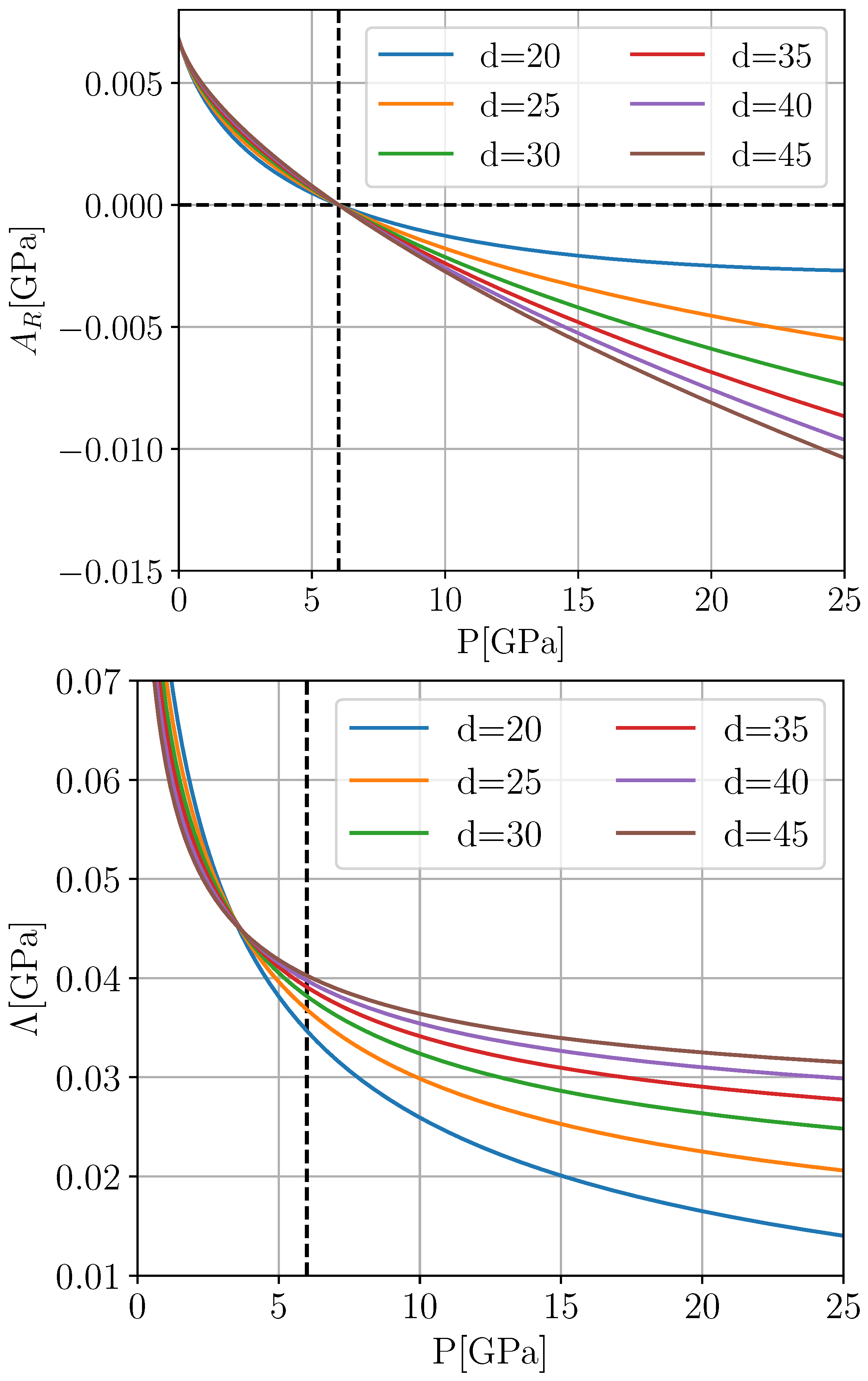
Figure 9 illustrates the remaining variational freedom in our chosen parametrization.
In summary, at this stage, the function
which governs the behavior of
and—through a Borel transform—also provides the coupling function
between the spontaneous volume strain
and
according to Equation (
25) has been specified up to a single free parameter
d. The remaining coupling function
explicitly determines the proportionality between the spontaneous tetragonal strain
and
, However, both
and
also enter implicitly into the spontaneous strain via its implicit dependence on the quartic coefficient
of the renormalized Landau potential as given by Equation (28b), and, apart from the reasonable requirement
, nothing is known in advance about its pressure dependence, such that introducing a truncated Taylor series and least squares fitting seems unavoidable. However, we can actually do a lot better than this. Let us consider experimental high pressure spontaneous strain data in the form of
n data points
. In fact, at a given prescribed pressure value
and with all other parameters in place, we can regard the room temperature values
and
as functions of the-unknown-function values
. The “best” value
matching the data point
may then be determined by numerically minimizing the function
with weights
suitable adjusted to counterbalance size differences between
and
. Carried out for all
, this prescription results in a collection of
n “optimal” values
from which one may hope to recover the full function
by interpolation.
Figure 10 shows the result of our corresponding effort for KMF. Amazingly, we observe that all values
seem to accumulate on a straight line whose extrapolation
perfectly passes through the point
, which is just the limiting value imposed by ambient pressure Landau theory. We believe that this behavior is not coincidental but a strong indication that the present parametrization is internally consistent and correct.
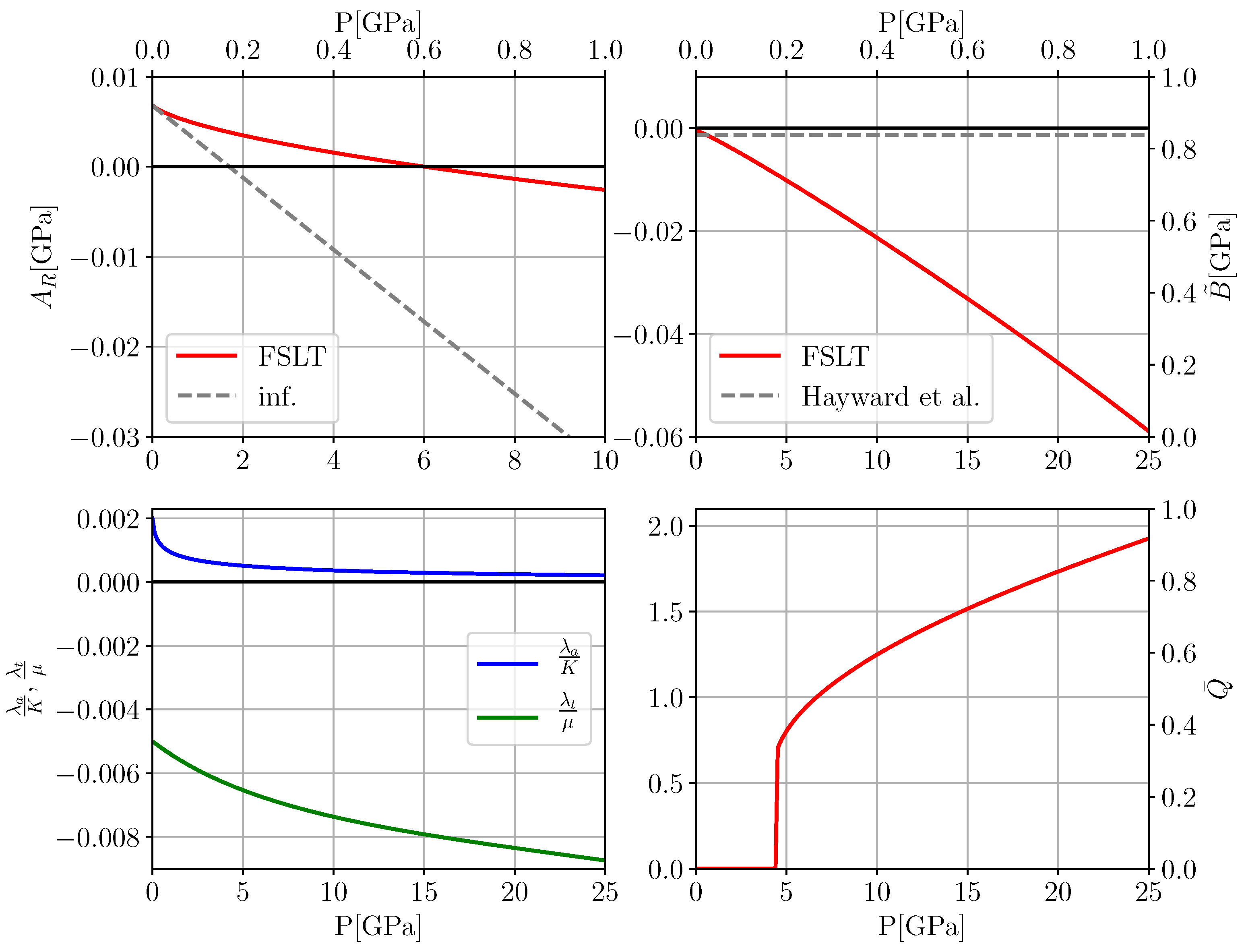
A simple linear fit of
therefore completes our Landau parametrization. Our results for the pressure dependence of the couplings
and the resulting pressure dependence of the equilibrium OP
are illustrated in
Figure 11. Note that in the present description the transition appears to be of first rather than second order, with
yielding a transition pressure
. Finally, the resulting parametrization of the spontaneous strain is compared to experiment in
Figure 12.
6. Discussion
For the high pressure community, our present paper contains some good news and some bad news—first, the bad news. We hope to have demonstrated convincingly that classical Landau theory is usually completely inadequate for “explaining” experimental findings in the field of high pressure phase transitions, and the conclusions drawn from it will often be misleading at best. Taking the example of KMF, both the first order character of the transition and the correct value of the transition pressure are completely obscured by sticking to Landau theory with infinitesimal strain coupling, even if one is willing to distort a pre-existing ambient pressure Landau parametrization beyond recognition. The good news, however, is that with the development of FSLT a mathematically consistent alternative incorporating nonlinear elasticity has recently become available. Up to now, however, FSLT has been rather complicated in structure, which quite likely scared off many potential users and thus did not lead to the widespread use that its developers were initially hoping for. The present paper, which exploits the enormous simplifications that arise by passing (i) from Cartesian to symmetry-adapted finite strains and (ii) by virtue of (i), from truncated Taylor expansions to a functional parametrization. These improvements should pave the way for routine use of our theory in successfully describing HPPTs. In particular, the present paper illustrates that, while the former version of FSLT involved delicate least-squares fitting procedures with a large number of unknown fit parameters and dealing with all the inadequacies implicit in the use of truncated Taylor expansions, in the present scheme, the unknown pressure dependencies can be systematically determined one-by-one in a step-wise, almost “deterministic” manner.
Admittedly, even the present parametrization of the HPPT in KMF is still less than perfect. For instance, the coupling function
shown in the lower left panel of
Figure 11 exhibits a steep initial decrease with increasing pressure. Since no spontaneous strain data are available for this pressure region, this does not change the physical values produced by the theory. However, it hints at a sub-optimal choice Equation (
38) for the auxiliary function
. The reader is invited to come up with an improved candidate function.
More importantly, in a full-blown application of FSLT, we should be able to predict e.g., the
cubic-to-tetragonal phase boundary of KMF and compute pressure—and temperature-dependent elastic constants. In principle, the ability to do so depends mainly on the successful construction of a pressure—and temperature-dependent baseline, i.e., the cubic EOS
. In a previous paper [
10], this task has been successfully carried out for the perovskite
by combining zero temperature DFT calculations (see
Appendix A for details) with the Debye approximation as implemented in the
Gibbs2 package [
22,
23] to incorporate effects of thermal expansion (recently, we learned [
24] that a similar approach also seems to work for
). Unfortunately, our corresponding efforts to derive
for KMF along the same lines have failed so far, however. This failure manifests itself e.g., in the inability to simultaneously reproduce the thermal baseline at
measured experimentally and the ambient temperature EOS, even if we allowed for the introduction of a constant compensating background pressure which is frequently introduced in DFT calculations to compensate inadequacies of an employed exchange-correlation functional. Ref. [
25] states that perovskites with octahedral tilting generally do not show an appreciable coupling between structural and magnetic order parameters. Nevertheless, this statement obviously does not exclude effects due to a coupling between magnetic degrees of freedom and the background volume strain. Since the Debye approximation is based exclusively on phonons, we may speculate that in KMF residual magnetic effects may be responsible for additional thermal energy consumption. An investigation of this problem is currently underway.
Finally, it may be argued that our current theory also does not “explain” the origins of the involved nonlinear
P-dependencies on a fundamental level. In approaches based on infinitesimal strain couplings, similarly looking
P-dependent couplings are also introduced, but in a more or less completely ad hoc manner, blaming their existence on rather unspecific “higher order strain couplings”. As a rule, such an approach results in a mathematically inconsistent theory. In contrast, the nonlinearities that arise in FSLT result for different but well-defined reasons. On the one hand, there are couplings between powers of the background strain
and the Landau potential
“floating” on this background strain, and there is a pressure-dependence of the elastic moduli
and
, which is in principle accessible e.g., to DFT calculations. This leaves the task of “explaining” the residual nonlinearities in the functions
describing the couplings between order parameter and spontaneous strains. In contrast to blaming their existence on the effects of some unspecified higher order couplings, our present theory provides a practical way to numerically determine these functions. In addition, we see no reason in principle as to why such
P-dependent coupling constants could not eventually be extracted from DFT calculations along the general philosophy laid out in Refs. [
26,
27] and the subsequent follow-up literature.


