Mueller Matrix Polarimetric Imaging Analysis of Optical Components for the Generation of Cylindrical Vector Beams

 , , , and
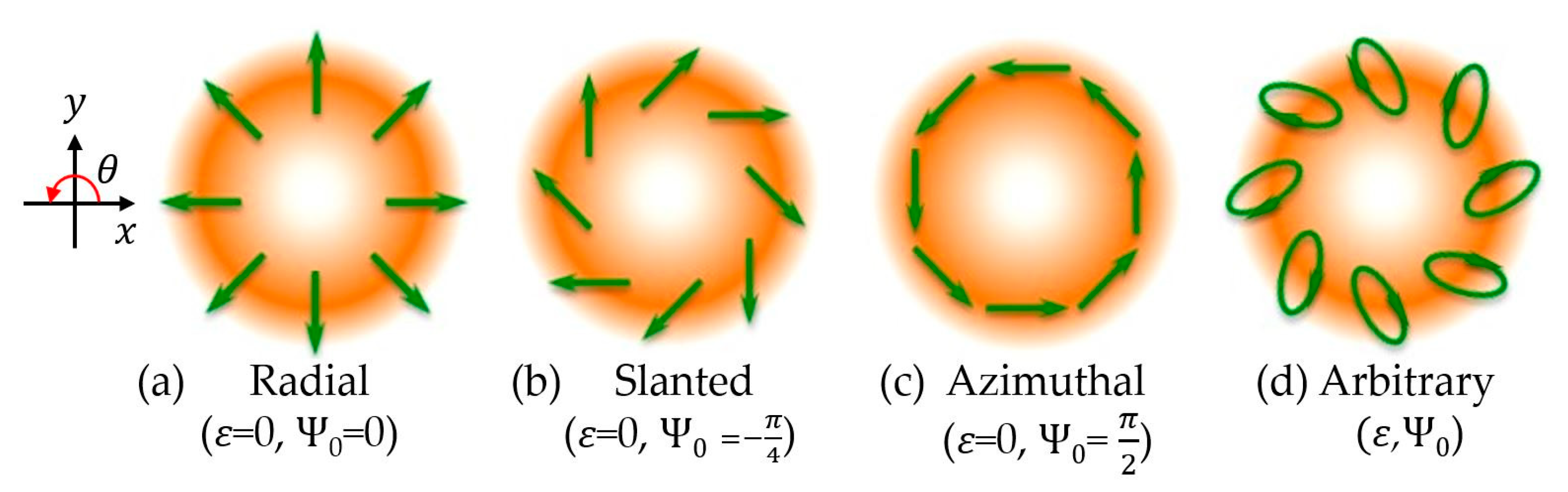
Abstract
1. Introduction
2. Materials and Methods
2.1. Vector Beams in the Stokes formalism
2.2. Mueller Matrix of an Ideal Radial Polarizer and an Ideal Q-Plate
2.2.1. Radial Polarizer
2.2.2. Q-Plates
2.3. Mueller Matrix Decomposition
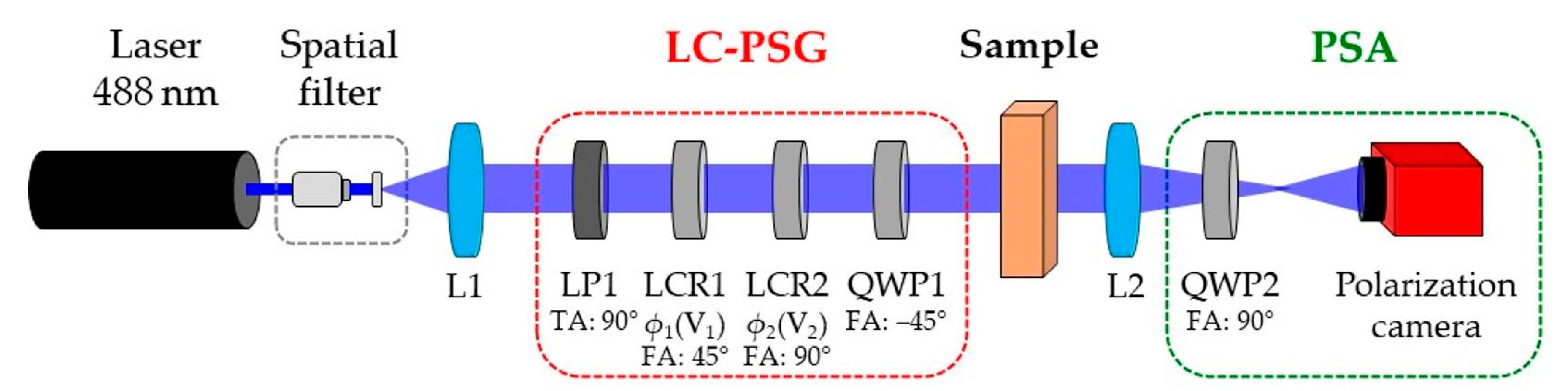
3. Experimental Arrangement of the Mueller Matrix Polarimeter
4. Results and Discussion
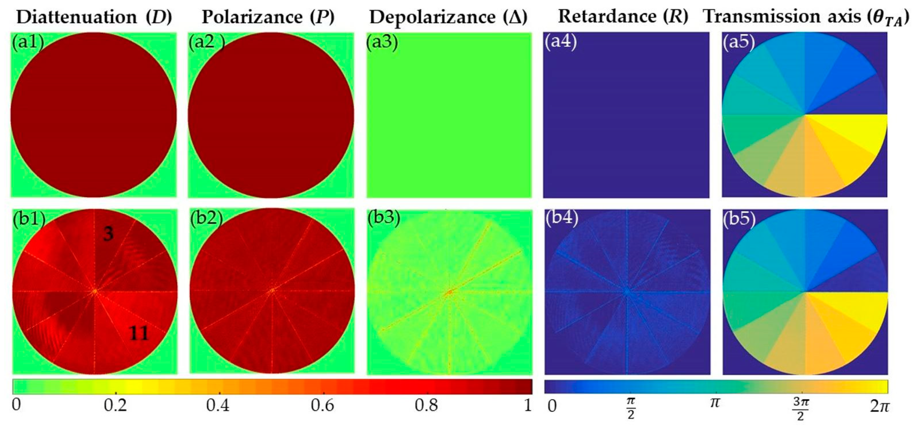
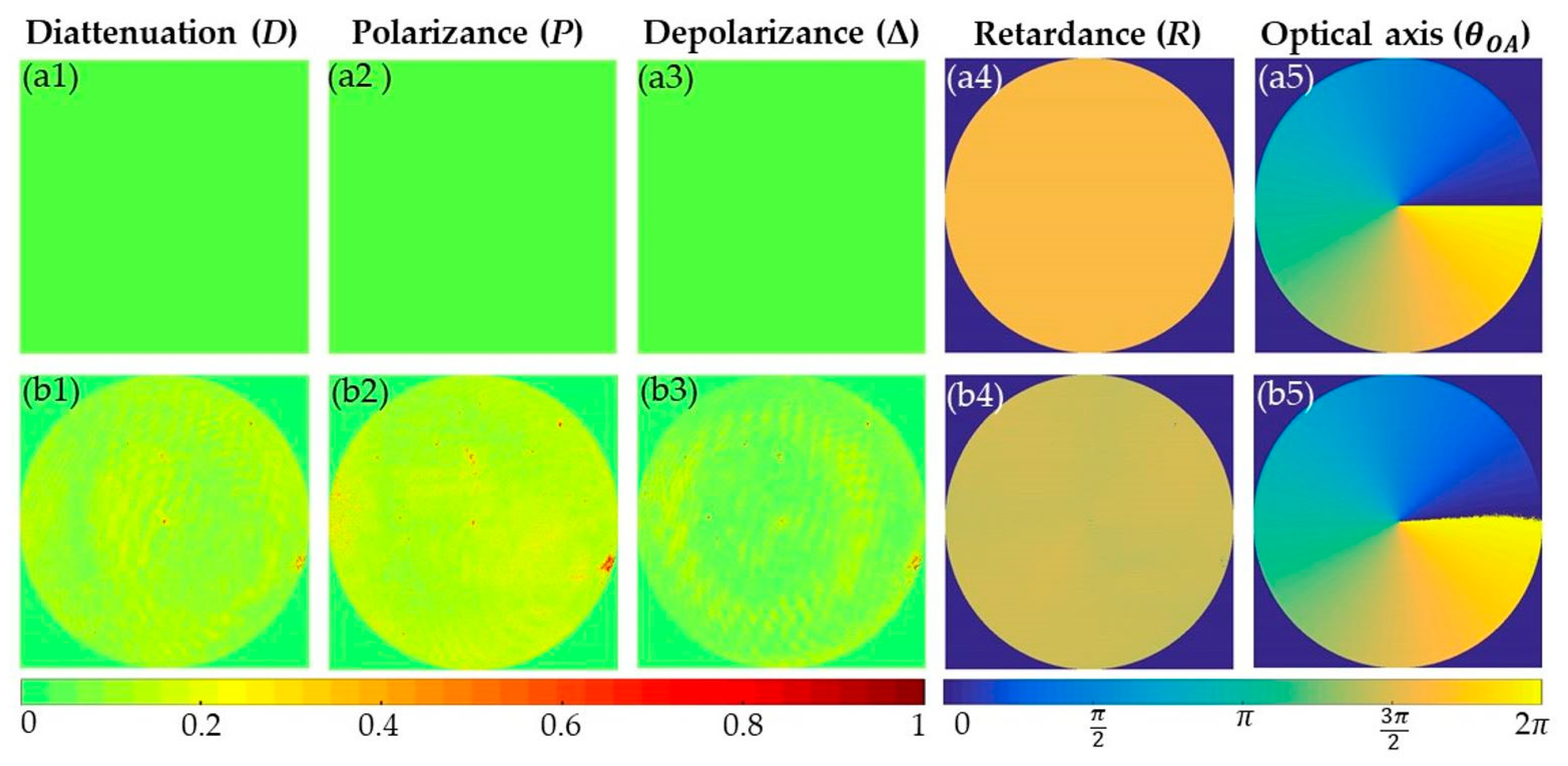
4.1. Imaging Mueller Matrix Results of the Radial Polarizer
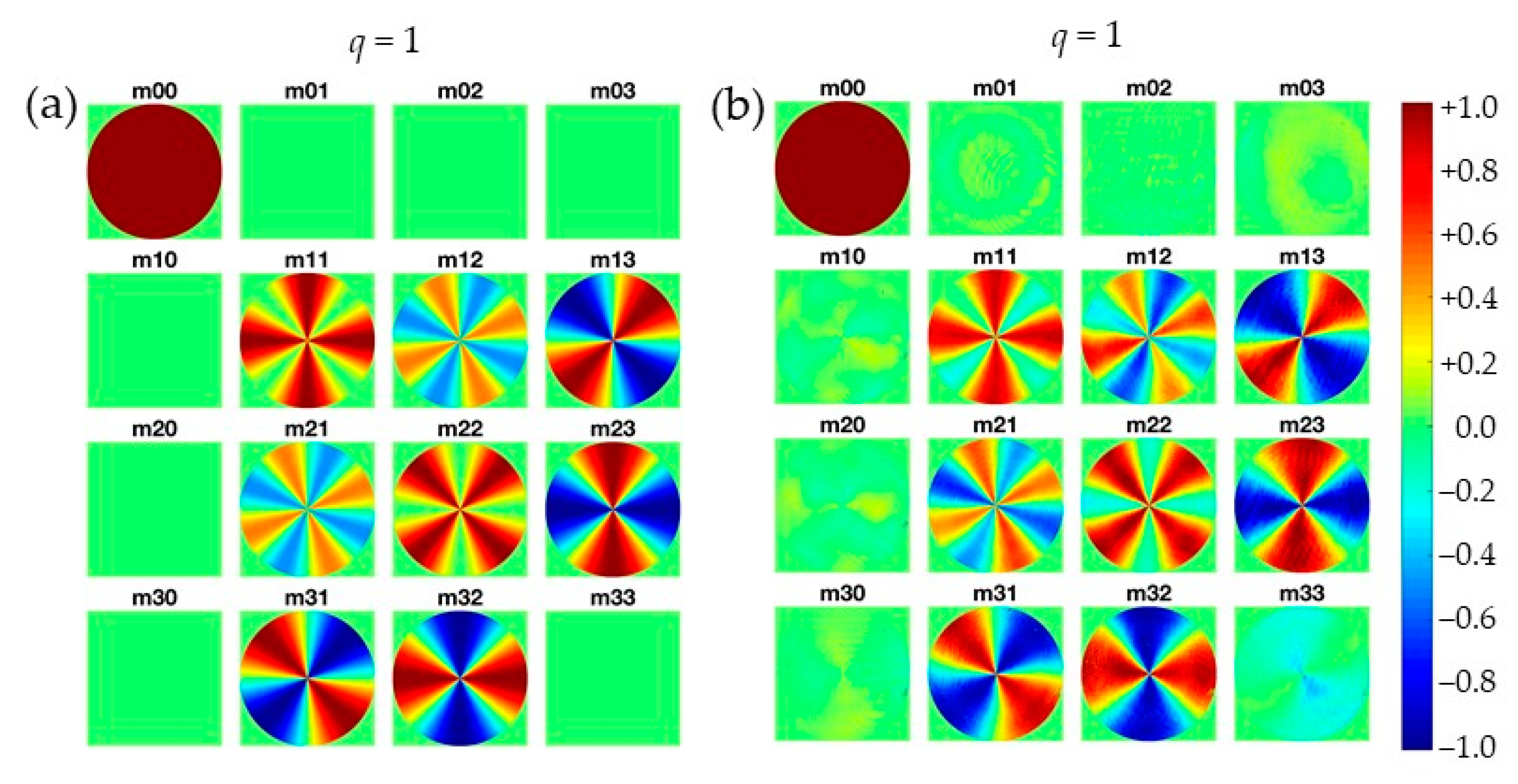
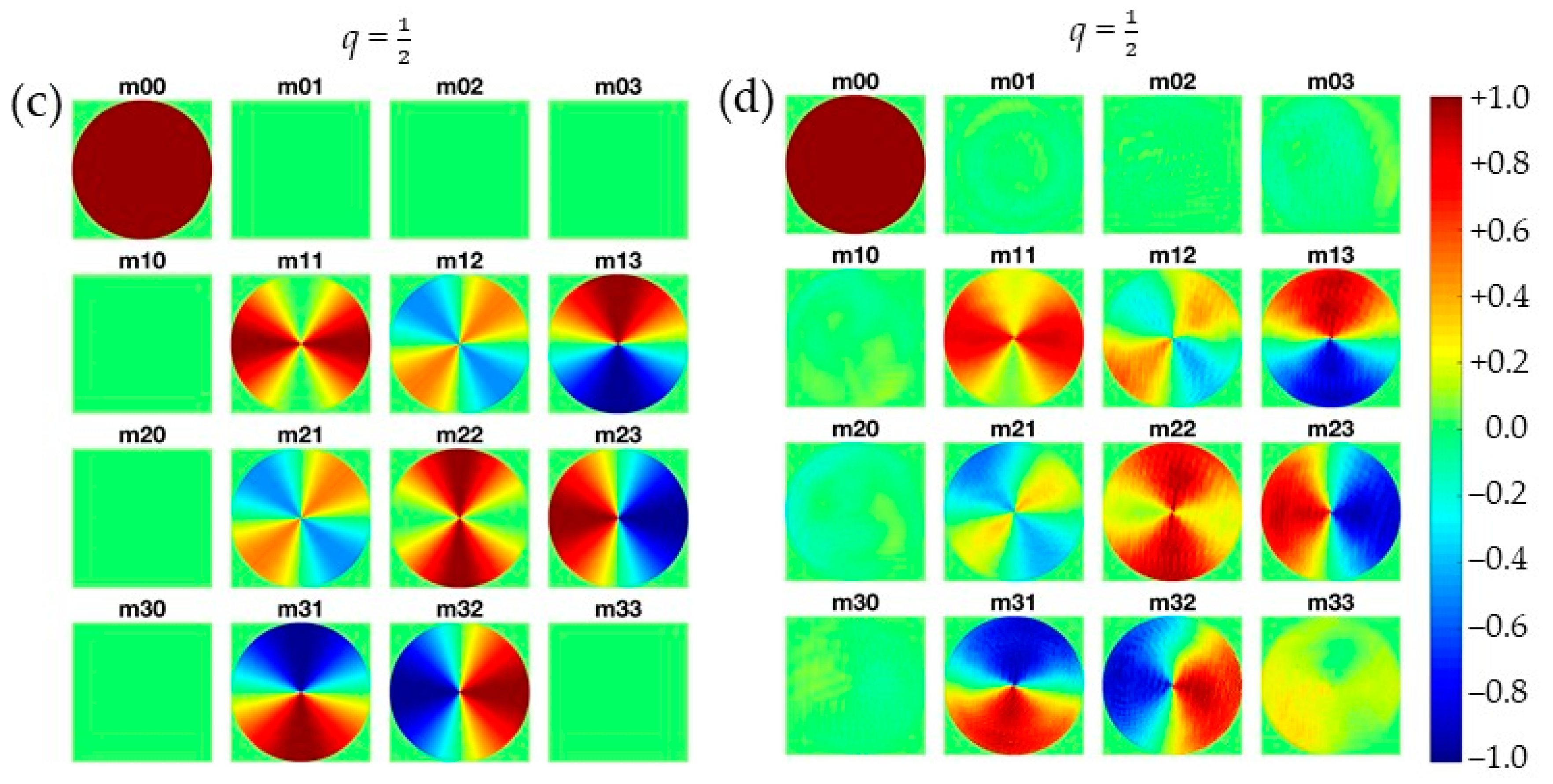
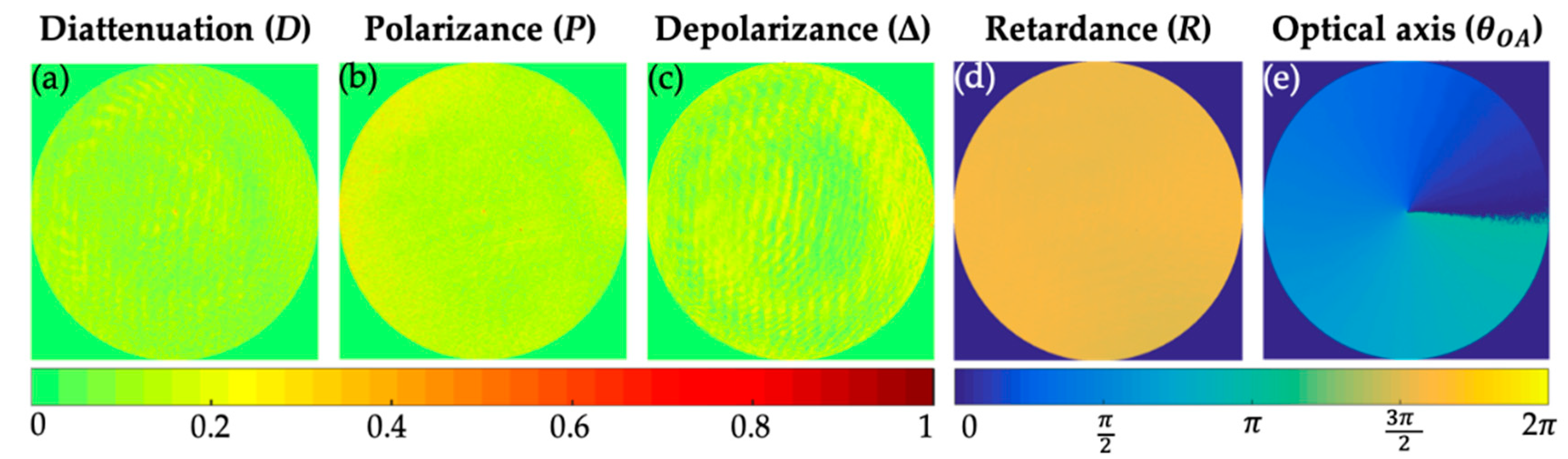
4.2. Imaging Mueller Matrix Results of the q-Plate
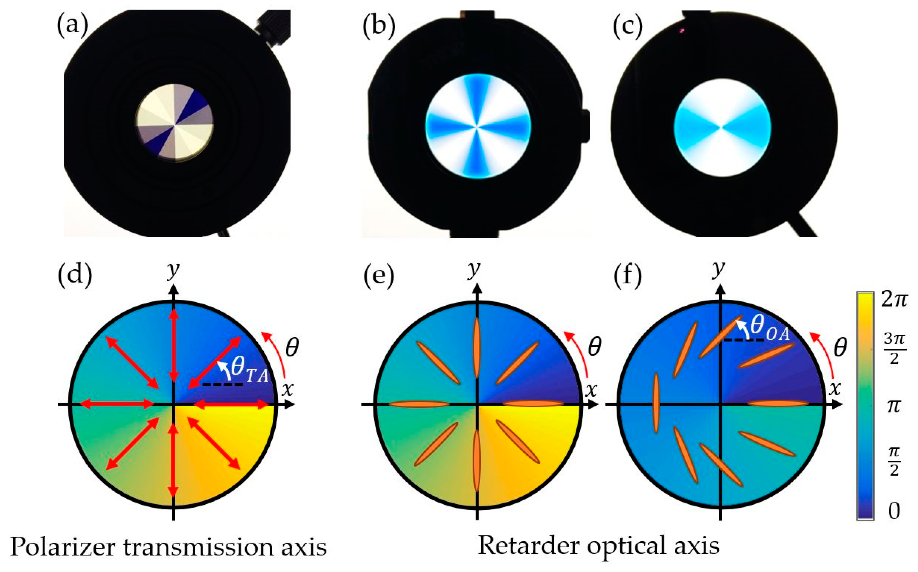
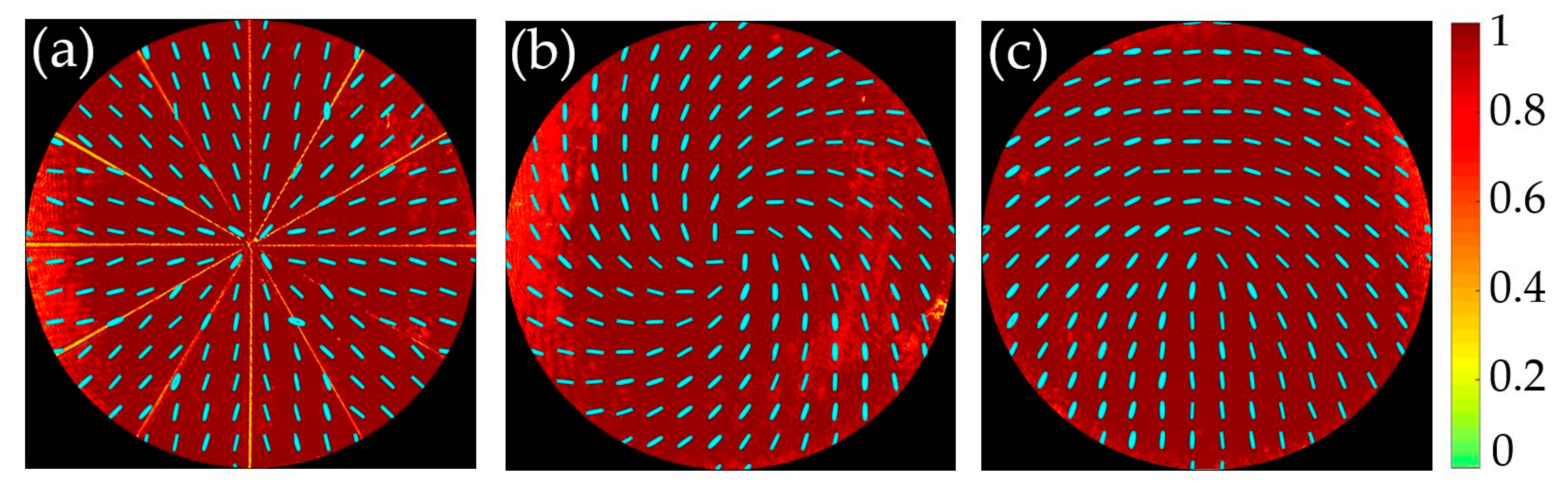
4.3. Polarization Map of the CVBs Generated by the Radial Polarizer and the q-Plates
5. Conclusions
Author Contributions
Funding
Conflicts of Interest
Appendix A
Appendix A.1. Case of a Singular Diattenuation Matrix
Appendix A.2. Case of a Non-Singular Diattenuation Matrix
References
- Beeckman, J.; Neyts, K.; Vanbrabant, P.J.M. Liquid-crystal photonic applications. Opt. Eng. 2011, 50, 081202. [Google Scholar] [CrossRef]
- Bueno, J.M. Polarimetry using liquid-crystal variable retarders: Theory and calibration. J. Opt. A Pure Appl. Opt. 2000, 2, 216–222. [Google Scholar] [CrossRef]
- Uribe-Patarroyo, N.; Alvarez-Herrero, A.; Heredero, R.L.; Iniesta, J.C.D.T.; Jiménez, A.C.L.; Domingo, V.; Gasent, J.L.; Jochum, L.; Pillet, V.M. IMaX: A polarimeter based on Liquid Crystal Variable Retarders for an aerospace mission. Phys. Status Solidi 2008, 5, 1041–1045. [Google Scholar] [CrossRef]
- Tyo, J.S.; Goldstein, D.L.; Chenault, D.B.; Shaw, J.A. Review of passive imaging polarimetry for remote sensing applications. Appl. Opt. 2006, 45, 5453–5469. [Google Scholar] [CrossRef] [PubMed]
- Lizana, A.; Foldyna, M.; Stchakovsky, M.; Georges, B.; Nicolas, D.; Garcia-Caurel, E. Enhanced sensitivity to dielectric function and thickness of absorbing thin films by combining total internal reflection ellipsometry with standard ellipsometry and reflectometry. J. Phys. D Appl. Phys. 2013, 46, 105501. [Google Scholar] [CrossRef]
- Lizana, A.; Van Eeckhout, A.; Adamczyk, K.; Rodríguez, C.; Escalera, J.C.; Garcia-Caurel, E.; Moreno, I.; Campos, J. Polarization gating based on Mueller matrices. J. Biomed. Opt. 2017, 22, 056004. [Google Scholar] [CrossRef]
- Bueno, J.M.; Hunter, J.J.; Cookson, C.J.; Kisilak, M.L.; Campbell, M.C.W. Improved scanning laser fundus imaging using polarimetry. J. Opt. Soc. Am. A 2007, 24, 1337–1348. [Google Scholar] [CrossRef]
- Wolfe, J.E.; Chipman, R.A. Polarimetric characterization of liquid-crystal-on-silicon panels. Appl. Opt. 2006, 45, 1688–1703. [Google Scholar] [CrossRef]
- Lizana, A.; Moreno, I.; Iemmi, C.; Márquez, A.; Campos, J.; Yzuel, M. Time-resolved Mueller matrix analysis of a liquid crystal on silicon display. Appl. Opt. 2008, 47, 4267–4274. [Google Scholar] [CrossRef]
- Ding, Z.; Yao, Y.; Yao, X.S.; Chen, X.; Wang, C.; Wang, S.; Liu, T. Demonstration of Compact In situ Mueller-Matrix Polarimetry Based on Binary Polarization Rotators. IEEE Access 2019, 7, 144561–144571. [Google Scholar] [CrossRef]
- Parejo, P.G.; Campos-Jara, A.; Garcia-Caurel, E.; Arteaga, O.; Alvarez-Herrero, A. Nonideal optical response of liquid crystal variable retarders and its impact on their performance as polarization modulators. J. Vac. Sci. Technol. B 2020, 38, 014009. [Google Scholar] [CrossRef]
- Marc, P.; Bennis, N.; Spadlo, A.; Kalbarczyk, A.; Węgłowski, R.; Garbat, K.; Jaroszewicz, L.R. Monochromatic Depolarizer Based on Liquid Crystal. Crystals 2019, 9, 387. [Google Scholar] [CrossRef]
- Rosales-Guzmán, C.; Ndagano, B.; Forbes, A. A review of complex vector light fields and their applications. J. Opt. 2018, 20, 123001. [Google Scholar] [CrossRef]
- Zhan, Q. Cylindrical vector beams: From mathematical concepts to applications. Adv. Opt. Photonics 2009, 1, 1–57. [Google Scholar] [CrossRef]
- Pachava, S.; Dharmavarapu, R.; Anand, V.; Jayakumar, S.; Manthalkar, A.; Dixit, A.; Viswanathan, N.K.; Srinivasan, B.; Bhattacharya, S. Generation and decomposition of scalar and vector modes carrying orbital angular momentum: A review. Opt. Eng. 2019, 59, 041205. [Google Scholar] [CrossRef]
- De Sande, J.C.G.; De Sande, J.C.G.; Santarsiero, M.; Piquero, G. Mueller matrix polarimetry using full Poincaré beams. Opt. Lasers Eng. 2019, 122, 134–141. [Google Scholar] [CrossRef]
- Zhao, B.; Hu, X.-B.; Rodriguez-Fajardo, V.; Zhu, Z.-H.; Gao, W.; Forbes, A.; Rosales-Guzmán, C. Real-time Stokes polarimetry using a digital micromirror device. Opt. Express 2019, 27, 31087–31093. [Google Scholar] [CrossRef]
- Stalder, M.; Schadt, M. Linearly polarized light with axial symmetry generated by liquid-crystal polarization converters. Opt. Lett. 1996, 21, 1948–1950. [Google Scholar] [CrossRef]
- Rubano, A.; Cardano, F.; Piccirillo, B.; Marrucci, L. Q-plate technology: A progress review. J. Opt. Soc. Am. B 2019, 36, D70–D87. [Google Scholar] [CrossRef]
- Cardano, F.; Karimi, E.; Slussarenko, S.; Marrucci, L.; De Lisio, C.; Santamato, E. Polarization pattern of vector vortex beams generated by q-plates with different topological charges. Appl. Opt. 2012, 51, C1–C6. [Google Scholar] [CrossRef]
- Nersisyan, S.; Tabiryan, N.; Steeves, D.M.; Kimball, B.R. Fabrication of liquid crystal polymer axial waveplates for UV-IR wavelengths. Opt. Express 2009, 17, 11926–11934. [Google Scholar] [CrossRef] [PubMed]
- Beresna, M.; Gecevičius, M.; Kazansky, P.G.; Gertus, T. Radially polarized optical vortex converter created by femtosecond laser nanostructuring of glass. Appl. Phys. Lett. 2011, 98, 201101. [Google Scholar] [CrossRef]
- Sánchez-López, M.M.; Moreno, I.; Davis, J.A.; Puerto-Garcia, D.; Abella, I.; Delaney, S.W. Extending the use of commercial q-plates for the generation of high-order and hybrid vector beams. Laser Beam Shap. XVIII 2018, 10744, 1074407. [Google Scholar] [CrossRef]
- Badham, K.; Delaney, S.; Hashimotono, N.; Sánchez-López, M.M.; Kurihara, M.; Tanabe, A.; Moreno, I.; Davis, J.A. Generation of vector beams at 1550 nm telecommunications wavelength using a segmented q -plate. Opt. Eng. 2016, 55, 30502. [Google Scholar] [CrossRef]
- Quiceno-Moreno, J.C.; Marco, D.; Sánchez-López, M.M.; Solarte, E.; Moreno, I. Analysis of Hybrid Vector Beams Generated with a Detuned Q-Plate. Appl. Sci. 2020, 10, 3427. [Google Scholar] [CrossRef]
- Moreno, I.; Albero, J.; Davis, J.A.; Cottrell, D.M.; Cushing, J.B. Polarization manipulation of radially polarized beams. Opt. Eng. 2012, 51, 128003. [Google Scholar] [CrossRef]
- Lu, S.-Y.; Chipman, R.A. Interpretation of Mueller matrices based on polar decomposition. J. Opt. Soc. Am. A 1996, 13, 1106–1113. [Google Scholar] [CrossRef]
- Morales, G.L.; Sánchez-López, M.D.M.; Soriano, I.M. Liquid-crystal polarization state generator. In Proceedings of the Unconventional Optical Imaging II, Online. Strasbourg, France, 7–10 April 2020; p. 11351. [Google Scholar] [CrossRef]
- Goldstein, D.H. Polarized Light; Marcel Dekker: New York, NY, USA, 2010. [Google Scholar]
- CODIXX. Available online: https://www.codixx.de/en/colorpol-s-patterned/colorpol-s-patterned-polarizer.html (accessed on 2 November 2020).
- THORLABS. Available online: https://www.thorlabs.com/newgrouppage9.cfm?objectgroup_id=9098 (accessed on 2 November 2020).
- Marco, D.; Sánchez-López, M.M.; García-Martínez, P.; Moreno, I. Using birefringence colors to evaluate a tunable liquid-crystal q-plate. J. Opt. Soc. Am. B 2019, 36, D34–D41. [Google Scholar] [CrossRef]
- Sánchez-López, M.M.; Abella, I.; Puerto-García, D.; Davis, J.A.; Moreno, I. Spectral performance of a zero-order liquid-crystal polymer commercial q-plate for the generation of vector beams at different wavelengths. Opt. Laser Technol. 2018, 106, 168–176. [Google Scholar] [CrossRef]
- Morio, J.; Goudail, F. Influence of the order of diattenuator, retarder, and polarizer in polar decomposition of Mueller matrices. Opt. Lett. 2004, 29, 2234–2236. [Google Scholar] [CrossRef]
- Ossikovski, R.; De Martino, A.; Guyot, S. Forward and reverse product decompositions of depolarizing Mueller matrices. Opt. Lett. 2007, 32, 689–691. [Google Scholar] [CrossRef] [PubMed]
- ArcOptix. Variable Phase Retarder. Available online: http://www.arcoptix.com/variable_phase_retarder.htm (accessed on 2 November 2020).
- Hinds Instruments. Mueller Polarimeters. Available online: https://www.hindsinstruments.com/products/polarimeters/mueller-polarimeter/ (accessed on 4 December 2020).
- Espinosa-Luna, R.; Zhan, Q. Polarization and Polarizing Optical Devices. In Fundamentals and Basic Optical Instruments, Handbook of Optical Engineering; CRC Press: New York, NY, USA, 2017. [Google Scholar]
- Vargas, J.; Uribe-Patarroyo, N.; Quiroga, J.A.; Alvarez-Herrero, A.; Belenguer, T. Optical inspection of liquid crystal variable retarder inhomogeneities. Appl. Opt. 2010, 49, 568–574. [Google Scholar] [CrossRef] [PubMed]
- Moallemi, P.; Behnampourii, M. Adaptive optimum notch filter for periodic noise reduction in digital images. AUT J. Electr. Eng. 2010, 42, 1–7. [Google Scholar]
- Smith, M.H.; Woodruff, J.B.; Howe, J.D. Beam wander considerations in imaging polarimetry. In Proceedings of the SPIE’s International Symposium on Optical Science, Engineering, and Instrumentation, Denver, CO, USA, 18–23 July 1999; Volume 3754, pp. 50–54. [Google Scholar] [CrossRef]
- Gil, J.J.; Ossikovski, R. Polarized Light and the Mueller Matrix Approach; CRC Press: Boca Raton, FL, USA, 2016. [Google Scholar]
- Ju, H.; Ren, L.; Liang, J.; Qu, E.; Bai, Z. Method for Mueller matrix acquisition based on a division-of-aperture simultaneous polarimetric imaging technique. J. Quant. Spectrosc. Radiat. Transf. 2019, 225, 39–44. [Google Scholar] [CrossRef]
- Ji, W.; Lee, C.-H.; Chen, P.; Hu, W.; Ming, Y.; Zhang, L.; Lin, T.-H.; Chigrinov, V.G.; Lu, Y.-Q. Meta-q-plate for complex beam shaping. Sci. Rep. 2016, 6, 25528. [Google Scholar] [CrossRef]
- Rafayelyan, M.; Brasselet, E. Laguerre–Gaussian modal q-plates. Opt. Lett. 2017, 42, 1966–1969. [Google Scholar] [CrossRef]
- Holland, J.E.; Moreno, I.; Davis, J.A.; Sánchez-López, M.M.; Cottrell, D.M. Q-plates with a nonlinear azimuthal distribution of the principal axis: Application to encoding binary data. Appl. Opt. 2018, 57, 1005–1010. [Google Scholar] [CrossRef]


Publisher’s Note: MDPI stays neutral with regard to jurisdictional claims in published maps and institutional affiliations. |
© 2020 by the authors. Licensee MDPI, Basel, Switzerland. This article is an open access article distributed under the terms and conditions of the Creative Commons Attribution (CC BY) license (http://creativecommons.org/licenses/by/4.0/).
Share and Cite
López-Morales, G.; Sánchez-López, M.d.M.; Lizana, Á.; Moreno, I.; Campos, J. Mueller Matrix Polarimetric Imaging Analysis of Optical Components for the Generation of Cylindrical Vector Beams. Crystals 2020, 10, 1155. https://doi.org/10.3390/cryst10121155
López-Morales G, Sánchez-López MdM, Lizana Á, Moreno I, Campos J. Mueller Matrix Polarimetric Imaging Analysis of Optical Components for the Generation of Cylindrical Vector Beams. Crystals. 2020; 10(12):1155. https://doi.org/10.3390/cryst10121155
Chicago/Turabian StyleLópez-Morales, Guadalupe, María del Mar Sánchez-López, Ángel Lizana, Ignacio Moreno, and Juan Campos. 2020. "Mueller Matrix Polarimetric Imaging Analysis of Optical Components for the Generation of Cylindrical Vector Beams" Crystals 10, no. 12: 1155. https://doi.org/10.3390/cryst10121155
APA StyleLópez-Morales, G., Sánchez-López, M. d. M., Lizana, Á., Moreno, I., & Campos, J. (2020). Mueller Matrix Polarimetric Imaging Analysis of Optical Components for the Generation of Cylindrical Vector Beams. Crystals, 10(12), 1155. https://doi.org/10.3390/cryst10121155