
A Novel Approach for Prediction of Industrial Catalyst Deactivation Using Soft Sensor Modeling

Abstract
:1. Introduction
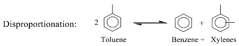
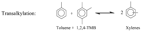
2. Kinetic Model
3. Identification Methodology
3.1. State Dependent Parameter (SDP) Model
- Reaction specific rate is a function of temperature according to the Arrhenius equation;
- Due to reversible reactions, the concentration of the reaction components is considered by a power law expression (since all the adsorption terms are included in the deactivation term); and
- Catalyst deactivation is a function of time and the concentrations of some other components. This function is assumed to be exponential (see Table 1).
3.2. Time-Varying Parameter (TVP) Estimation
3.3. Backward Pass Smoothing Equations
3.4. Back-Fitting Algorithm for SDP Models
- Assume FIS estimation has yielded prior TVP estimates of the SDPs.
- Iterate:
- Form the MDV: .
- Sort both and according to the ascending order of .
- Obtain an FIS estimate of in the MDV relationship .
- Repeat steps 2–5 until convergence criterion occurs.
4. Results and Discussion
- Modeling is based on the continuity equation;
- Grey-box model is considered;
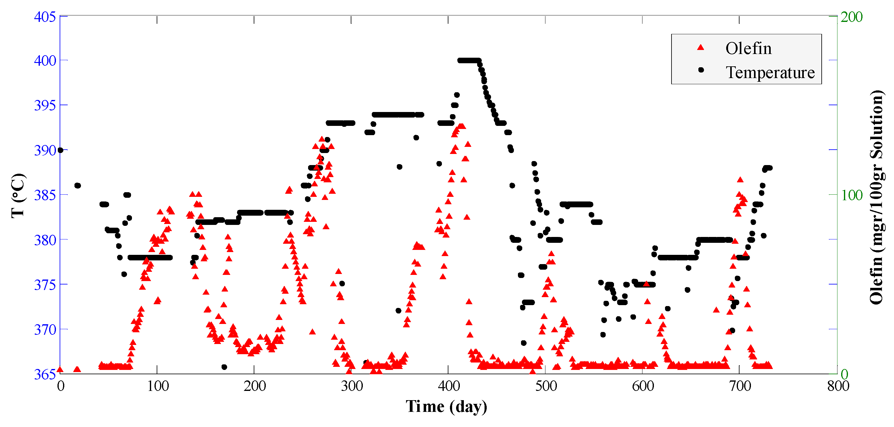
- Data are registered as daily average, that is, for each 24 h one data is recorded;
- Since the residence time of the reactor is half an hour and the data are recorded per day, the system is considered stable and the term for the accumulation in the continuity equation is vanishes;
- Due to the high volumetric flow rate of the reactor, the terms for the axial and radial diffusions are considered as part of the system error and hence removed; and
- The hydrogen molar percentage in the feed is about 90%. Therefore, the internal porous mass transfer resistance is disregarded.
5. Conclusions
Acknowledgment
Author Contributions
Conflicts of Interest
Symbols
| the term of catalyst deactivation based on the DP reaction (h−1) | |
| the term of catalyst deactivation based on the TA reaction (h−1) | |
| the ith coefficient of model output (–) | |
| the ith coefficient of model input (–) | |
| Ci | concentration of species in the fixed-bed reactor (kmolm−3) |
| DA | axial diffusion (m2 h−1) |
| DR | radial diffusion (m2 h−1) |
| Ei | activation energy of ith reaction(J kmol−1K−1) |
| et | observation error (–) |
| system coefficient matrix (–) | |
| the ith SDP’s coefficient matrix (–) | |
| input coefficient matrix (–) | |
| the ith SDP’s coefficient matrix (–) | |
| SDP’s coefficient matrix (–) | |
| identity matrix (–) | |
| k0i | pre-exponential factor for the ith reaction (kg·hkmol−1) |
| L | length of reactor bed (m) |
| lagrange multiplier in FIS smoothing (–) | |
| Lc | concentrated likelihood function (–) |
| N | Number of data points in time series (–) |
| number of state that the ith SDP is a function of them (–) | |
| Pi | partial pressure (Pa) |
| p | number of parameters (–) |
| the ith state dependent parameter (–) | |
| vector of model parameters (–) | |
| the error covariance matrix (–) | |
| Q | volumetric flow rate (m3 h−1) |
| covariance matrix (–) | |
| noise variance ratio matrix (–) | |
| R | gas constant (J mol−1K−1) |
| rate of generation or disappearance of component i (molkgcat.−1·h−1) | |
| r | radius of reactor bed (m) |
| S | cross-sectional area of reactor bed |
| T | temperature (K) |
| t | time (h) |
| ut | inputs (–) |
| WHSV | weight hourly space velocity (h−1) |
| state vector (–) | |
| yt | output (–) |
| Vector of outputs (–) | |
| vector of regressors (–) |
Greek Letters
| vector of parameters’ noise (–) | |
| λi | order of component in the DP reaction (–) |
| µi | order of component in the TA reaction (–) |
| error of model (–) | |
| catalyst density in the bed(kgm−3) | |
| variance of error (–) | |
| catalytic deactivation term multiplied by the pre-exponential factor (–) |
References
- Waziri, S.M.; Aitani, A.M.; Al-Khattaf, S. Transformation of Toluene and 1,2,4-Trimethylbenzene over ZSM-5 and Mordenite Catalysts: A Comprehensive Kinetic Model with Reversibility. Ind. Eng. Chem. Res. 2010, 49, 6376–6387. [Google Scholar] [CrossRef]
- Al-Khattaf, S. Catalytic transformation of toluene over a high-acidity Y-zeolite based catalyst. Energy Fuels 2006, 20, 946–954. [Google Scholar] [CrossRef]
- Wang, T.; Tsai, C.; Huang, S.T. Disproportionation of toluene and of trimethylbenzene and their transalkylation over zeolite beta. Ind. Eng. Chem. Res. 1990, 29, 2005–2012. [Google Scholar] [CrossRef]
- Tsai, T.-C.; Liu, S.-B.; Wang, I. Disproportionation and transalkylation of alkylbenzenes over zeolite catalysts. Appl. Catal. A 1999, 181, 355–398. [Google Scholar] [CrossRef]
- Tsai, T.C.; Chenb, W.H.; Lai, C.S.; Liub, S.B.; Wangc, I.; Ku, C.S. Kinetics of Toluene Disproportionation over Fresh and Coked H-mordenite. Catal. Today 2004, 97, 297–302. [Google Scholar] [CrossRef]
- Bhavlkattl, S.S.; Patwardhan, S.R. Toluene Disproportionation over Nickel-Loaded Aluminum-Deficient Mordenite 2. Kinetics. Ind. Eng. Chem. Prod. Res. Dev. 1981, 20, 106–109. [Google Scholar]
- Al-Khattaf, S.; Rabiu, S.; Tukur, N.; Alnaizy, R. Kinetics of toluene methylation over USY-zeolite catalyst in a riser simulator. Chem. Eng. J. 2008, 139, 622–630. [Google Scholar] [CrossRef]
- De Jong, K.; Mesters, C.; Peferoen, D.; Van Brugge, P.; De Groot, C. Paraffin alkylation using zeolite catalysts in a slurry reactor: Chemical engineering principles to extend catalyst lifetime. Chem. Eng. Sci. 1996, 51, 2053–2060. [Google Scholar] [CrossRef]
- Taylor, R.J.; Sherwood, D.E. Effects of process parameters on isobutane/2-butene alkylation using a solid acid catalyst. Appl. Catal. A 1997, 155, 195–215. [Google Scholar] [CrossRef]
- Sahebdelfar, S.; Kazemeini, M.; Khorasheh, F.; Badakhshan, A. Deactivation behavior of the catalyst in solid acid catalyzed alkylation: Effect of pore mouth plugging. Chem. Eng. Sci. 2002, 57, 3611–3620. [Google Scholar] [CrossRef]
- Simpson, M.F.; Wei, J.; Sundaresan, S. Kinetic analysis of isobutane/butene alkylation over ultrastable HY zeolite. Ind. Eng. Chem. Res. 1996, 35, 3861–3873. [Google Scholar] [CrossRef]
- Lobao, M.W.N.; Alberton, A.L.; Melo, S.A.B.V.; Embirucu, M.; Monteiro, J.L.F.; Pinto, J.C. Kinetics of Toluene Disproportionation: Modeling and Experiments. Ind. Eng. Chem. Res. 2012, 51, 171–183. [Google Scholar] [CrossRef]
- Fortuna, L.; Graziani, S.A.; Rizzo, S.; Xibilia, M.G. Soft Sensors for Monitoring and Control of Industrial Processes; Springer: London, UK, 2007. [Google Scholar]
- Kadleca, P.; Gabrysa, B.; Strandt, S. Data-driven Soft Sensors in the process industry. Comput. Chem. Eng. 2009, 33, 795–814. [Google Scholar] [CrossRef]
- Kaneko, H.; Arakawa, M.; Funatsu, K. Development of a New Soft Sensor Method Using Independent Component Analysis and Partial Least Squares. AIChE J. 2009, 55, 87–98. [Google Scholar] [CrossRef]
- Lin, B.; Recke, B.; Schmidt, T.M.; Knudsen, J.K.H.; Jørgensen, S.B. Data-Driven Soft Sensor Design with Multiple-Rate Sampled Data: A Comparative Study. Ind. Eng. Chem. Res. 2009, 48, 5379–5387. [Google Scholar] [CrossRef]
- Liu, J.; Chen, D.-S.; Shen, J.-F. Development of Self-Validating Soft Sensors Using Fast Moving Window Partial Least Squares. Ind. Eng. Chem. Res. 2010, 49, 11530–11546. [Google Scholar] [CrossRef]
- Liu, Y.; Gao, Z.; Chen, J. Development of soft-sensors for online quality prediction of sequential-reactor-multi-grade industrial processes. Chem. Eng. Sci. 2013, 102, 602–612. [Google Scholar] [CrossRef]
- Shang, C.; Yang, F.; Huang, D.; Lyu, W. Data-driven soft sensor development based on deep learning technique. J. Process Control 2014, 24, 223–233. [Google Scholar] [CrossRef]
- Kaneko, H.; Funatsu, K. Database Monitoring Index for Adaptive Soft Sensors and the Application to Industrial Process. AIChE J. 2014, 60, 160–169. [Google Scholar] [CrossRef]
- Kaneko, H.; Funatsu, K. Adaptive soft sensor model using online support vector regression with time variable and discussion of appropriate hyperparameter settings and window size. Comput. Chem. Eng. 2013, 58, 288–297. [Google Scholar] [CrossRef]
- Kaneko, H.; Funatsu, K. Adaptive soft sensor based on online support vector regression and Bayesian ensemble learning for various states in chemical plants. Chemom. Intell. Lab. Syst. 2014, 137, 57–66. [Google Scholar] [CrossRef]
- Elnashaie, S.S.E.H.; Elshishini, S.S. Modelling, Simulation and Optimization of Industrial Fixed Bed Catalystic Reactors; Gordon & Breach Science: Philadelphia, PA, USA, 1993. [Google Scholar]
- Manenti, F.; Cieri, S.; Restelli, M.; Bozzano, G. Dynamic modeling of the methanol synthesis fixed-bed reactor. Comput. Chem. Eng. 2013, 48, 325–334. [Google Scholar] [CrossRef]
- Young, P. Recursive Estimation and Time-Series Analysis an Introduction for the Student and Practitioner; Springer: Berlin, Germany, 2011. [Google Scholar]
- Young, P. Data-based mechanistic modelling of environmental, ecological, economic and engineering systems. Environ. Model. Softw. 1998, 13, 105–122. [Google Scholar] [CrossRef]
- Young, P. Data-based mechanistic modelling, generalised sensitivity and dominant mode analysis. Comput. Phys. Commun. 1999, 117, 113–129. [Google Scholar] [CrossRef]
- Price, L.; Young, P.; Berckmans, D.; Janssens, K.; Taylor, J. Data-based mechanistic modelling (DBM) and control of mass and energy transfer in agricultural buildings. Ann. Rev. Control 1999, 23, 71–82. [Google Scholar] [CrossRef]
- Young, P. The data-based mechanistic approach to the modelling, forecasting and control of environmental systems. Ann. Rev. Control 2006, 30, 169–182. [Google Scholar] [CrossRef]
- Taylor, C.J.; Young, P.C.; Chotai, A. True Digital Control: Statistical Modelling and Non-Minimal State Space Design; John Wiley & Sons: Hoboken, NJ, USA, 2013. [Google Scholar]
- Bharati, S.P.; Bhatia, S. Deactivation Kinetics of Toluene Disproportionation over Hydrogen Mordenite Catalyst. Ind. Eng. Chem. Res. 1987, 26, 1854–1860. [Google Scholar] [CrossRef]
- Xu, O.; Su, H.; Ji, J.; Jin, X.; Chu, J. Kinetic Model and Simulation Analysis for Toluene Disproportionation and C9-Aromatics Transalkylation. Chin. J. Chem. Eng. 2007, 15, 326–332. [Google Scholar] [CrossRef]
- Al-Mubaiyedha, U.A.; Ali, S.A.; Al-Khattaf, S.S. Kinetic Modeling of Heavy Reformate Conversion into Xylenes over Mordenite-ZSM5 Based Catalysts. Chem. Eng. Res. Des. 2012, 90, 1943–1955. [Google Scholar] [CrossRef]
- Odedairo, T.; Balasamy, R.J.S.; Al-Khattaf, R.J. Toluene Disproportionation and Methylation over Zeolites TNU-9,SSZ-33, ZSM-5, and Mordenite Using Different Reactor Systems. Ind. Eng. Chem. Res. 2011, 50, 3169–3183. [Google Scholar] [CrossRef]
- Beven, K.J.; Leedal, D.T.; Smith, P.J.; Young, P.C. Identification and Representation of State Dependent Non-Linearitiesin Flood Forecasting Using the DBM Methodology; Springer: Berlin, Germany, 2012; pp. 341–366. [Google Scholar]
- Toivonen, H.; Tötterman, S.; Åkesson, B. Identification of state-dependent parameter models with support vector regression. Int. J. Control 2007, 80, 1454–1470. [Google Scholar] [CrossRef]
- Trambouze, P.; Landeghem, H.V.; Wauqier, J.P. Chemical Reactors Design/Engineering/Operation; Éditions Technip: Paris, France, 1988. [Google Scholar]
- Lee, R.C. Optimal Estimation, Identification, and Control; MIT Press: Cambridge, MA, USA, 1964. [Google Scholar]
- Young, P. An instrumental variable method for real-time identification of a noisy process. Automatica 1970, 6, 271–287. [Google Scholar] [CrossRef]
- Young, P. Recursive Estimation and Time-Series Analysis: An Introduction; Springer-Verlag: New York, NY, USA, 1984. [Google Scholar]
- Norton, J. An Introduction to Identification; Academic Press: London, UK, 1986. [Google Scholar]
- Sadeghi, J.; Tych, W.; Chotai, A.A.; Young, P. Multi-state dependent parameter model identification and estimation for nonlinear dynamic systems. Electron. Lett. 2010, 46, 1265–1266. [Google Scholar] [CrossRef]
- Tych, W.; Sadeghi, J.; Smith, P.J.; Chotai, A.; Taylor, C.J. Multi-state Dependent Parameter Model Identification and Estimation; Springer: London, UK, 2012; pp. 191–210. [Google Scholar]


| Reaction | P(bar) | T(°C) | E (kJ/mol) | Kinetic Models a | Deactivation Function | Ref. |
|---|---|---|---|---|---|---|
| DP | 1 | 350–450 | 60.7 | SO | [6] | |
| DP | 1 | 350–450 | 51.9 | RSO | [31] | |
| DP | 28.59 | 372–352 | 104.6 | RSO | NA | [5] |
| DP | 31.2 | 347–352 | 102 | RSO | [32] | |
| TA | 31.2 | 347–352 | 96.77 | RSO | [32] | |
| DP | NA | 300–400 | 54.22 | RSO | [1] | |
| TA | NA | 300–400 | 7.21 | RSO | [1] | |
| DP | 5–32 | 360–431 | 27.17 | RSO | NA | [12] |
| TA | 5–32 | 360–431 | 151 | RSO | NA | [12] |
| TA | NA | 300–400 | 17.84 | RSO | [33] | |
| DP | NA | 300–400 | 50.4 | RSO | [34] |
| Appearance | White, Cylindrical |
|---|---|
| Diameter/Length | 1.6–2.0 mm/3–20 mm |
| Bulk density | 0.72 ± 0.05 kg/L |
| Crush strength | >100 N/cm |
| Main ingredients | mordenite and alumina |
| Main components | SiO2, Al2O3 |
| Parameter | Mean (95% CL) |
|---|---|
| λ1 | |
| λ2 | |
| λ3 | |
| µ1 | |
| µ2 | |
| µ3 | |
| E1 (J/kmol·K) | |
| k01 (kg·h/kmol) | |
| E2 (J/kmol·K) | |
| k02 (kg·h/kmol) |
| Parameter | Mean (95% CL) |
|---|---|
| λ3 | |
| µ2 | |
| µ3 | |
| E1 (J/kmol·K) | |
| E2 (J/kmol·K) |
© 2016 by the authors; licensee MDPI, Basel, Switzerland. This article is an open access article distributed under the terms and conditions of the Creative Commons Attribution (CC-BY) license (http://creativecommons.org/licenses/by/4.0/).
Share and Cite
Gharehbaghi, H.; Sadeghi, J. A Novel Approach for Prediction of Industrial Catalyst Deactivation Using Soft Sensor Modeling. Catalysts 2016, 6, 93. https://doi.org/10.3390/catal6070093
Gharehbaghi H, Sadeghi J. A Novel Approach for Prediction of Industrial Catalyst Deactivation Using Soft Sensor Modeling. Catalysts. 2016; 6(7):93. https://doi.org/10.3390/catal6070093
Chicago/Turabian StyleGharehbaghi, Hamed, and Jafar Sadeghi. 2016. "A Novel Approach for Prediction of Industrial Catalyst Deactivation Using Soft Sensor Modeling" Catalysts 6, no. 7: 93. https://doi.org/10.3390/catal6070093
APA StyleGharehbaghi, H., & Sadeghi, J. (2016). A Novel Approach for Prediction of Industrial Catalyst Deactivation Using Soft Sensor Modeling. Catalysts, 6(7), 93. https://doi.org/10.3390/catal6070093