Linear–Quadratic Mean-Field-Type Games: A Direct Method

Abstract

In this work, a multi-person mean-field-type game is formulated and solved that is described by a linear jump-diffusion system of mean-field type and a quadratic cost functional involving the second moments, the square of the expected value of the state, and the control actions of all decision-makers. We propose a direct method to solve the game, team, and bargaining problems. This solution approach does not require solving the Bellman–Kolmogorov equations or backward–forward stochastic differential equations of Pontryagin’s type. The proposed method can be easily implemented by beginners and engineers who are new to the emerging field of mean-field-type game theory. The optimal strategies for decision-makers are shown to be in a state-and-mean-field feedback form. The optimal strategies are given explicitly as a sum of the well-known linear state-feedback strategy for the associated deterministic linear–quadratic game problem and a mean-field feedback term. The equilibrium cost of the decision-makers are explicitly derived using a simple direct method. Moreover, the equilibrium cost is a weighted sum of the initial variance and an integral of a weighted variance of the diffusion and the jump process. Finally, the method is used to compute global optimum strategies as well as saddle point strategies and Nash bargaining solution in state-and-mean-field feedback form.

1. Introduction

In 1952, Markowitz proposed a paradigm for dealing with risk issues concerning choices which involve many possible financial instruments [1]. Formally, it deals with only two discrete time periods (e.g., “now” and “3 months from now”), or equivalently, one accounting period (e.g., “3 months”). In this scheme, the goal of an Investor is to select the portfolio of securities that will provide the best distribution of future consumption, given their investment budget. Two measures of the prospects provided by such a portfolio are assumed to be sufficient for evaluating its desirability: the expected value at the end of the accounting period and the standard deviation or its square, the variance, of that value. If the initial investment budget is positive, there will be a one-to-one relationship between these end-of-period measures and comparable measures relating to the percentage change in value, or return over the period. Thus, Markowitz’ approach is often framed in terms of the expected return of a portfolio and its standard deviation of return, with the latter serving as a measure of risk. A typical example of risk in the current market is the evolution of the prices [2,3] of the cryptocurrencies (bitcoin, litecoin, ethereum, dash, etc). The Markowitz paradigm (also termed as mean-variance paradigm) is often characterized as dealing with portfolio risk and (expected) return [4,5]. We address this problem when several entities are involved. Game problems in which the state dynamics is given by a linear stochastic system with a Brownian motion and a cost functional that is quadratic in the state and the control are often called linear–quadratic–Gaussian (LQG) games. For the continuous time LQG game problem with positive coefficients, the optimal strategy is a linear state-feedback strategy which is identical to an optimal control for the corresponding deterministic linear–quadratic game problem, where the Brownian motion is replaced by the zero process. Moreover, the equilibrium cost only differs from the deterministic game problem’s equilibrium cost by the integral of a function of time. For LQG control and LQG zero-sum games, it can be shown that a simple square completion method provides an explicit solution to the problem. It was successfully developed and applied by Duncan et al. [6,7,8,9,10,11] in the mean-field-free case. Interestingly, the method can be used beyond the class of LQG framework. Moreover, Duncan et al. extended the direct method to more general noises, including fractional Brownian noises and some non-quadratic cost functionals on spheres, torus, and more general spaces.

The main goal of this work is to investigate whether these techniques can be used to solve mean-field-type game problems which are non-standard problems [12]. To do so, we modify the state dynamics to include mean-field terms which are (i) the expected value of the state, (ii) the expected value of the control-actions, in the drift function. We also modify the instant cost and terminal cost function to include (iii) the square of the expected values of the state and (iv) the square of the expected values of the control action. When the state dynamics and/or the cost functional involve a mean-field term (such as the expected value of the state and/or expected values of the control actions), the game is said to be an LQG game of mean-field type, or MFT-LQG. We aim to study the behavior of such MFT-LQG game problems when mean-field terms are involved. If in addition the state dynamics is driven by a jump-diffusion process, then the problem is termed as an MFT-LQJD game problem.

For such game problems, various solution methods such as the stochastic maximum principle (SMP) ([12]) and the dynamic programming principle (DPP) with Hamilton–Jacobi–Bellman–Isaacs equation and Fokker–Planck–Kolmogorov equation have been proposed [12,13,14]. Most studies illustrated these solution methods in the linear–quadratic game with an infinite number of decision-makers [15,16,17,18,19,20,21]. These works assume indistinguishability within classes, and the cost functions were assumed to be identical or invariant per permutation of decision-makers indexes. Note that the indistinguishability assumption is not fulfilled for many interesting problems, such as variance reduction or and risk quantification problems, in which decision-makers have different sensitivity towards the risk. One typical and practical example is to consider an energy-efficient multi-level building in which every resident has its own comfort zone temperature and aims to use the Heating, ventilation, and air conditioning (HVAC) system to be closer to its comfort temperature and to maintain it within its own comfort zone. This problem clearly does not satisfy the indistinguishability assumption used in the previous works on mean-field games. Therefore, it is reasonable to look at the problem beyond the indistinguishability assumption. Here we drop these assumptions and solve the problem directly with an arbitrary finite number of decision-makers. In the LQ-mean-field-type game problems, the state process can be modeled by a set of linear stochastic differential equations of McKean–Vlasov, and the preferences are formalized by quadratic cost functions with mean-field terms. These game problems are of practical interest, and a detailed exposition of this theory can be found in [7,12,22,23,24,25]. The popularity of these game problems is due to practical considerations in signal processing, pattern recognition, filtering, prediction, economics, and management science [26,27,28,29].

To some extent, most of the risk-neutral versions of these optimal controls are analytically and numerically solvable [6,7,9,11,24]. On the other hand, the linear quadratic robust setting naturally appears if the decision makers’ objective is to minimize the effect of a small perturbation and related variance of the optimally controlled nonlinear process. By solving a linear–quadratic game problem of mean-field type, and using the implied optimal control actions, decision-makers can significantly reduce the variance (and the cost) incurred by this perturbation. The variance reduction and minimax problems have very interesting applications in risk quantification problems under adversarial attacks and in security issues in interdependent infrastructures and networks [27,30,31,32,33].

Table 1. Some recent developments on mean-field-type linear–quadratic–Gaussian (MF-LQG)-related games.

Feature	State of-the-Art	This Work
Jump		yes
Diffusion	[15,16]	yes
Mean-Field Type	[12,31,32]	yes
One decision-maker	[12]	yes
Two or more decision-makers	[31,32]	yes
State-MF	[12]	yes
Control-Action-MF		yes
Bargaining		yes
Anonymity	[15,16]	relaxed
Indistinguishability	[15,16]	relaxed

summarizes some recent developments in MF-LQ-related games.

In this work, we propose a simple argument that gives the best-response strategy and the Nash equilibrium cost for a class of MFT-LQJD games without the use of the well-known solution methods (SMP and DPP). We apply the square completion method in the risk-neutral mean-field-type game problems. It is shown that this method is well-suited to MF-LQJD games, as well as to variance reduction performance functionals. Applying the solution methodology related to the DPP or the SMP requires an involved (stochastic) analysis and convexity arguments to generate necessary and sufficient optimality criteria. We avoid all of this with this method.

1.1. Contribution of This Article

Our contribution can be summarized as follows. We formulate and solve a mean-field-type game described by a linear jump-diffusion dynamics and a mean-field-dependent quadratic or robust-quadratic cost functional for each generic decision-maker. The optimal strategies for the decision-makers are given semi-explicitly using a simple and direct method based on square completion, suggested by Duncan et al. 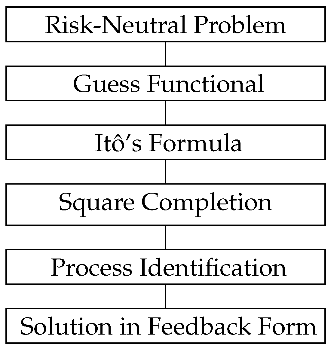(e.g., [7,8,9]) for the mean-field-free case. This approach does not use the well-known solution methods such as the stochastic maximum principle and the dynamic programming principle with Hamilton–Jacobi–Bellman–Isaacs equation and Fokker–Planck–Kolmogorov equation. It does not require extended backward–forward integro-partial differential equations (IPDEs) to solve the problem. In the risk-neutral linear–quadratic mean-field-type game, we show that there is generally a best response strategy to the mean of the state, and provide a sufficient condition of existence of mean-field Nash equilibrium. We also provide a global optimum solution to the problem in the case of full cooperation between the decision-makers. This approach gives a basic insight into the solution by providing a simple explanation for the additional term in the robust Riccati equation, compared to the risk-neutral Riccati equation. Sufficient conditions for the existence and uniqueness of mean-field equilibria are obtained when the horizon lengths are small enough and the Riccati coefficient parameters are positive. The method (see Figure 1) is then extended to the linear–quadratic robust mean-field-type games under disturbance, formulated as a minimax mean-field-type game.

Only a very limited amount of prior work seems to have been done on the MF-LQJD mean-field-type game problems. As indicated in Table 1, the jump term brings a new feature to the existing literature, and to the best of our knowledge, it is the first work that introduces and provides a bargaining solution [34] in mean-field-type games using a direct method.

The last section of this article is devoted to the validation of the novel equations derived in this article using other approaches. We confirm the validity of the optimal feedback strategies. In the Appendix we provide a basic example illustrating the sub-optimality of the mean-field game approach (which consists of freezing the mean-field term) compared with the mean-field-type game approach (in which an individual decision-maker can significantly influence the mean-field term).

1.2. Structure

A brief outline of the article follows. The next section introduces the non-cooperative mean-field-type game problem and provides its solution. Then, the fully-cooperative game and the bargaining problems and their solutions are presented. The last part of the article is devoted to adversarial problems of mean-field type.

Notation and Preliminaries

Let $T>0$ be a fixed time horizon and $(\Omega ,\mathcal{F},{\mathbb{F}}^{B,N},\mathbb{P})$ be a given filtered probability space on which a one-dimensional standard Brownian motion $B={\left\{B\left(t\right)\right\}}_{t\ge 0}$ is given, $\tilde{N}(dt,d\theta )=N(dt,d\theta )-\nu \left(d\theta \right)dt$ is a centered jump process with Lévy measure $\nu$ defined over $\Theta .$ The filtration $\mathbb{F}=\{{\mathcal{F}}_t^{B,N},0\le t\le T\}$ is the natural filtration generated by the union $\{B,N\}$ augmented by $\mathbb{P}-$null sets of $\mathcal{F}.$ The processes B and N are mutually independent. In practice, B is used to capture smaller disturbance and N is used for larger jumps of the system.

We introduce the following notation:

• Let $k\ge 1.$ $L^k(0,T;\mathbb{R})$ be the set of functions $f:[0,T]\to \mathbb{R}$ such that ${\int }_0^T{\left|f\left(t\right)\right|}^{k}dt<\infty$.
• ${\mathcal{L}}_{\mathbb{F}}^k(0,T;\mathbb{R})$ is the set of $\mathbb{F}$-adapted $\mathbb{R}$-valued processes $X(·)$ such that $E\left[{\int }_0^T{\left|X\left(t\right)\right|}^{k}dt\right]<\infty$.
• $\overline{X}\left(t\right)=E\left[X\left(t\right)\right]$ denotes the expected value of the random variable $X\left(t\right).$

An admissible control strategy $u_i$ of decision-maker i is an $\mathbb{F}$-adapted and square-integrable process with values in a non-empty subset $U_i$ of $\mathbb{R}$. We denote the set of all admissible controls by ${\mathcal{U}}_i$:

$${\mathcal{U}}_i=\{u_i(·)\in {\mathcal{L}}_{\mathbb{F}}^2(0,T;\mathbb{R});u_i(.)\in U_{i}a.e.t\in [0,T],\mathbb{P}-a.s.\}.$$

2. Non-Cooperative Problem

Consider n risk-neutral decision-makers ($n\ge 2$) and let $L_i(u_1,\dots ,u_n)$ be the objective functional of decision-maker $i,$ given by

$$\begin{array}{c}{L}_i(u_1,\dots ,u_n)=\frac{1}{2}{q}_i\left(T\right)x^2\left(T\right)+\frac{1}{2}{\overline{q}}_i\left(T\right){\left[Ex\left(T\right)\right]}^2\hfill \\ +\frac{1}{2}{\int }_0^T\left\{q_i\left(t\right)x^2\left(t\right)+{\overline{q}}_i\left(t\right){\left(E\left[x\left(t\right)\right]\right)}^2+r_i\left(t\right)u_i^2\left(t\right)+{\overline{r}}_i\left(t\right){\left[E{u}_i\left(t\right)\right]}^2\right\}dt.\hfill \end{array}$$

(1)

Then, the best-response of decision-maker i to the process $(u_{-i},E\left[x\right]):=(u_1,\dots ,u_{i-1},u_{i+1},\dots ,u_n,E\left[x\right])$ solves the following risk-neutral linear–quadratic mean-field-type control problem

$$\begin{array}{c}\hfill \left\{\begin{array}{c}\underset{u_i(·)\in {\mathcal{U}}_i}{inf}E\left[L_i(u_1,\dots ,u_n)\right],\hfill \\ {\displaystyle \mathrm{subject} \mathrm{to}}\hfill \\ dx\left(t\right)=\left\{a\left(t\right)x\left(t\right)+\overline{a}\left(t\right)E\left[x\left(t\right)\right]+\sum _{i=1}^n{b}_i\left(t\right)u_i\left(t\right)+\sum _{i=1}^n{\overline{b}}_i{\overline{u}}_i\left(t\right)\right\}dt\hfill \\ +\sigma \left(t\right)dB\left(t\right)+{\int }_{\Theta }\mu (t,\theta )\tilde{N}(dt,d\theta ),\hfill \\ x\left(0\right):=x_0,\hfill \end{array}\right.\end{array}$$

(2)

where $E{x}^2\left(0\right)<+\infty ,q_i\left(t\right)\ge 0,q_i\left(t\right)+{\overline{q}}_i\left(t\right)\ge 0,r_i\left(t\right)>0,r_i\left(t\right)+{\overline{r}}_i\left(t\right)\ge 0$, and $a\left(t\right),\overline{a}\left(t\right),b_i\left(t\right),\sigma \left(t\right)$ are real-valued functions, and where $E\left[x\right(t\left)\right]$ is the expected value of the state created by all decision-makers under the control action profile $(u_1,\dots ,u_n)\in {\prod }_{j=1}^n{\mathcal{U}}_j.$ The method below can handle time-varying coefficients. For simplicity, we impose an integrability condition on these coefficient functions over $[0,T]$:

$$\begin{array}{c}{\int }_0^T\left[\left|a\left(t\right)\right|+|\overline{a}\left(t\right)|+|b\left(t\right)|+|\overline{b}\left(t\right)|+{\sigma }^2\left(t\right)+{\int }_{\Theta }\left(\right|\mu (t,\theta )|+{\mu }^2(t,\theta ))\nu \left(d\theta \right)\right]dt<+\infty .\hfill \end{array}$$

(3)

Under condition (3), the state dynamics of (2) has a solution for each $u=(u_1,\dots ,u_n)\in {\prod }_{j=1}^n{\mathcal{U}}_j.$ Note that we do not impose boundedness or Lipschitz conditions (because quadratic functionals are not necessarily Lipschitz).

Definition 1 (BR_i: Best Response of decision-maker i).

Any strategy $u_i^{*}(·)\in {\mathcal{U}}_i$ satisfying the infimum in (2) is called a risk-neutral best-response strategy of decision-maker i to the other decision-makers strategy $u_{-i}\in {\prod }_{j\ne i}{\mathcal{U}}_j.$ The set of best-response strategies of i is denoted by $B{R}_i:{\prod }_{j\ne i}{\mathcal{U}}_j\to 2^{{\mathcal{U}}_i},$ where $2^{{\mathcal{U}}_i}$ denotes the set of subsets of ${\mathcal{U}}_i.$

Note that if $b_i=0=r_i$, there are multiple optimizers of the best-response problem.

Definition 2 (Mean-Field Nash Equilibrium).

Any strategy profile $(u_i^{*},\dots ,u_n^{*})\in {\prod }_i{\mathcal{U}}_i$ such that $u_i^{*}\in B{R}_i\left(u_{-i}^{*}\right)$ for every i and ${\overline{x}}^{*}=E\left[x^{*}\right]$ is called a Nash equilibrium of the LQ-MFJD game above.

The risk-neutral mean-field-type Nash equilibrium problem we are concerned with is to find and characterize the processes $(x^{*},u^{*},E\left[x^{*}\right],E\left[u^{*}\right])$ such that for every decision-maker $i,$ $u_i^{*}$ is an optimizer of the best response problem (2) and the expected value of the resulting common state $E\left[x^{*}\right]$ created by all the decision-makers coincides with $\overline{x}.$ This means that an equilibrium is a fixed-point of the best response correspondence $BR=(B{R}_1,\dots ,B{R}_n)$, where $B{R}_i:{\prod }_{j\ne i}{\mathcal{U}}_j\to 2^{{\mathcal{U}}_i}$ is the best-response correspondence of decision-maker $i.$

We rewrite the expected objective functional and the state coefficients in terms of $x-\overline{x}$ and $\overline{x}:$

$$\begin{array}{c}E{L}_i=\frac{1}{2}[q_i\left(T\right)E{(x\left(T\right)-\overline{x}\left(T\right))}^2+[q_i\left(T\right)+{\overline{q}}_i\left(T\right)]{\overline{x}}^2\left(T\right)\hfill \\ +E{\int }_0^T{q}_i{(x-\overline{x})}^2+[q_i+{\overline{q}}_i]{\overline{x}}^2+r_i{(u_i-{\overline{u}}_i)}^2+(r_i+{\overline{r}}_i){\left[{\overline{u}}_i\right]}^{2}dt],\hfill \\ dx=\left\{a(x-\overline{x})+(a+\overline{a})\overline{x}+\sum _{i=1}^n{b}_i(u_i-{\overline{u}}_i)+\sum _{i=1}^n(b_i+{\overline{b}}_i){\overline{u}}_i\right\}dt\hfill \\ +\sigma dB\left(t\right)+{\int }_{\Theta }\mu (t,\theta )\tilde{N}(dt,d\theta ).\hfill \end{array}$$

(4)

Note that the expected value of the first term in the integral in $L_i$ can be seen as a weighted variance $var$ of the state, since ${\overline{q}}_i\left(t\right)E\left[{(x\left(t\right)-E\left[x\left(t\right)\right])}^2\right]={\overline{q}}_i\left(t\right)var\left(x\left(t\right)\right).$ Taking the expectation of the state dynamics, one arrives at the deterministic linear dynamics

$$\begin{array}{c}\frac{d}{dt}Ex=\dot{\overline{x}}=(a+\overline{a})\overline{x}+\sum _{i=1}^n(b_i+{\overline{b}}_i){\overline{u}}_i,\hfill \\ \overline{x}\left(0\right)=Ex\left(0\right).\hfill \end{array}$$

(5)

The direct method consists of writing a generic structure of the cost functional, with unknown deterministic functions to be identified. Inspired from the structure of the terminal cost function, we try a generic solution in a quadratic form. Let $f_i(t,x)=\frac{1}{2}{\alpha }_i\left(t\right){(x-\overline{x})}^2+\frac{1}{2}{\beta }_i\left(t\right){\overline{x}}^2+{\gamma }_i\left(t\right)\overline{x}+{\delta }_i\left(t\right),$ where $\alpha ,$ $\beta ,\gamma ,\delta$ are deterministic functions of time, such that

$$f_i(T,x\left(T\right))=\frac{1}{2}\{q_i\left(T\right)E{(x\left(T\right)-\overline{x}\left(T\right))}^2+[q_i\left(T\right)+{\overline{q}}_i\left(T\right)]{\overline{x}}^2\left(T\right)\}.$$

At the final time $T,$ one can identify ${\alpha }_i\left(T\right)=q_i\left(T\right),{\beta }_i\left(T\right)=q_i\left(T\right)+{\overline{q}}_i\left(T\right),{\gamma }_i\left(T\right)={\delta }_i\left(T\right)=0.$

Recall that Itô’s formula for the jump-diffusion process is

$$\begin{array}{c}{f}_i(T,x\left(T\right))=f_i(0,x\left(0\right))\hfill \\ +{\int }_0^T[f_{i,t}+f_{i,x}D+f_{i,xx}\frac{{\sigma }^2}{2}]dt\hfill \\ +{\int }_0^T\sigma f_{i,x}dB\hfill \\ +{\int }_0^T{\int }_{\Theta }[f_i(t,x+\mu (t,\theta ))-f_i(t,x)-f_{i,x}\mu (t,\theta )]\nu \left(d\theta \right)dt\hfill \\ +{\int }_0^T{\int }_{\Theta }[f_i(t_{-},x+\mu (t_{-},\theta ))-f_i(t_{-},x)]\tilde{N}(dt,d\theta ),\hfill \end{array}$$

(6)

where D is the drift term $D:=a(x-\overline{x})+(a+\overline{a})\overline{x}+{\sum }_{i=1}^n{b}_i(u_i-{\overline{u}}_i)+{\sum }_{i=1}^n(b_i+{\overline{b}}_i){\overline{u}}_i$. We compute the derivative terms:

$$\left\{\begin{array}{c}\dot{\overline{x}}=(a+\overline{a})\overline{x}+\sum _{i=1}^n(b_i+{\overline{b}}_i){\overline{u}}_i,\hfill \\ f_{i,t}=\frac{1}{2}{\dot{\alpha }}_i{(x-\overline{x})}^2+\frac{1}{2}{\dot{\beta }}_i{\overline{x}}^2+{\dot{\gamma }}_i\overline{x}+{\dot{\delta }}_i-{\alpha }_i(x-\overline{x})\dot{\overline{x}}+{\beta }_i\overline{x}\dot{\overline{x}}+{\gamma }_i\dot{\overline{x}},\hfill \\ f_{i,x}={\dot{\alpha }}_i(x-\overline{x}),\hfill \\ f_{i,xx}={\alpha }_i,\hfill \\ f_i(t,x+\mu )-f_i(t,x)-f_{i,x}\mu \hfill \\ =\frac{1}{2}{\alpha }_i{(x+\mu -\overline{x})}^2-\frac{1}{2}{\alpha }_i{(x-\overline{x})}^2-{\alpha }_i(x-\overline{x})\mu =\frac{1}{2}{\alpha }_i{\mu }^2.\hfill \end{array}\right.$$

(7)

Using (7) in (6) and taking the expectation yields

$$\begin{array}{c}E[f_i(T,x\left(T\right))-f_i(0,x\left(0\right))]\hfill \\ =\frac{1}{2}E{\int }_0^T{\dot{\alpha }}_i{(x-\overline{x})}^2+{\dot{\beta }}_i{\overline{x}}^{2}dt\hfill \\ +\frac{1}{2}E{\int }_0^{T}2{\beta }_i[(a+\overline{a}){\overline{x}}^2+\sum _{j=1}^n(b_j+{\overline{b}}_j){\overline{u}}_j\overline{x}]dt\hfill \\ +\frac{1}{2}E{\int }_0^T\left\{2a{\alpha }_i{(x-\overline{x})}^2+2{\alpha }_i\sum _{j=1}^n{b}_j(u_j-{\overline{u}}_j)(x-\overline{x})\right\}dt\hfill \\ +\frac{1}{2}{\int }_0^T\left[{\sigma }^2+{\int }_{\Theta }{\mu }^2(t,\theta )\nu \left(d\theta \right)\right]{\alpha }_{i}dt\hfill \\ +E{\int }_0^T{\dot{\gamma }}_i\overline{x}+{\gamma }_i[(a+\overline{a})\overline{x}+\sum _{j=1}^n(b_j+{\overline{b}}_j){\overline{u}}_j]dt+{\int }_0^T{\dot{\delta }}_{i}dt,\hfill \end{array}$$

(8)

where we have used the following equalities:

$$\left\{\begin{array}{c}E\left[{\alpha }_i(x-\overline{x})\dot{\overline{x}}\right]=0,\hfill \\ E{\int }_0^T\sigma f_{i,x}dB=0,\hfill \\ E{\int }_0^T{\int }_{\Theta }[f_i(t,x+\mu (t,\theta ))-f_i(t,x)]\tilde{N}(dt,d\theta )=0.\hfill \end{array}\right.$$

(9)

We compute the gap between $E\left[L_i\right]$ and $E\left[f_i(0,x\left(0\right))\right]$ as

$$\begin{array}{c}E[L_i-f_i(0,x\left(0\right))]\hfill \\ =\frac{1}{2}(q_i\left(T\right)-{\alpha }_i\left(T\right))E{(x\left(T\right)-\overline{x}\left(T\right))}^2\hfill \\ +\frac{1}{2}[q_i\left(T\right)+{\overline{q}}_i\left(T\right)-{\beta }_i\left(T\right)]{\overline{x}}^2\left(T\right)\hfill \\ +\frac{1}{2}E{\int }_0^T{q}_i{(x-\overline{x})}^2+[q_i+{\overline{q}}_i]{\overline{x}}^2\left(t\right)dt\hfill \\ +\frac{1}{2}E{\int }_0^T{r}_i{(u_i-{\overline{u}}_i\left(t\right))}^2+(r_i+{\overline{r}}_i){\left[{\overline{u}}_i\right]}^{2}dt]\hfill \\ +\frac{1}{2}E{\int }_0^T{\dot{\alpha }}_i{(x-\overline{x})}^2+{\dot{\beta }}_i{\overline{x}}^2+2{\beta }_i(a+\overline{a}){\overline{x}}^{2}dt\hfill \\ +\frac{1}{2}E{\int }_0^{T}2{\beta }_i(b_i+{\overline{b}}_i){\overline{u}}_i\overline{x}dt\hfill \\ +\frac{1}{2}E{\int }_0^{T}2{\beta }_i\sum _{j\ne i}^n(b_j+{\overline{b}}_j){\overline{u}}_j\overline{x}dt\hfill \\ +\frac{1}{2}E{\int }_0^T\left\{2a{\alpha }_i{(x-\overline{x})}^2+2{\alpha }_i{b}_i(u_i-{\overline{u}}_i)(x-\overline{x})+2{\alpha }_i\sum _{j\ne i}{b}_j(u_j-{\overline{u}}_j)(x-\overline{x})\right\}dt\hfill \\ +\frac{1}{2}{\int }_0^T\left[{\sigma }^2+{\int }_{\Theta }{\mu }^2(t,\theta )\nu \left(d\theta \right)\right]{\alpha }_{i}dt\hfill \\ +\frac{1}{2}E{\int }_0^{T}2{\dot{\gamma }}_i\overline{x}+2{\gamma }_i[(a+\overline{a})\overline{x}+\sum _{j=1}^n(b_j+{\overline{b}}_j){\overline{u}}_j]dt\hfill \\ +\frac{1}{2}{\int }_0^{T}2{\dot{\delta }}_{i}dt.\hfill \end{array}$$

(10)

2.1. Best Response to Open-Loop Strategies

In this subsection, we compute the best-response of decision-maker i to open-loop strategies ${\left(u_j\right)}_{j\ne i}.$ The information structure for the others players is limited to time and initial point; i.e., the mappings ${\left(u_j\right)}_{j\ne i}$ are measurable functions of time (and do not depend on x) and initial point $x_0.$

$$\begin{array}{c}E[L_i-f_i(0,x\left(0\right))]\hfill \\ =\frac{1}{2}[(q_i\left(T\right)-{\alpha }_i\left(T\right))E{(x\left(T\right)-\overline{x}\left(T\right))}^2\hfill \\ +\frac{1}{2}[q_i\left(T\right)+{\overline{q}}_i\left(T\right)-{\beta }_i\left(T\right)]{\overline{x}}^2\left(T\right)\hfill \\ +\frac{1}{2}E{\int }_0^T\{{\dot{\alpha }}_i+2a{\alpha }_i-\frac{b_i^2}{r_i}{\alpha }_i^2+q_i\}{(x\left(t\right)-\overline{x}\left(t\right))}^2\hfill \\ +\frac{1}{2}E{\int }_0^T[{\dot{\beta }}_i+2{\beta }_i(a+\overline{a})-\frac{{(b_i+{\overline{b}}_i)}^2}{r_i+{\overline{r}}_i}{\beta }_i^2+q_i+{\overline{q}}_i]{\overline{x}}^{2}dt\hfill \\ +\frac{1}{2}E{\int }_0^T{r}_i{[u_i-{\overline{u}}_i+\frac{b_i}{r_i}{\alpha }_i(x-\overline{x})]}^{2}dt\hfill \\ +\frac{1}{2}E{\int }_0^T(r_i+{\overline{r}}_i){[{\overline{u}}_i+\frac{(b_i+{\overline{b}}_i)}{r_i+{\overline{r}}_i}({\beta }_i\overline{x}+{\gamma }_i)]}^{2}dt\hfill \\ +\frac{1}{2}E{\int }_0^T\left\{2{\dot{\gamma }}_i+2{\gamma }_i(a+\overline{a})-\frac{{(b_i+{\overline{b}}_i)}^2}{r_i+{\overline{r}}_i}2{\beta }_i{\gamma }_i+2{\beta }_i\sum _{j\ne i}(b_j+{\overline{b}}_j){\overline{u}}_j\right\}\overline{x}dt\hfill \\ +\frac{1}{2}E{\int }_0^T-\frac{{(b_i+{\overline{b}}_i)}^2}{r_i+{\overline{r}}_i}{\gamma }_i^2+2{\gamma }_i\sum _{j\ne i}(b_j+{\overline{b}}_j){\overline{u}}_{j}dt\hfill \\ +\frac{1}{2}{\int }_0^T\left[{\sigma }^2+{\int }_{\Theta }{\mu }^2(t,\theta )\nu \left(d\theta \right)\right]{\alpha }_{i}dt\hfill \\ +\frac{1}{2}{\int }_0^{T}2{\dot{\delta }}_{i}dt,\hfill \end{array}$$

(11)

where

$$\begin{array}{c}(r_i+{\overline{r}}_i){\left[{\overline{u}}_i\right]}^2+2{\beta }_i\sum _{j=1}^n(b_j+{\overline{b}}_j){\overline{u}}_j\overline{x}+2{\gamma }_i\sum _{j=1}^n(b_j+{\overline{b}}_j){\overline{u}}_j\hfill \\ =(r_i+{\overline{r}}_i){\left[{\overline{u}}_i\right]}^2+2{\overline{u}}_i(b_i+{\overline{b}}_i)({\beta }_{i}x+{\overline{\gamma }}_i)+2{\beta }_i\sum _{j\ne i}(b_j+{\overline{b}}_j){\overline{u}}_j\overline{x}+2{\gamma }_i\sum _{j\ne i}(b_j+{\overline{b}}_j){\overline{u}}_j\hfill \\ =(r_i+{\overline{r}}_i){[{\overline{u}}_i+\frac{(b_i+{\overline{b}}_i)}{r_i+{\overline{r}}_i}({\beta }_i\overline{x}+{\gamma }_i)]}^2-\frac{{(b_i+{\overline{b}}_i)}^2}{r_i+{\overline{r}}_i}\{{\beta }_i^2{\overline{x}}^2+2{\beta }_i{\gamma }_i\overline{x}+{\overline{\gamma }}_i^2\}\hfill \\ +2{\beta }_i\sum _{j\ne i}(b_j+{\overline{b}}_j){\overline{u}}_j\overline{x}+2{\gamma }_i\sum _{j\ne i}(b_j+{\overline{b}}_j){\overline{u}}_j.\hfill \end{array}$$

(12)

The best response of decision-maker i to the open-loop strategies ${\left(u_j\right)}_{j\ne i}$ is $u_i={\overline{u}}_i-\frac{b_i}{r_i}{\alpha }_i(x-\overline{x})$, and its expected value is ${\overline{u}}_i=-\frac{(b_i+{\overline{b}}_i)}{r_i+{\overline{r}}_i}({\beta }_i\overline{x}+{\gamma }_i)$, where ${\alpha }_i,{\beta }_i,{\gamma }_i$ are deterministic functions of time $t.$ Clearly, the best response to open-loop strategies is in state-and-mean-field feedback form. Here the mean-field feedback terms are the expected value of the state $E\left[x\right(t\left)\right]$ and the expected value of the control action $E\left[u_i\left(t\right)\right].$

Therefore, we examine optimal strategies in state-and-mean-field feedback form in the next section.

2.2. Feedback Strategies

The information structure for feedback solution is as follows. The model and the objective functions are assumed to be common knowledge. We assume that the state is of perfect observation. We will show below that the mean-field term is computable (via the initial mean state and the model). If the other decision-makers play their optimal state-and-mean-field feedback strategies, then the functions ${\gamma }_1,\dots ,{\gamma }_n$ are identically zero at any given time. We compute again $E[L_i-f_i(0,x\left(0\right))]$ and complete the squares using the elements of $\{x-\overline{x},\overline{x}\}.$

$$\begin{array}{c}E[L_i-f_i(0,x\left(0\right))]\hfill \\ =\frac{1}{2}(q_i\left(T\right)-{\alpha }_i\left(T\right))E{(x\left(T\right)-\overline{x}\left(T\right))}^2\hfill \\ +\frac{1}{2}[q_i\left(T\right)+{\overline{q}}_i\left(T\right)-{\beta }_i\left(T\right)]{\overline{x}}^2\left(T\right)\hfill \\ +\frac{1}{2}E{\int }_0^T[{\dot{\alpha }}_i+2a{\alpha }_i-\frac{b_i^2}{r_i}{\alpha }_i^2-2{\alpha }_i\sum _{j\ne i}^n\frac{b_j^2}{r_j}{\alpha }_j+q_i]{(x-\overline{x})}^2\hfill \\ +\frac{1}{2}E{\int }_0^T\left\{{\dot{\beta }}_i+2{\beta }_i(a+\overline{a})-{\beta }_i^2\frac{{(b_i+{\overline{b}}_i)}^2}{r_i+{\overline{r}}_i}-2{\beta }_i\sum _{j\ne i}^n\frac{{(b_j+{\overline{b}}_j)}^2}{r_j+{\overline{r}}_j}{\beta }_j+q_i+{\overline{q}}_i\right\}{\overline{x}}^{2}dt\hfill \\ +\frac{1}{2}E{\int }_0^T{r}_i{[u_i-{\overline{u}}_i+\frac{b_i}{r_i}{\alpha }_i(x-\overline{x})]}^{2}dt\hfill \\ +\frac{1}{2}E{\int }_0^T(r_i+{\overline{r}}_i){[{\overline{u}}_i+{\beta }_i\frac{(b_i+{\overline{b}}_i)}{r_i+{\overline{r}}_i}\overline{x}]}^{2}dt\hfill \\ +\frac{1}{2}E{\int }_0^T\left[{\sigma }^2+{\int }_{\Theta }{\mu }^2(t,\theta )\nu \left(d\theta \right)\right]{\alpha }_{i}dt,\hfill \end{array}$$

(13)

where we have used the following square completions:

$$\begin{array}{c}{r}_i{(u_i-{\overline{u}}_i)}^2+2{\alpha }_i\sum _{j=1}^n{b}_j(u_j-{\overline{u}}_j)(x-\overline{x})\hfill \\ =r_i{[u_i-{\overline{u}}_i+\frac{b_i}{r_i}{\alpha }_i(x-\overline{x})]}^2-\frac{b_i^2}{r_i}{\alpha }_i^2{(x-\overline{x})}^2+2{\alpha }_i\sum _{j\ne i}{b}_j(u_j-{\overline{u}}_j)(x-\overline{x}),\mathrm{and}\hfill \\ (r_i+{\overline{r}}_i){\left[{\overline{u}}_i\right]}^2+2{\beta }_i\sum _{j=1}^n(b_j+{\overline{b}}_j){\overline{u}}_j\overline{x}\hfill \\ =(r_i+{\overline{r}}_i){[{\overline{u}}_i+{\beta }_i\frac{(b_i+{\overline{b}}_i)}{r_i+{\overline{r}}_i}\overline{x}]}^2-{\beta }_i^2\frac{{(b_i+{\overline{b}}_i)}^2}{r_i+{\overline{r}}_i}{\overline{x}}^2+2{\beta }_i\sum _{j\ne i}(b_j+{\overline{b}}_j){\overline{u}}_j\overline{x}.\hfill \end{array}$$

(14)

It follows that

$$\begin{array}{c}\underset{u_i\in {\mathcal{U}}_i}{inf}E\left[L_i\right]=\frac{1}{2}{\alpha }_i\left(0\right)var\left(x\left(0\right)\right)+\frac{1}{2}{\beta }_i\left(0\right){\left[Ex\left(0\right)\right]}^2+\frac{1}{2}{\int }_0^T\left[{\sigma }^2+{\int }_{\Theta }{\mu }^2(t,\theta )\nu \left(d\theta \right)\right]{\alpha }_{i}dt,\hfill \\ u_i^{*}=-\frac{b_i}{r_i}{\alpha }_i(x-\overline{x})-{\beta }_i\frac{(b_i+{\overline{b}}_i)}{r_i+{\overline{r}}_i}\overline{x},\hfill \\ {\dot{\alpha }}_i+2a{\alpha }_i-\frac{b_i^2}{r_i}{\alpha }_i^2-2{\alpha }_i\sum _{j\ne i}\frac{b_j^2}{r_j}{\alpha }_j+q_i=0,\hfill \\ {\alpha }_i\left(T\right)=q_i\left(T\right),\hfill \\ {\dot{\beta }}_i+2{\beta }_i(a+\overline{a})-{\beta }_i^2\frac{{(b_i+{\overline{b}}_i)}^2}{r_i+{\overline{r}}_i}-2{\beta }_i\sum _{j\ne i}\frac{{(b_j+{\overline{b}}_j)}^2}{r_j+{\overline{r}}_j}{\beta }_j+q_i+{\overline{q}}_i=0,\hfill \\ {\beta }_i\left(T\right)=q_i\left(T\right)+{\overline{q}}_i\left(T\right).\hfill \\ \overline{x}\left(t\right)=\overline{x}\left(0\right)e^{{\int }_0^t\{(a+\overline{a})-{\sum }_{i=1}^n{\beta }_i\frac{{(b_i+{\overline{b}}_i)}^2}{r_i+{\overline{r}}_i}\}d{t}^{\prime }}\hfill \end{array}$$

(15)

provides a mean-field Nash equilibrium in feedback strategies.

These Riccati equations are different from those of open-loop control strategies. The coefficient of the coupling terms ${\beta }_i{\beta }_j,{\alpha }_i{\alpha }_j$ are different, reflecting the coupling through the state and the mean state. Notice that the optimal strategy is in state-and-mean-field feedback form, which is different from the standard LQG game solution. As $\overline{a},\overline{b},\overline{r},\overline{q}$ vanish in (15), one gets the Nash equilibrium of the corresponding stochastic differential game in closed-loop strategies with ${\alpha }_i={\beta }_i,$ and $u_i$ becomes mean-field-free. When the diffusion coefficient $\sigma$ and the jump rate $\mu$ vanish, one obtains the noiseless deterministic game problem, and the optimal strategy solution will be given by the equation in ${\beta }_i$ because $x-\overline{x}=0$ in the deterministic case.

How to feedback the mean-field term $E\left[x\right(t\left)\right]$? Here the mean-field term can be explicitly computed if the initial mean state $\overline{x}\left(0\right)$ is given and the model known:

$$E\left[x\left(t\right)\right]=\overline{x}\left(t\right)=\overline{x}\left(0\right)e^{{\int }_0^t\{(a+\overline{a})-{\sum }_{i=1}^n{\beta }_i\frac{{(b_i+{\overline{b}}_i)}^2}{r_i+{\overline{r}}_i}\}d{t}^{\prime }}.$$

3. Fully-Cooperative Solutions

In this section, we examine the global optimum and Nash bargaining solution [34] of the game.

3.1. Global Optimum

We now consider the fully cooperative scenario where all the decision-makers decide jointly to optimize a single global objective $L_0:={\sum }_i{L}_i$ given by

$$\begin{array}{c}\underset{(u_1,\dots ,u_n)}{inf}E\sum _i{L}_i,\hfill \\ dx=\left\{a(x-\overline{x})+(a+\overline{a})\overline{x}+\sum _{i=1}^n{b}_i(u_i-{\overline{u}}_i)+\sum _{i=1}^n(b_i+{\overline{b}}_i){\overline{u}}_i\right\}dt\hfill \\ +\sigma dB\left(t\right)+{\int }_{\Theta }\mu (t,\theta )\tilde{N}(dt,d\theta ),\hfill \\ x\left(0\right)=x_0.\hfill \end{array}$$

(16)

Following the same methodology as above with $q_0={\sum }_i{q}_i,{\overline{q}}_0={\sum }_i{\overline{q}}_i$ and $f_0(t,x)=\frac{1}{2}{\alpha }_0\left(t\right){(x-\overline{x})}^2+\frac{1}{2}{\beta }_0\left(t\right){\overline{x}}^2,$ we obtain:

$$\begin{array}{c}\underset{(u_1,\dots ,u_n)}{inf}E\sum _i\left[L_i\right]\hfill \\ =\frac{1}{2}{\alpha }_0\left(0\right)var\left(x\left(0\right)\right)+\frac{1}{2}{\beta }_0\left(0\right){\left[Ex\left(0\right)\right]}^2+\frac{1}{2}{\int }_0^T\left[{\sigma }^2\left(t\right)+{\int }_{\Theta }{\mu }^2(t,\theta )\nu \left(d\theta \right)\right]{\alpha }_0\left(t\right)dt,\hfill \\ u_i^{*}=-\frac{b_i}{r_i}{\alpha }_0(x-\overline{x})-{\beta }_0\frac{(b_i+{\overline{b}}_i)}{r_i+{\overline{r}}_i}\overline{x},\hfill \\ {\dot{\alpha }}_0+2a{\alpha }_0-{\alpha }_0^2\sum _i\frac{b_i^2}{r_i}+q_0=0,\hfill \\ {\alpha }_0\left(T\right)=q_0\left(T\right)=\sum _{i=1}^n{q}_i\left(T\right),\hfill \\ {\dot{\beta }}_0+2{\beta }_0(a+\overline{a})-{\beta }_0^2\sum _{i=1}^n\frac{{(b_i+{\overline{b}}_i)}^2}{r_i+{\overline{r}}_i}+q_0+{\overline{q}}_0=0,\hfill \\ {\beta }_0\left(T\right)=\sum _{i=1}^n{q}_i\left(T\right)+{\overline{q}}_i\left(T\right).\hfill \\ \overline{x}\left(t\right)=\overline{x}\left(0\right)e^{{\int }_0^t\{(a+\overline{a})-{\beta }_0{\sum }_{i=1}^n\frac{{(b_i+{\overline{b}}_i)}^2}{r_i+{\overline{r}}_i}\}d{t}^{\prime }}.\hfill \end{array}$$

(17)

When the coefficients are constant (in time), ${\alpha }_0,{\beta }_0$ are explicitly given by

$$\begin{array}{c}S:=\sum _i\frac{b_i^2}{r_i},\hfill \\ {\alpha }_0\left(t\right)=\frac{a}{S}+\sqrt{\frac{q_0}{S}+\frac{a^2}{S^2}}\left(-1+\frac{q_0\left(T\right)-\frac{a}{S}+\sqrt{\frac{q_0}{S}+\frac{a^2}{S^2}}}{\Gamma }\right),\hfill \\ \Gamma :=\frac{1}{2}(q_0\left(T\right)-\frac{a}{S}+\sqrt{\frac{q_0}{S}+\frac{a^2}{S^2}})-\frac{1}{2}(q_0\left(T\right)-\frac{a}{S}-\sqrt{\frac{q_0}{S}+\frac{a^2}{S^2}})e^{-2(T-t)\sqrt{\frac{q_0}{S}+\frac{a^2}{S^2}}},\hfill \\ \tilde{S}:=\sum _{i=1}^n\frac{{(b_i+{\overline{b}}_i)}^2}{r_i+{\overline{r}}_i},\hfill \\ {\beta }_0\left(t\right)=\frac{a+\overline{a}}{\tilde{S}}+\sqrt{\frac{q_0+{\overline{q}}_0}{\tilde{S}}+\frac{a^2}{{\tilde{S}}^2}}\left(-1+\frac{q_0\left(T\right)+{\overline{q}}_0\left(T\right)-\frac{a+\overline{a}}{\tilde{S}}+\sqrt{\frac{q_0+{\overline{q}}_0}{\tilde{S}}+\frac{{(a+\overline{a})}^2}{{\tilde{S}}^2}}}{\tilde{\Gamma }}\right),\hfill \\ \tilde{\Gamma }:=\frac{1}{2}(q_0\left(T\right)+{\overline{q}}_0\left(T\right)-\frac{a+\overline{a}}{\tilde{S}}+\sqrt{\frac{q_0+{\overline{q}}_0}{\tilde{S}}+\frac{{(a+\overline{a})}^2}{{\tilde{S}}^2}})\hfill \\ -\frac{1}{2}(q_0\left(T\right)+{\overline{q}}_0\left(T\right)-\frac{a+\overline{a}}{\tilde{S}}-\sqrt{\frac{q_0+{\overline{q}}_0}{\tilde{S}}+\frac{{(a+\overline{a})}^2}{{\tilde{S}}^2}})\times e^{-2(T-t)\sqrt{\frac{q_0+{\overline{q}}_0}{\tilde{S}}+\frac{{(a+\overline{a})}^2}{{\tilde{S}}^2}}}.\hfill \end{array}$$

(18)

The global optimum cost in the fully-cooperative case is

$$\begin{array}{c}{L}_0=\frac{1}{2}{\alpha }_0\left(0\right)var\left(x\left(0\right)\right)+\frac{1}{2}{\beta }_0\left(0\right){\left[Ex\left(0\right)\right]}^2+\frac{1}{2}{\int }_0^T\left[{\sigma }^2\left(t\right)+{\int }_{\Theta }{\mu }^2(t,\theta )\nu \left(d\theta \right)\right]{\alpha }_0\left(t\right)dt,\hfill \end{array}$$

(19)

and is less than the total cost at the Nash equilibrium, which is

$$\begin{array}{c}\frac{1}{2}\left(\sum _{i=1}^n{\alpha }_i\left(0\right)\right)var\left(x\left(0\right)\right)+\frac{1}{2}\left(\sum _{i=1}^n{\beta }_i\left(0\right)\right){\left(\overline{x}\left(0\right)\right)}^2+\frac{1}{2}{\int }_0^T\left[{\sigma }^2\left(t\right)+{\int }_{\Theta }{\mu }^2(t,\theta )\nu \left(d\theta \right)\right]\sum _{i=1}^n{\alpha }_i\left(t\right)dt.\hfill \end{array}$$

(20)

This loss of efficiency of Nash equilibria was analyzed in [35], and is often termed as the price of anarchy [36,37].

3.2. Nash Bargaining Solution

Mean-field-type bargaining theory deals with the situation in which decision-makers can realize—through cooperation—other better outcomes than the one which becomes effective when they do not cooperate. This non-cooperative outcome is called the threatpoint $L^{NE}=(L_1^{NE},\dots ,L_n^{NE})$. The question is which outcome might the decision-makers possibly agree to. Let $\mathcal{V}$ be the set of feasible outcomes of the benefit of bargaining [34]. We assume that if the agents unanimously agree on a point $v=(v_1,\dots ,v_n)\in \mathcal{V},$ they obtain $v.$ Otherwise, they obtain $L^{NE}=(L_1^{NE},\dots ,L_n^{NE}).$ This presupposes that each decision-maker can enforce the threatpoint when he does not agree with a proposal. Generically, what decision-maker i can guarantee is ${inf}_{u_i}{sup}_{u_{-i}}{L}_i$, which is non-admissible in the quadratic setting. The outcome v the decision-makers will finally agree on is called the solution of the bargaining problem. Therefore, we have chosen the non-cooperation solution when there is a disagreement.

The Nash bargaining solution selects for a given set $\mathcal{V}$ the point at which the product of gains from $L^{NE}$ is maximal.

$$NBS(\mathcal{V},L^{NE})=arg\underset{v\in \mathcal{V}}{max}\left\{\prod _{i\in \mathcal{N}}[L_i^{NE}-v_i]\right\}$$

(21)

Since the function $v\mapsto {\prod }_{k\in \mathcal{N}}{v}_k$ is non-convex, Problem (21) is non-convex. Here we exploit the convexity of the functional $u\mapsto \langle w,L\left(u\right)\rangle$ for any given $w=(w_1,\dots ,w_n)\in {\mathbb{R}}_{++}^n$ such that ${\sum }_{i=1}^n{w}_i=1$ to reach any point in the Pareto frontier of the game. The maximization (in w) of the product $P:={\prod }_{i=1}^n[L_i^{NE}-L_i\left(\widehat{u}\left(w\right)\right)]$ yields

$$\sum _{i=1}^n\frac{\partial }{\partial w_j}{L}_i\left(\widehat{u}\left(w\right)\right).\left\{\prod _{j\ne i}[L_j^{NE}-L_j\left(\widehat{u}\left(w\right)\right)]\right\}=c.$$

This is equivalent to

$$\sum _{i=1}^n\frac{P}{L_i^{NE}-L_i\left(\widehat{u}\left(w\right)\right)}\frac{\partial }{\partial w_j}{L}_i\left(\widehat{u}\left(w\right)\right)=c.$$

We set $y_i:=\frac{\frac{P}{L_i^{NE}-L_i\left(\widehat{u}\left(w\right)\right)}}{{\sum }_{k=1}^n\left(\frac{P}{L_k^{NE}-L_k\left(\widehat{u}\left(w\right)\right)}\right)}.$ Then, it follows that

$$\sum _{i=1}^n{y}_i\frac{\partial }{\partial w_j}{L}_i\left(\widehat{u}\left(w\right)\right)=\frac{c}{{\sum }_{i=1}^n\left(\frac{P}{L_i^{NE}-L_i\left(\widehat{u}\left(w\right)\right)}\right)}.$$

Moreover, $y_i\ge 0,{\sum }_{i=1}^n{y}_i=1.$

Assume the matrix ${\left(\frac{\partial }{\partial w_j}{L}_i\left(\widehat{u}\left(w\right)\right)\right)}_{(i,j)\in {\mathcal{N}}^2}$ has at least rank $n-1.$ Then, the Nash bargaining solution is explicitly given by $v=(L_1\left(\widehat{u}\left(w^{*}\right)\right),\dots ,L_n\left(\widehat{u}\left(w^{*}\right)\right))$, with the weight

$$w_i^{*}=\frac{{\prod }_{j\ne i}[L_j^{NE}-L_j\left(\widehat{u}\left(w^{*}\right)\right)]}{{\sum }_{k=1}^n{\prod }_{j\ne k}[L_j^{NE}-L_j\left(\widehat{u}\left(w^{*}\right)\right)]}=y_i\left(w^{*}\right),$$

where the optimal bargaining strategy profile is $\widehat{u}\left(w\right)\in arg{min}_u\left\{\langle w,L\left(u\right)\rangle \right\}.$ It remains to compute the functional $\widehat{u}\left(w\right)=({\widehat{u}}_1\left(w\right),\dots ,{\widehat{u}}_n\left(w\right)).$

$$\begin{array}{c}\underset{(u_1,\dots ,u_n)}{inf}E\sum _i{w}_i{L}_i,\hfill \\ dx=\left\{a(x-\overline{x})+(a+\overline{a})\overline{x}+\sum _{i=1}^n{b}_i(u_i-{\overline{u}}_i)+\sum _{i=1}^n(b_i+{\overline{b}}_i){\overline{u}}_i\right\}dt\hfill \\ +\sigma dB+{\int }_{\Theta }\mu (t,\theta )\tilde{N}(dt,d\theta ).\hfill \\ x\left(0\right)=x_0,\hfill \end{array}$$

(22)

Following the same methodology as above, we obtain:

$$\begin{array}{c}\underset{(u_1,\dots ,u_n)}{inf}E\sum _i{w}_i{L}_i=\frac{1}{2}{\alpha }_0\left(0\right)var\left(x\left(0\right)\right)+\frac{1}{2}{\beta }_0\left(0\right){\left[\overline{x}\left(0\right)\right]}^2+{\int }_0^T\left[{\sigma }^2+{\int }_{\Theta }{\mu }^2(t,\theta )\nu \left(d\theta \right)\right]\frac{{\alpha }_0}{2}dt,\hfill \\ {\widehat{u}}_i\left(w\right)=-\frac{b_i}{w_i{r}_i}{\alpha }_0(x-\overline{x})-\frac{(b_i+{\overline{b}}_i)}{w_i(r_i+{\overline{r}}_i)}\left({\beta }_0\overline{x}\right),\hfill \\ {\dot{\alpha }}_0+2a{\alpha }_0-{\alpha }_0^2\sum _i\frac{b_i^2}{w_i{r}_i}+\sum _i{w}_i{q}_i=0,\hfill \\ {\alpha }_0\left(T\right)=\sum _i{w}_i{q}_i\left(T\right),\hfill \\ {\dot{\beta }}_0+2{\beta }_0(a+\overline{a})-{\beta }_0^2\sum _i\frac{{(b_i+{\overline{b}}_i)}^2}{w_i(r_i+{\overline{r}}_i)}+\sum _i{w}_i(q_i+{\overline{q}}_i)=0,\hfill \\ {\beta }_0\left(T\right)=\sum _i{w}_i(q_i+{\overline{q}}_i\left(T\right)),\hfill \\ \overline{x}\left(t\right)=\overline{x}\left(0\right)e^{{\int }_0^t[a+\overline{a}-{\beta }_0{\sum }_{i=1}^n\frac{{(b_i+{\overline{b}}_i)}^2}{w_i(r_i+{\overline{r}}_i)}]d{t}^{\prime }},\hfill \\ \overline{x}\left(0\right)\in \mathbb{R}.\hfill \end{array}$$

(23)

4. LQ Robust Mean-Field-Type Games

We now consider a robust mean-field-type game with two decision-makers. Decision-maker 1 minimizes with respect to $u_1$ and Decision-maker 2 maximizes with respect to $u_2.$ The minimax problem of mean-field type is given by

$$\begin{array}{c}\underset{u_1}{inf}\underset{u_2}{sup}E\left[L(u_1,u_2)\right],\hfill \\ dx=\left\{a\left(t\right)(x\left(t\right)-\overline{x}\left(t\right))+(a\left(t\right)+\overline{a}\left(t\right))\overline{x}\left(t\right)\right.\hfill \\ \left.+\sum _{i=1}^2{b}_i\left(t\right)(u_i\left(t\right)-{\overline{u}}_i\left(t\right))+\sum _{i=1}^2(b_i\left(t\right)+{\overline{b}}_i\left(t\right)){\overline{u}}_i\left(t\right)\right\}dt\hfill \\ +\sigma \left(t\right)dB\left(t\right)+{\int }_{\Theta }\mu (t,\theta )\tilde{N}(t,d\theta ),\hfill \\ x\left(0\right)=x_0\in L^2\left(\mathbb{R}\right),\hfill \end{array}$$

(24)

where the objective functional is

$$\begin{array}{c}L(u_1,u_2)=\frac{1}{2}[q\left(T\right){(x\left(T\right)-\overline{x}\left(T\right))}^2+[q\left(T\right)+\overline{q}\left(T\right)]{\overline{x}}^2\left(T\right)\hfill \\ +{\int }_0^{T}q\left(t\right){(x\left(t\right)-\overline{x}\left(t\right))}^2+[q\left(t\right)+\overline{q}\left(t\right)]{\overline{x}}^2\left(t\right)dt\hfill \\ +{\int }_0^T{r}_1\left(t\right){(u_1\left(t\right)-{\overline{u}}_1\left(t\right))}^2+(r_1\left(t\right)+{\overline{r}}_1\left(t\right)){\left[{\overline{u}}_1\left(t\right)\right]}^{2}dt\hfill \\ +{\int }_0^T{r}_2\left(t\right){(u_2\left(t\right)-{\overline{u}}_2\left(t\right))}^2+(r_2\left(t\right)+{\overline{r}}_2\left(t\right)){\left[{\overline{u}}_2\left(t\right)\right]}^{2}dt].\hfill \end{array}$$

(25)

The risk-neutral robust mean-field-type equilibrium problem we are concerned with is to characterize the processes $(x^{*},u_1^{*},u_2^{*},E\left[x^{*}\right])$ such that for every decision-maker, ${\overline{u}}_1^{*}$ is the minimizer and $u_2^{*}$ is the maximum of the best response problem (24), and the expected value of the resulting common state created by all the decision-makers is ${\overline{x}}^{*}\left(t\right)=E\left[x^{*}\left(t\right)\right].$

Below, we solve Problem (24) for $r_1\left(t\right)>0,{\overline{r}}_1\left(t\right)>0,$ $r_2\left(t\right)<0,{\overline{r}}_2\left(t\right)<0.$

$$\begin{array}{c}E\left[f\right(T,x\left(T\right))-f(0,x\left(0\right)\left)\right]\hfill \\ =\frac{1}{2}E{\int }_0^T\{\dot{\alpha }+2a\alpha \}{(x-\overline{x})}^{2}dt+\{\dot{\beta }+2(a+\overline{a})\beta \}{\overline{x}}^{2}dt\hfill \\ +\frac{1}{2}E{\int }_0^{T}2\alpha \sum _{i=1}^2{b}_i(u_i-{\overline{u}}_i)(x-\overline{x})dt\hfill \\ +\frac{1}{2}E{\int }_0^{T}2\beta \sum _{i=1}^2(b_i+{\overline{b}}_i){\overline{u}}_i\overline{x}dt\hfill \\ +\frac{1}{2}{\int }_0^T\left[{\sigma }^2+{\int }_{\Theta }{\mu }^2(t,\theta )\nu \left(d\theta \right)\right]\alpha dt\hfill \end{array}$$

(26)

$$\begin{array}{c}E[L-f(0,x\left(0\right)\left)\right]\hfill \\ =\frac{1}{2}\left[(q\left(T\right)-\alpha \left(T\right))\right]E{(x\left(T\right)-\overline{x}\left(T\right))}^2\hfill \\ +\frac{1}{2}[q\left(T\right)+\overline{q}\left(T\right)-\beta \left(T\right)]{\overline{x}}^2\left(T\right)\hfill \\ +\frac{1}{2}E{\int }_0^T\{\dot{\alpha }+2a\alpha -(\frac{b_1^2}{r_1}+\frac{b_2^2}{r_2}){\alpha }^2+q\}{(x-\overline{x})}^{2}dt\hfill \\ +\frac{1}{2}E{\int }_0^T\left\{\dot{\beta }+2(a+\overline{a})\beta \right.\hfill \\ \left.-(\frac{{(b_1+{\overline{b}}_1)}^2}{r_1+{\overline{r}}_1}+\frac{{(b_2+{\overline{b}}_2)}^2}{r_2+{\overline{r}}_2}){\beta }^2+q+\overline{q}\right\}{\overline{x}}^{2}dt\hfill \\ +\frac{1}{2}E{\int }_0^T{r}_1{[u_1-{\overline{u}}_1+\frac{b_1}{r_1}\alpha (x-\overline{x})]}^{2}dt\hfill \\ +\frac{1}{2}E{\int }_0^T(r_1+{\overline{r}}_1){[{\overline{u}}_1+\frac{(b_1+{\overline{b}}_1)}{r_1+{\overline{r}}_1}\beta \overline{x}]}^{2}dt\hfill \\ +\frac{1}{2}E{\int }_0^T{r}_2{[u_2-{\overline{u}}_2+\frac{b_2}{r_2}\alpha (x-\overline{x})]}^{2}dt\hfill \\ +\frac{1}{2}E{\int }_0^T(r_2+{\overline{r}}_2){[{\overline{u}}_2+\frac{(b_2+{\overline{b}}_2)}{r_2+{\overline{r}}_2}\beta \overline{x}]}^{2}dt\hfill \\ +\frac{1}{2}{\int }_0^T\left[{\sigma }^2+{\int }_{\Theta }{\mu }^2(t,\theta )\nu \left(d\theta \right)\right]\alpha dt,\hfill \end{array}$$

(27)

where we have used the following square completions:

$$\begin{array}{l}{r}_1{(u_1-{\overline{u}}_1)}^2+(r_1+{\overline{r}}_1){\left[{\overline{u}}_1\right]}^2\hfill \\ +2\alpha b_1(u_1-{\overline{u}}_1)(x-\overline{x})+2\beta (b_1+{\overline{b}}_1){\overline{u}}_1\overline{x}\hfill \\ =r_1{[u_1-{\overline{u}}_1+\frac{b_1}{r_1}\alpha (x-\overline{x})]}^2-\frac{b_1^2}{r_1}{\alpha }^2{(x-\overline{x})}^2\hfill \\ +(r_1+{\overline{r}}_1){[{\overline{u}}_1+\frac{(b_1+{\overline{b}}_1)}{r_1+{\overline{r}}_1}\beta \overline{x}]}^2-\frac{{(b_1+{\overline{b}}_1)}^2}{r_1+{\overline{r}}_1}{\beta }^2{\overline{x}}^2,\hfill \\ \\ r_2{(u_2-{\overline{u}}_2)}^2+(r_2+{\overline{r}}_2){\left[{\overline{u}}_2\right]}^2\hfill \\ +2\alpha b_2(u_2-{\overline{u}}_2)(x-\overline{x})+2\beta (b_2+{\overline{b}}_2){\overline{u}}_2\overline{x}\\ =r_2{[u_2-{\overline{u}}_2+\frac{b_2}{r_2}\alpha (x-\overline{x})]}^2-\frac{b_2^2}{r_2}{\alpha }^2{(x-\overline{x})}^2\\ +(r_2+{\overline{r}}_2){[{\overline{u}}_2+\frac{(b_2+{\overline{b}}_2)}{r_2+{\overline{r}}_2}\beta \overline{x}]}^2-\frac{{(b_2+{\overline{b}}_2)}^2}{r_2+{\overline{r}}_2}{\beta }^2{\overline{x}}^2.\end{array}$$

(28)

It follows that the equilibrium solution is

$$\begin{array}{c}\underset{u_1}{inf}\underset{u_2}{sup}E\left[L(u_1,u_2)\right]=\frac{1}{2}\alpha \left(0\right)var\left(x\left(0\right)\right)+\frac{1}{2}\beta \left(0\right){\left[E\left(x\left(0\right)\right)\right]}^2+\frac{1}{2}{\int }_0^T\left[{\sigma }^2\left(t\right)+{\int }_{\Theta }{\mu }^2(t,\theta )\nu \left(d\theta \right)\right]\alpha \left(t\right)dt,\hfill \\ u_1^{*}=-\frac{b_1}{r_1}\alpha (x-\overline{x})-\frac{(b_1+{\overline{b}}_1)}{r_1+{\overline{r}}_1}\beta \overline{x},\hfill \\ u_2^{*}=-\frac{b_2}{r_2}\alpha (x-\overline{x})-\frac{(b_2+{\overline{b}}_2)}{r_2+{\overline{r}}_2}\beta \overline{x},\hfill \\ \dot{\alpha }+2a\alpha -(\frac{b_1^2}{r_1}+\frac{b_2^2}{r_2}){\alpha }^2+q=0,\hfill \\ \alpha \left(T\right)=q\left(T\right),\hfill \\ \dot{\beta }+2(a+\overline{a})\beta -(\frac{{(b_1+{\overline{b}}_1)}^2}{r_1+{\overline{r}}_1}+\frac{{(b_2+{\overline{b}}_2)}^2}{r_2+{\overline{r}}_2}){\beta }^2+q+\overline{q}=0,\hfill \\ \beta \left(T\right)=q\left(T\right)+\overline{q}\left(T\right),\hfill \\ \overline{x}\left(t\right)=\overline{x}\left(0\right)e^{{\int }_0^t\{(a+\overline{a})-\beta {\sum }_{i=1}^2\frac{{(b_i+{\overline{b}}_i)}^2}{r_i+{\overline{r}}_i}\}d{t}^{\prime }}.\hfill \end{array}$$

(29)

When $r_1>0,{\overline{r}}_1\ge 0,r_2<0,{\overline{r}}_2\ge 0,$$S_2={\sum }_{i=1}^2\frac{b_i^2}{r_i}>0$ and ${\tilde{S}}_2={\sum }_{i=1}^2\frac{{(b_i+{\overline{b}}_i)}^2}{r_i+{\overline{r}}_i}>0,$ the functions $\alpha ,\beta$ are explicitly given by

$$\begin{array}{c}\alpha \left(t\right)=\frac{a}{S_2}+\sqrt{\frac{q_0}{S_2}+\frac{a^2}{S_2^2}}\left(-1+\frac{q_0\left(T\right)-\frac{a}{S_2}+\sqrt{\frac{q_0}{S_2}+\frac{a^2}{S_2^2}}}{\Gamma }\right),\hfill \\ \Gamma :=\frac{1}{2}(q_0\left(T\right)-\frac{a}{S_2}+\sqrt{\frac{q_0}{S_2}+\frac{a^2}{S_2^2}})-\frac{1}{2}(q_0\left(T\right)-\frac{a}{S_2}-\sqrt{\frac{q_0}{S_2}+\frac{a^2}{S_2^2}})e^{-2(T-t)\sqrt{\frac{q_0}{S_2}+\frac{a^2}{S_2^2}}},\hfill \\ \beta \left(t\right)=\frac{a+\overline{a}}{{\tilde{S}}_2}+\sqrt{\frac{q_0+{\overline{q}}_0}{{\tilde{S}}_2}+\frac{a^2}{{\tilde{S}}_2^2}}\left(-1+\frac{q_0\left(T\right)+{\overline{q}}_0\left(T\right)-\frac{a+\overline{a}}{{\tilde{S}}_2}+\sqrt{\frac{q_0+{\overline{q}}_0}{{\tilde{S}}_2}+\frac{{(a+\overline{a})}^2}{{\tilde{S}}_2^2}}}{\tilde{\Gamma }}\right),\hfill \\ \tilde{\Gamma }:=\frac{1}{2}(q_0\left(T\right)+{\overline{q}}_0\left(T\right)-\frac{a+\overline{a}}{{\tilde{S}}_2}+\sqrt{\frac{q_0+{\overline{q}}_0}{{\tilde{S}}_2}+\frac{{(a+\overline{a})}^2}{{\tilde{S}}_2^2}})\hfill \\ -\frac{1}{2}(q_0\left(T\right)+{\overline{q}}_0\left(T\right)-\frac{a+\overline{a}}{{\tilde{S}}_2}-\sqrt{\frac{q_0+{\overline{q}}_0}{{\tilde{S}}_2}+\frac{{(a+\overline{a})}^2}{{\tilde{S}}_2^2}})\times e^{-2(T-t)\sqrt{\frac{q_0+{\overline{q}}_0}{{\tilde{S}}_2}+\frac{{(a+\overline{a})}^2}{{\tilde{S}}_2^2}}}.\hfill \end{array}$$

(30)

Notice that under the conditions $r_1\left(t\right)>0,{\overline{r}}_1\left(t\right)>0,r_2\left(t\right)<0,{\overline{r}}_2\left(t\right)<0,S_2\left(t\right)>0,{\tilde{S}}_2\left(t\right)>0$, the minimax solution is also a maximin solution: there is a saddle point, and the saddle point is $(u_1^{*},u_2^{*}).$ It solves

$$\begin{array}{c}E\left[L(u_1^{*},u_2)\right]\le E\left[L(u_1^{*},u_2^{*})\right]\le E\left[L(u_1,u_2^{*})\right],\hfill \\ \forall (u_1,u_2)\in {\mathcal{U}}_1\times {\mathcal{U}}_2.\hfill \end{array}$$

(31)

The value of the game is

$$\begin{array}{c}E\left[L(u_1^{*},u_2^{*})\right]=\frac{1}{2}\alpha \left(0\right)var\left(x\left(0\right)\right)+\frac{1}{2}\beta \left(0\right){\left[Ex\left(0\right)\right]}^2+\frac{1}{2}{\int }_0^T\left[{\sigma }^2+{\int }_{\Theta }{\mu }^2(t,\theta )\nu \left(d\theta \right)\right]\alpha \left(t\right)dt.\hfill \end{array}$$

(32)

5. Checking Our Results

In this section, we verify the validity of our results above using a Bellman system. Due to the non-Markovian nature of $x,$ one needs to build an augmented state. A candidate augmented state is the measure m, since one can write the objective functionals in terms of the measure $m\left(dx\right).$ This leads to a dynamic programming principle in infinite dimensions. Below, we use functional derivatives with respect to $m\left(dx\right).$ The Bellman equilibrium system (in infinite dimension) is

$${\widehat{V}}_{i,t}(t,m)+{\int }_x{H}_i(x,m,{\widehat{V}}_{i,m},{\widehat{V}}_{i,xm},{\widehat{V}}_{i,xxm})m\left(dx\right)=0,$$

(33)

where the terminal equilibrium payoff functional at time T is

$$\begin{array}{c}{\widehat{V}}_i(T,m)=\frac{1}{2}q\left(T\right){\int }_y{(y-\overline{m})}^{2}m\left(dy\right)+\frac{1}{2}[q\left(T\right)+\overline{q}\left(T\right)]{\left[{\int }_{y}ym\left(dy\right)\right]}^2,\hfill \end{array}$$

(34)

and the integrand Hamiltonian is

$$\begin{array}{c}{H}_i(x,m,{\widehat{V}}_{i,m},{\widehat{V}}_{i,xm},{\widehat{V}}_{i,xmm})\hfill \\ =\underset{u_i}{inf}\left\{\frac{1}{2}{q}_i{(x-\overline{x})}^2+\frac{1}{2}[q_i+{\overline{q}}_i]{\overline{x}}^2+\frac{1}{2}{r}_i{(u_i-{\overline{u}}_i)}^2+\frac{1}{2}(r_i+{\overline{r}}_i){\left[{\overline{u}}_i\right]}^2\right.\hfill \\ \left.+[a(x-\overline{x})+(a+\overline{a})\overline{x}+\sum _{i=1}^n{b}_i(u_i-{\overline{u}}_i)+\sum _{i=1}^n(b_i+{\overline{b}}_i){\overline{u}}_i]{\widehat{V}}_{i,xm}\right\}\hfill \\ +\frac{{\sigma }^2}{2}{\widehat{V}}_{i,xxm}+{\int }_{\Theta }[{\widehat{V}}_{i,m}(t_{-},x+\mu )-{\widehat{V}}_{i,m}-\mu {\widehat{V}}_{i,xm}]\nu \left(d\theta \right).\hfill \end{array}$$

(35)

It is important to notice that the last term in the integrand Hamiltonian ${\int }_{\Theta }[{\widehat{V}}_{i,m}(t,x+\mu )-{\widehat{V}}_{i,m}-\mu {\widehat{V}}_{i,xm}]\nu \left(d\theta \right)$ is coming from the jump process involved in the state dynamics. From this Hamiltonian. we deduce that, generically, the optimal strategy is state-and-mean-field feedback form, as the RHS of (35) is. We now solve explicitly McKean–Vlasov integro-partial differential equation above. Inspired by the structure of the final payoff ${\widehat{V}}_i(T,m)$, we choose a guess functional in the following form:

$$\begin{array}{c}{\widehat{V}}_i(t,m)=\frac{{\alpha }_i}{2}{\int }_y{(y-\overline{m})}^{2}m\left(dy\right)+\frac{{\beta }_i}{2}{\left[{\int }_{y}ym\left(dy\right)\right]}^2+{\delta }_i.\hfill \end{array}$$

(36)

The reader may ask why the term ${\tilde{\gamma }}_i\left[(x-\overline{m})\right]\left[{\int }_{y}ym\left(dy\right)\right]$ is missing in the guess functional. This is because we are looking for the expected value optimization (risk-neutral case), and its expected value is zero. The term ${\gamma }_i\left[{\int }_{y}ym\left(dy\right)\right]$ does not appear because there is no constant shift in the drift and no cross-terms in the loss function.

We now utilize the functional directional derivative. Consider another measure $\tilde{m}\in L^2$ and compute ${\widehat{V}}_i(t,m+ϵ\tilde{m}).$

$$\begin{array}{c}{\widehat{V}}_i(t,m+ϵ\tilde{m})=\frac{{\alpha }_i}{2}{\int }_y{(y-\overline{m}-ϵ\overline{\tilde{m}})}^{2}m\left(dy\right)+\frac{ϵ{\alpha }_i}{2}{\int }_y{(y-\overline{m}-ϵ\overline{\tilde{m}})}^2\tilde{m}\left(dy\right)\hfill \\ +\frac{{\beta }_i}{2}{\left[{\int }_{y}ym\left(dy\right)+ϵ{\int }_{y}y\tilde{m}\left(dy\right)\right]}^2+{\delta }_i.\hfill \end{array}$$

(37)

Differentiating the latter term with respect to $ϵ$ yields

$$\begin{array}{c}\frac{d}{dϵ}{\widehat{V}}_i(t,m+ϵ\tilde{m})\hfill \\ =\frac{-2{\alpha }_i\overline{\tilde{m}}\left(t\right)}{2}{\int }_y(y-\overline{m}-ϵ\overline{\tilde{m}})m(t,dy)\hfill \\ -\frac{2{ϵ}^2{\alpha }_i\overline{\tilde{m}}}{2}{\int }_y(y-\overline{m}-ϵ\overline{\tilde{m}})\tilde{m}(t,dy)\hfill \\ +\frac{{\alpha }_i}{2}{\int }_y{(y-\overline{m}-ϵ\overline{\tilde{m}})}^2\tilde{m}\left(dy\right)\hfill \\ +\frac{2{\beta }_i\overline{\tilde{m}}}{2}\left[{\int }_{y}ym\left(dy\right)+ϵ{\int }_{y}y\tilde{m}\left(dy\right)\right]\hfill \\ =\frac{-2{\alpha }_i\overline{\tilde{m}}}{2}{\int }_y(y-\overline{m})m\left(dy\right)\hfill \\ +\frac{{\alpha }_i}{2}{\int }_y{(y-\overline{m}-ϵ\overline{\tilde{m}}\left(t\right))}^2\tilde{m}\left(dy\right)\hfill \\ +\frac{2{\beta }_i\overline{\tilde{m}}}{2}\left[{\int }_{y}ym\left(dy\right)\right]\hfill \\ =\frac{{\alpha }_i}{2}{\int }_y{(y-\overline{m}-ϵ\overline{\tilde{m}})}^2\tilde{m}\left(dy\right)+\frac{2{\beta }_i\overline{\tilde{m}}}{2}\left[{\int }_{y}ym\left(dy\right)\right].\hfill \end{array}$$

(38)

We deduce the following equalities:

$$\begin{array}{c}{\widehat{V}}_{i,m}[t,\tilde{m}]\left(x\right)=\frac{{\alpha }_i}{2}{\left[x-{\int }_{y}ym\left(dy\right)\right]}^2+{\beta }_{i}x\left[{\int }_{y}ym\left(dy\right)\right],\hfill \\ {\widehat{V}}_{i,xm}[t,m]\left(x\right)={\alpha }_i\left[x-{\int }_{y}ym\left(dy\right)\right]+{\beta }_i\left[{\int }_{y}ym\left(dy\right)\right],\hfill \\ {\widehat{V}}_{i,xxm}[t,m]\left(x\right)={\alpha }_i,\hfill \\ {\widehat{V}}_{i,m}(t,x+\mu )-{\widehat{V}}_{i,m}-\mu {\widehat{V}}_{i,xm}=\frac{1}{2}{\alpha }_i{\mu }^2;\hfill \end{array}$$

(39)

$$\begin{array}{c}\frac{1}{2}{r}_i{(u_i-{\overline{u}}_i)}^2+\frac{1}{2}(r_i+{\overline{r}}_i){\left[{\overline{u}}_i\right]}^2+[\sum _{i=1}^n{b}_i(u_i-{\overline{u}}_i)+\sum _{j=1}^n(b_j+{\overline{b}}_j){\overline{u}}_i]{\widehat{V}}_{i,xm}\hfill \\ =\frac{1}{2}{r}_i{(u_i-{\overline{u}}_i)}^2+\frac{1}{2}(r_i+{\overline{r}}_i){\left[{\overline{u}}_i\right]}^2+\left[\sum _{i=1}^n{b}_i(u_i-{\overline{u}}_i)\right]\left\{{\widehat{V}}_{i,xm}-E{\widehat{V}}_{i,xm}+E{\widehat{V}}_{i,xm}\right\}\hfill \\ +\left[\sum _{j=1}^n(b_j+{\overline{b}}_j){\overline{u}}_j\right]\left\{{\widehat{V}}_{i,xm}-E{\widehat{V}}_{i,xm}+E{\widehat{V}}_{i,xm}\right\}\hfill \\ =\frac{1}{2}{r}_i{(u_i-{\overline{u}}_i)}^2+\frac{1}{2}(r_i+{\overline{r}}_i){\left[{\overline{u}}_i\right]}^2+\left\{{\widehat{V}}_{i,xm}-E{\widehat{V}}_{i,xm}\right\}\sum _{j=1}^n{b}_j(u_j-{\overline{u}}_j)\hfill \\ +\left[E{\widehat{V}}_{i,xm}\right]\sum _{j=1}^n{b}_j(u_j-{\overline{u}}_j)+\left\{{\widehat{V}}_{i,xm}-E{\widehat{V}}_{i,xm}\right\}\sum _{j=1}^n(b_j+{\overline{b}}_j){\overline{u}}_j\hfill \\ +\left[E{\widehat{V}}_{i,xm}\right]\sum _{j=1}^n(b_j+{\overline{b}}_j){\overline{u}}_j,\hfill \end{array}$$

(40)

where we have used the following orthogonal decomposition:

$${\widehat{V}}_{i,xm}={\widehat{V}}_{i,xm}-E{\widehat{V}}_{i,xm}+E{\widehat{V}}_{i,xm}.$$

Noting that the expected value of the following term

$$\begin{array}{c}\left[E{\widehat{V}}_{i,xm}\right]\sum _{j=1}^n{b}_j(u_j-{\overline{u}}_j)+\left\{{\widehat{V}}_{i,xm}-E{\widehat{V}}_{i,xm}\right\}\sum _{j=1}^n(b_j+{\overline{b}}_j){\overline{u}}_j\hfill \end{array}$$

(41)

is zero, the optimization yields the optimization of

$$\begin{array}{c}\frac{1}{2}{r}_i{(u_i-{\overline{u}}_i)}^2+\frac{1}{2}(r_i+{\overline{r}}_i){\left[{\overline{u}}_i\right]}^2+\left\{{\widehat{V}}_{i,xm}-E{\widehat{V}}_{i,xm}\right\}\sum _{j=1}^n{b}_j(u_j-{\overline{u}}_j)\hfill \\ +\left[E{\widehat{V}}_{i,xm}\right]\sum _{j=1}^n(b_j+{\overline{b}}_j){\overline{u}}_j.\hfill \end{array}$$

(42)

Thus, the equilibrium strategy of decision-maker i is

$$\begin{array}{c}{u}_i^{*}={\overline{u}}_i-\frac{b_i}{r_i}\left\{{\widehat{V}}_{i,xm}-E{\widehat{V}}_{i,xm}\right\}={\overline{u}}_i-\frac{b_i}{r_i}{\alpha }_i\left[x-{\int }_{y}ym(t,dy)\right]\hfill \\ =-\frac{b_i+{\overline{b}}_i}{r_i+{\overline{r}}_i}{\beta }_i\left[{\int }_{y}ym(t,dy)\right]-\frac{b_i}{r_i}{\alpha }_i\left[x-{\int }_{y}ym(t,dy)\right],\hfill \\ {\overline{u}}_i^{*}=-\frac{b_i+{\overline{b}}_i}{r_i+{\overline{r}}_i}E\left[{\widehat{V}}_{i,xm}\right]=-\frac{b_i+{\overline{b}}_i}{r_i+{\overline{r}}_i}{\beta }_i\left[{\int }_{y}ym(t,dy)\right],\hfill \end{array}$$

(43)

which are exactly the expressions of the optimal strategies obtained in (15). Based on the latter expressions, we refine our statement. The optimal strategy is state-and-(mean of) mean-field feedback form.

We now solve explicitly the McKean–Vlasov integro-partial differential equation above.

$$\begin{array}{c}{\tilde{H}}_i(x,m,{\widehat{V}}_{i,m},{\widehat{V}}_{i,xm},{\widehat{V}}_{i,xmm})\hfill \\ =\frac{1}{2}{q}_i{(x-\overline{x})}^2+\frac{1}{2}[q_i+{\overline{q}}_i]{\overline{x}}^2\hfill \\ +a(x-\overline{x})({\widehat{V}}_{i,xm}-E{\widehat{V}}_{i,xm})+(a+\overline{a})\overline{x}E{\widehat{V}}_{i,xm}\hfill \\ +\frac{{\sigma }^2}{2}{\widehat{V}}_{i,xxm}+{\int }_{\Theta }[{\widehat{V}}_{i,m}(t,x+\mu )-{\widehat{V}}_{i,m}-\mu {\widehat{V}}_{i,xm}]\nu \left(d\theta \right)\hfill \\ +\underset{u_i}{inf}\left\{\frac{1}{2}{r}_i{(u_i-{\overline{u}}_i)}^2+\frac{1}{2}(r_i+{\overline{r}}_i){\left[{\overline{u}}_i\right]}^2+[{\widehat{V}}_{i,xm}-E{\widehat{V}}_{i,xm}]\sum _{j=1}^n{b}_j(u_j-{\overline{u}}_j)+\left[E{\widehat{V}}_{i,xm}\right]\sum _{j=1}^n(b_j+{\overline{b}}_j){\overline{u}}_j\right\}\hfill \\ =\frac{1}{2}{q}_i{(x-\overline{x})}^2+\frac{1}{2}[q_i+{\overline{q}}_i]{\overline{x}}^2+\frac{1}{2}2a{\alpha }_i{(x-\overline{x})}^2+\frac{1}{2}2(a+\overline{a}){\beta }_i{\overline{x}}^2+\frac{{\sigma }^2}{2}{\alpha }_i+{\int }_{\Theta }\frac{1}{2}{\mu }^2(t,\theta ){\alpha }_i\nu \left(d\theta \right)\hfill \\ +\frac{1}{2}\frac{b_i^2}{r_i}{\alpha }_i^2{(x-\overline{x})}^2+\frac{1}{2}\frac{{(b_i+{\overline{b}}_i)}^2}{r_i+{\overline{r}}_i}{\beta }_i^2{\overline{x}}^2-{\alpha }_i{(x-\overline{x})}^2\sum _{j=1}^n\frac{b_j^2}{r_j}{\alpha }_j-{\beta }_i{\overline{x}}^2\sum _{j=1}^n\frac{{(b_j+{\overline{b}}_j)}^2}{(r_j+{\overline{r}}_j)}{\beta }_j\hfill \\ =\frac{1}{2}\{2a{\alpha }_i-2{\alpha }_i\sum _{j=1}^n\frac{b_j^2}{r_j}{\alpha }_j+\frac{b_i^2}{r_i}{\alpha }_i^2+q_i\}{(x-\overline{x})}^2\hfill \\ +\frac{1}{2}\left\{2(a+\overline{a}){\beta }_i-2{\beta }_i\sum _{j=1}^n\frac{{(b_j+{\overline{b}}_j)}^2}{(r_j+{\overline{r}}_j)}{\beta }_j+\frac{{(b_i+{\overline{b}}_i)}^2}{r_i+{\overline{r}}_i}{\beta }_i^2+q_i+{\overline{q}}_i\right\}{\overline{x}}^2\hfill \\ +\frac{1}{2}{\alpha }_i[{\sigma }^2+{\int }_{\Theta }\mu (t,\theta )\nu \left(d\theta \right)].\hfill \end{array}$$

(44)

Using the time derivative of ${\widehat{V}}_i(t,m),$

$$\begin{array}{c}{\widehat{V}}_{i,t}=\frac{{\dot{\alpha }}_i}{2}{\int }_y{(y-\overline{m})}^{2}m\left(dy\right)+\frac{{\dot{\beta }}_i}{2}{\left[{\int }_{y}ym\left(dy\right)\right]}^2+{\dot{\delta }}_i,\hfill \end{array}$$

(45)

and identifying the coefficients, we arrive at

$$\begin{array}{c}{\dot{\alpha }}_i+2a{\alpha }_i-2{\alpha }_i\sum _{j=1}^n\frac{b_j^2}{r_j}{\alpha }_j+\frac{b_i^2}{r_i}{\alpha }_i^2+q_i=0,\hfill \\ {\alpha }_i\left(T\right)=q_i\left(T\right),\hfill \\ {\dot{\beta }}_i+2(a+\overline{a}){\beta }_i-2{\beta }_i\sum _{j=1}^n\frac{{(b_j+{\overline{b}}_j)}^2}{(r_j+{\overline{r}}_j)}{\beta }_j+\frac{{(b_i+{\overline{b}}_i)}^2}{r_i+{\overline{r}}_i}{\beta }_i^2+q_i+{\overline{q}}_i=0,\hfill \\ {\beta }_i\left(T\right)=q_i\left(T\right)+{\overline{q}}_i\left(T\right),\hfill \\ {\dot{\delta }}_i+\frac{1}{2}{\alpha }_i[{\sigma }^2+{\int }_{\Theta }\mu (t,\theta )\nu \left(d\theta \right)]=0,\hfill \\ {\delta }_i\left(T\right)=0.\hfill \end{array}$$

(46)

We retrieve the expressions in (15), confirming the validity of our approach.

6. Conclusions

In this article, we have shown that a mean-field equilibrium can be determined in a semi-explicit way for the linear–quadratic game problem where the Brownian motion is replaced by a jump-diffusion process in which the drift is of mean-field type. The method does not require the sophisticated non-elementary extension (33) to backward–forward systems. It does not need IPDEs (33). It does not need SMPs. It is basic and applies the expectation of Itô’s formula. The use of this simple method may open the accessibility of the tool to a broader audience including beginners and engineers to this emerging field of mean-field-type game theory. In our future work, we would like to investigate the extension of the method to include common noise, action-and-state-dependent jump-diffusion coefficients, matrix forms, operator forms, jump-fractional noise, and risk-sensitivity, among other interesting aspects [38,39]. Additionally, it would be interesting to investigate the non-quadratic mean-field-dependent setting, as Duncan et al. [24] have extended the direct method to some non-quadratic cost functionals on spheres, torus, and more general spaces. We also would like to investigate how the explicit solution provided in this article can be used to improve numerical methods in mean-field-type game theory.

References

1. Markowitz, H.M. Portfolio Selection. J. Financ. 1952, 7, 77–91. [Google Scholar]
2. Roos, C.F. A Mathematical Theory of Competition. Am. J. Math. 1925, 47, 163–175. [Google Scholar] [CrossRef]
3. Roos, C.F. A Dynamic Theory of Economics. J. Polit. Econ. 1927, 35, 632–656. [Google Scholar] [CrossRef]
4. Markowitz, H.M. The Utility of Wealth. J. Politi. Econ. 1952, 60, 151–158. [Google Scholar] [CrossRef]
5. Markowitz, H.M. Portfolio Selection: Efficient Diversification of Investments; John Wiley & Sons: New York, NY, USA, 1959. [Google Scholar]
6. Duncan, T.E.; Pasik-Duncan, B. Solvable stochastic differential games in rank one compact symmetric spaces. Int. J. Control 2017. [Google Scholar] [CrossRef]
7. Duncan, T.E. Linear Exponential Quadratic Stochastic Differential Games. IEEE Trans. Autom. Control 2016, 61, 2550–2552. [Google Scholar] [CrossRef]
8. Duncan, T.E.; Pasik-Duncan, B. Linear-quadratic fractional Gaussian control. SIAM J. Control Optim. 2013, 51, 4604–4619. [Google Scholar] [CrossRef]
9. Duncan, T.E.; Pasik-Duncan, B. Linear-exponential-quadratic control for stochastic equations in a Hilbert space. Dyn. Syst. Appl. 2012, 21, 407–416. [Google Scholar]
10. Duncan, T.E. Linear-exponential-quadratic Gaussian control. IEEE Trans. Autom. Control 2013, 58, 2910–2911. [Google Scholar] [CrossRef]
11. Duncan, T.E. Linear-quadratic stochastic differential games with general noise processes. In Models and Methods in Economics and Management Science; El Ouardighi, F., Kogan, K., Eds.; Operations Research and Management Series; Springer International Publishing: Cham, Switzerland, 2014; Volume 198, pp. 17–26. [Google Scholar]
12. Bensoussan, A.; Frehse, J.; Yam, S.C.P. Mean Field Games and Mean Field Type Control Theory; Springer: Berlin, Germany, 2013. [Google Scholar]
13. Lasry, J.M.; Lions, P.L. Mean field games. Jpn. J. Math. 2007, 2, 229–260. [Google Scholar] [CrossRef]
14. Bensoussan, A.; Djehiche, B.; Tembine, H.; Yam, P. Risk-sensitive mean-field-type control. arXiv, 2017; arXiv:1702.01369. [Google Scholar]
15. Bardi, M. Explicit solutions of some linear-quadratic mean field games. Netw. Heterog. Media 2012, 7, 243–261. [Google Scholar] [CrossRef]
16. Bardi, M.; Priuli, F.S. Linear-Quadratic N-person and Mean-Field Games with Ergodic Cost. SIAM J. Control Optim. 2014, 52, 3022–3052. [Google Scholar] [CrossRef]
17. Tembine, H. Mean-field-type games. AIMS Math. 2017, 2, 706–735. [Google Scholar] [CrossRef]
18. Djehiche, B.; Tembine, H. On the Solvability of Risk-Sensitive Linear-Quadratic Mean-Field Games. arXiv, 2014; arXiv:1412.0037v1. [Google Scholar]
19. Tembine, H.; Zhu, Q.; Basar, T. Risk-sensitive mean-field games. IEEE Trans. Autom. Control 2014, 59, 835–850. [Google Scholar] [CrossRef]
20. Tembine, H.; Bauso, D.; Basar, T. Robust linear quadratic mean-field games in crowd-seeking social networks. In Proceedings of the 52nd Annual Conference on Decision and Control, Florence, Italy, 10–13 December 2013; pp. 3134–3139. [Google Scholar]
21. Kolokoltsov, V.N. Nonlinear Markov Games on a Finite State Space (Mean-field and Binary Interactions). Int. J. Stat. Probab. 2012, 1, 77–91. [Google Scholar] [CrossRef]
22. Engwerda, J.C. On the open-loop Nash equilibrium in LQ-games. J. Econ. Dyn. Control 1998, 22, 729–762. [Google Scholar] [CrossRef]
23. Bensoussan, A. Explicit solutions of linear quadratic differential games. In Stochastic Processes, Optimization, and Control Theory: Applications in Financial Engineering, Queueing Networks, and Manufacturing Systems; International Series in Operations Research and Management Science; Springer: Berlin, Germany, 2006; Volume 94, pp. 19–34. [Google Scholar]
24. Duncan, T.E.; Pasik-Duncan, B. A direct method for solving stochastic control problems. Commun. Inf. Syst. 2012, 12, 1–14. [Google Scholar] [CrossRef]
25. Lukes, D.L.; Russell, D.L. A Global Theory of Linear-Quadratic Differential Games. J. Math. Anal. Appl. 1971, 33, 96–123. [Google Scholar] [CrossRef]
26. Tembine, H. Distributed Strategic Learning for Wireless Engineers; CRC Press: Boca Raton, FL, USA, 2012; 496 p. [Google Scholar]
27. Tembine, H. Risk-sensitive mean-field-type games with p-norm drifts. Automatica 2015, 59, 224–237. [Google Scholar] [CrossRef]
28. Djehiche, B.; Tembine, H.; Tempone, R. A Stochastic Maximum Principle for Risk-Sensitive Mean-Field-Type Control. IEEE Trans. Autom. Control 2014, 60, 2640–2649. [Google Scholar] [CrossRef]
29. Dockner, E.J.; Jorgensen, S.; Van Long, N.; Sorger, G. Differential Games in Economics and Management Science; Cambridge University Press: Cambridge, UK, 2000. [Google Scholar]
30. Tembine, H. Nonasymptotic mean-field games. IEEE Trans. Syst. Man Cybern. B Cybern. 2014, 44, 2744–2756. [Google Scholar]
31. Djehiche, B.; Tcheukam, A.; Tembine, H. Mean-field-type games in engineering. AIMS Electron. Electr. Eng. 2017, 1, 18–73. [Google Scholar]
32. Başar, T.; Djehiche, B.; Tembine, H. Mean-Field-Type Game Theory; Springer: New York, NY, USA, 2019; under preparation. [Google Scholar]
33. Tembine, H. Energy-constrained mean-field games in wireless networks. Strateg. Behav. Environ. 2014, 4, 187–211. [Google Scholar] [CrossRef]
34. Nash, J. The Bargaining Problem. Econometrica 1950, 18, 155–162. [Google Scholar] [CrossRef]
35. Dubey, P. Inefficiency of Nash equilibria. Math. Operat. Res. 1986, 11, 1–8. [Google Scholar] [CrossRef]
36. Koutsoupias, E.; Papadimitriou, C. Worst-case Equilibria. In Proceedings of the 16th Annual Conference on Theoretical Aspects of Computer Science, Trier, Germany, 4–6 March 1999; pp. 404–413. [Google Scholar]
37. Koutsoupias, E.; Papadimitriou, C. Worst-case Equilibria. Comput. Sci. Rev. 2009, 3, 65–69. [Google Scholar] [CrossRef]
38. Tsiropoulou, E.E.; Vamvakas, P.; Papavassiliou, S. Energy Efficient Uplink Joint Resource Allocation Non-cooperative Game with Pricing. In Proceedings of the IEEE Wireless Communications and Networking Conference (WCNC 2012), Shanghai, China, 1–4 April 2012. [Google Scholar]
39. Musku, M.R.; Chronopoulos, A.T.; Popescu, D.C. Joint rate and power control with pricing. In Proceedings of the IEEE Global Telecommunications Conference, St. Louis, MO, USA, 28 November–2 December 2005. [Google Scholar]
Figure 1. Methods developed in this work. Cooperative vs. noncooperative. Adversarial/robust vs. nonzero-sum mean-field-type games.
Games 09 00007 g001