Exploring the Gap between Perfect Bayesian Equilibrium and Sequential Equilibrium ^†

Abstract

In (Bonanno, 2013), a solution concept for extensive-form games, called perfect Bayesian equilibrium (PBE), was introduced and shown to be a strict refinement of subgame-perfect equilibrium; it was also shown that, in turn, sequential equilibrium (SE) is a strict refinement of PBE. In (Bonanno, 2016), the notion of PBE was used to provide a characterization of SE in terms of a strengthening of the two defining components of PBE (besides sequential rationality), namely AGM consistency and Bayes consistency. In this paper we explore the gap between PBE and SE by identifying solution concepts that lie strictly between PBE and SE; these solution concepts embody a notion of “conservative” belief revision. Furthermore, we provide a method for determining if a plausibility order on the set of histories is choice measurable, which is a necessary condition for a PBE to be a SE.

1. Introduction

Since its introduction in 1982 [1], sequential equilibrium has been the most widely used solution concept for extensive-form games. In applications, however, checking the “consistency” requirement for beliefs has proved to be rather difficult; thus, similarly motivated—but simpler—notions of equilibrium have been sought. The simplest solution concept is “weak sequential equilibrium” [2,3] which is defined as an assessment that is sequentially rational and satisfies Bayes’ rule at information sets that are reached with positive probability by the strategy profile (while no restrictions are imposed on the beliefs at information sets that have zero probability of being reached). However, this solution concept is too weak in that it is possible for an assessment $(\sigma ,\mu )$ (where σ is a strategy profile and μ is a system of beliefs) to be a weak sequential equilibrium without σ being a subgame-perfect equilibrium [4]. Hence the search in the literature for a “simple” (yet sufficiently strong) solution concept that lies in the gap between subgame-perfect equilibrium and sequential equilibrium. The minimal desired properties of such a solution concept, which is usually referred to as “perfect Bayesian equilibrium” (PBE), are sequential rationality and the “persistent” application of Bayes’ rule. The exact meaning of the latter requirement has not been easy to formalize.

Several attempts have been made in the literature to provide a satisfactory definition of PBE; they are reviewed in Section 5. In this paper we continue the study of one such notion, introduced in [5], where it is shown that (a) the proposed solution concept is a strict refinement of subgame-perfect equilibrium; and (b) in general, the set of sequential equilibria is a proper subset of the set of perfect Bayesian equilibria. This definition of PBE is based on two notions (besides sequential rationality): (1) the qualitative property of AGM-consistency relative to a plausibility order1; and (2) the quantitative property of Bayes consistency. This notion of PBE was further used in [8] to provide a new characterization of sequential equilibrium, in terms of a strengthening of both AGM consistency and Bayes consistency. In this paper we explore the gap between PBE and sequential equilibrium, by identifying solution concepts that lie strictly between PBE and sequential equilibrium. These solution concepts capture the notion of revising one’s beliefs in a “conservative” or “minimal” way.

The paper is organized as follows. Section 2 reviews the notation, definitions and main results of [5,8]. The new material is contained in Section 3 and Section 4. In Section 3 we introduce properties of the plausibility order that can be used to define solution concepts that lie between PBE and sequential equilibrium; the main result in this section is Proposition 2. In Section 4 we offer a method (Proposition 3) for determining whether a plausibility order satisfies the property of “choice measurability”, which is one of the two conditions that, together, are necessary and sufficient for a PBE to be a sequential equilibrium. Section 5 discusses related literature and Section 6 concludes. The proofs are given in Appendix A.

2. Perfect Bayesian Equilibrium and Sequential Equilibrium

In this section we review the notation and the main definitions and results of [5,8].

We adopt the history-based definition of extensive-form game (see, for example, [9]). If A is a set, we denote by $A^{*}$ the set of finite sequences in A. If $h=⟨a_1,\dots ,a_k⟩\in A^{*}$ and $1\le j\le k$, the sequence $h^{\prime }=⟨a_1,\dots ,a_j⟩$ is called a prefix of h; if $j<k$ then we say that $h^{\prime }$ is a proper prefix of h. If $h=⟨a_1,\dots ,a_k⟩\in A^{*}$ and $a\in A$, we denote the sequence $⟨a_1,\dots ,a_k,a⟩\in A^{*}$ by $ha$.

A finite extensive form is a tuple $⟨A,H,N,\iota ,{\left\{{\approx }_i\right\}}_{i\in N}⟩$ whose elements are:

• A finite set of actions A.
• A finite set of histories $H\subseteq A^{*}$ which is closed under prefixes (that is, if $h\in H$ and $h^{\prime }\in A^{*}$ is a prefix of h, then $h^{\prime }\in H$). The null history $⟨⟩,$ denoted by ∅, is an element of H and is a prefix of every history. A history $h\in H$ such that, for every $a\in A$, $ha\notin H$, is called a terminal history. The set of terminal histories is denoted by Z. $D=H\backslash Z$ denotes the set of non-terminal or decision histories. For every history $h\in H$, we denote by $A\left(h\right)$ the set of actions available at h, that is, $A\left(h\right)=\{a\in A:ha\in H\}$. Thus $A\left(h\right)\ne ⌀$ if and only if $h\in D$. We assume that $A={\bigcup }_{h\in D}A\left(h\right)$ (that is, we restrict attention to actions that are available at some decision history).
• A finite set $N=\{1,\dots ,n\}$ of players. In some cases there is also an additional, fictitious, player called chance.
• A function $\iota :D\to N\cup \left\{chance\right\}$ that assigns a player to each decision history. Thus $\iota \left(h\right)$ is the player who moves at history h. A game is said to be without chance moves if $\iota \left(h\right)\in N$ for every $h\in D.$ For every $i\in N\cup \left\{chance\right\}$, let $D_i={\iota }^{-1}\left(i\right)$ be the set of histories assigned to player i. Thus $\{D_{chance},D_1,\dots ,D_n\}$ is a partition of $D.$ If history h is assigned to chance, then a probability distribution over $A\left(h\right)$ is given that assigns positive probability to every $a\in A\left(h\right)$.
• For every player $i\in N$, ${\approx }_i$ is an equivalence relation on $D_i$. The interpretation of $h{\approx }_i{h}^{\prime }$ is that, when choosing an action at history h, player i does not know whether she is moving at h or at $h^{\prime }$. The equivalence class of $h\in D_i$ is denoted by $I_i\left(h\right)$ and is called an information set of player i; thus $I_i\left(h\right)=\{h^{\prime }\in D_i:h^{\prime }{\approx }_{i}h\}$. The following restriction applies: if $h^{\prime }\in I_i\left(h\right)$ then $A\left(h^{\prime }\right)=A\left(h\right)$, that is, the set of actions available to a player is the same at any two histories that belong to the same information set of that player.
• The following property, known as perfect recall, is assumed: for every player $i\in N$, if $h_1,h_2\in D_i$, $a\in A\left(h_1\right)$ and $h_{1}a$ is a prefix of $h_2$ then for every $h^{\prime }\in I_i\left(h_2\right)$ there exists an $h\in I_i\left(h_1\right)$ such that $ha$ is a prefix of $h^{\prime }$. Intuitively, perfect recall requires a player to remember what she knew in the past and what actions she took previously.

Given an extensive form, one obtains an extensive gameby adding, for every player $i\in N$,a utility (or payoff) function $U_i:Z\to \mathbb{R}$ (where $\mathbb{R}$ denotes the set of real numbers).

A total pre-order on the set of histories H is a binary relation ≾ which is complete2 and transitive3. We write $h\sim h^{\prime }$ as a short-hand for the conjunction: $h\precsim h^{\prime }$ and $h^{\prime }\precsim h$, and write $h\prec h^{\prime }$ as a short-hand for the conjunction: $h\precsim h^{\prime }$ and not $h^{\prime }\precsim h$.

Definition 1.

Given an extensive form, a plausibility order is a total pre-order ≾ on H that satisfies the following properties: $\forall h\in D$,

$PL1.$	$h\precsim ha,\forall a\in A\left(h\right)$,
$PL2.$	(i) $\exists a\in A\left(h\right)$ such that $h\sim ha$,
	(ii) $\forall a\in A\left(h\right),$ if $h\sim ha$ then, $\forall h^{\prime }\in I\left(h\right)$, $h^{\prime }\sim h^{\prime }a,$
$PL3.$	if history h is assigned to chance, then $h\sim ha$, $\forall a\in A\left(h\right).$

The interpretation of $h\precsim h^{\prime }$ is that history h is at least as plausible as history $h^{\prime }$; thus $h\prec h^{\prime }$ means that h is more plausible than $h^{\prime }$ and $h\sim h^{\prime }$ means that h is just as plausible as $h^{\prime }$4. Property $PL1$ says that adding an action to a decision history h cannot yield a more plausible history than h itself. Property $PL2$ says that at every decision history h there is at least one action a which is “plausibility preserving” in the sense that adding a to h yields a history which is as plausible as h; furthermore, any such action a performs the same role with any other history that belongs to the same information set as h. Property $PL3$ says that all the actions at a history assigned to chance are plausibility preserving.

An assessment is a pair $(\sigma ,\mu )$ where σ is a behavior strategy profile and μ is a system of beliefs5.

Definition 2.

Given an extensive-form, an assessment $(\sigma ,\mu )$ is AGM-consistent if there exists a plausibility order ≾ on the set of histories H such that:

(i) 

the actions that are assigned positive probability by σ are precisely the plausibility-preserving actions: $\forall h\in D,\forall a\in A\left(h\right)$,

$$\sigma \left(a\right)>0\mathit{if}\mathit{and}\mathit{only}\mathit{if}h\sim ha,$$

(P1)

(ii) 

the histories that are assigned positive probability by μ are precisely those that are most plausible within the corresponding information set: $\forall h\in D,$

$$\mu \left(h\right)>0\mathit{if}\mathit{and}\mathit{only}\mathit{if}h\precsim h^{\prime },\forall h^{\prime }\in I\left(h\right).$$

(P2)

If ≾ satisfies properties $P1$ and $P2$ with respect to $(\sigma ,\mu )$, we say that ≾ rationalizes $(\sigma ,\mu )$.

An assessment $(\sigma ,\mu )$ is sequentially rational if, for every player i and every information set I of hers, player i’s expected payoff—given the strategy profile σ and her beliefs at I (as specified by μ)—cannot be increased by unilaterally changing her choice at I and possibly at information sets of hers that follow I6.

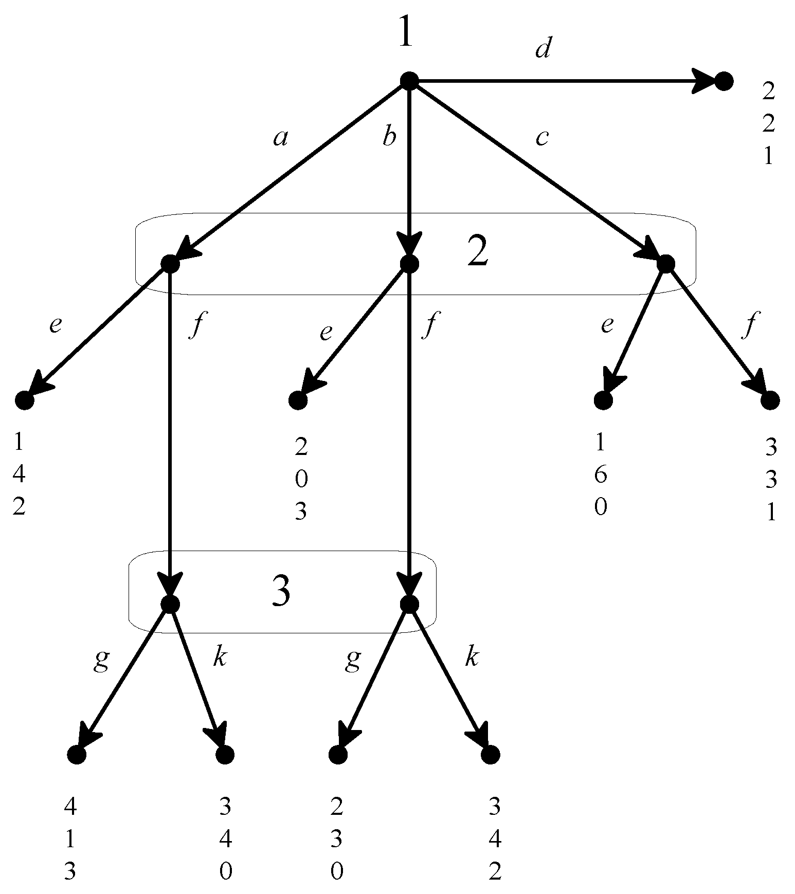
Consider the extensive-form game shown in Figure 17 and the assessment $(\sigma ,\mu )$ where $\sigma =(d,e,g)$ and μ is the following system of beliefs: $\mu \left(a\right)=0,\mu \left(b\right)=\frac{1}{3},\mu \left(c\right)=\frac{2}{3}$ and $\mu \left(af\right)=\mu \left(bf\right)=\frac{1}{2}$. This assessment is AGM-consistent, since it is rationalized by the following plausibility order8:

$$\left(\begin{array}{cc}\mathrm{most}\mathrm{plausible}\hfill & \varnothing ,d\\ \hfill & b,c,be,ce\\ \hfill & a,ae\\ \hfill & af,bf,cf,afg,bfg\\ \mathrm{least}\mathrm{plausible}\hfill & afk,bfk\end{array}\right)$$

(1)

Figure 1. An extensive-form game.

Furthermore $(\sigma ,\mu )$ is sequentially rational9. The property of AGM-consistency imposes restrictions on the support of the behavior strategy σ and on the support of the system of beliefs μ. The following property imposes constraints on how probabilities can be distributed over those supports.

Definition 3.

Given an extensive form, let ≾ be a plausibility order that rationalizes the assessment $(\sigma ,\mu )$. We say that $(\sigma ,\mu )$ is Bayes consistent (or Bayesian) relative to ≾ if, for every equivalence class E of ≾ that contains some decision history h with $\mu \left(h\right)>0$ [that is, $E\cap D_{\mu }^{+}\ne ⌀$, where $D_{\mu }^{+}=\{h\in D:\mu \left(h\right)>0\}$], there exists a probability density function ${\nu }_E:H\to [0,1]$ (recall that H is a finite set) such that:

$\begin{array}{cc}B1.\hfill & {\nu }_E\left(h\right)>0\mathit{if}\mathit{and}\mathit{only}\mathit{if}h\in E\cap D_{\mu }^{+}.\hfill \\ B2.\hfill & \mathit{If}h,h^{\prime }\in E\cap D_{\mu }^{+}\mathit{and}{h}^{\prime }=h{a}_1\dots a_m(\mathit{that}\mathit{is},h\mathit{is}\mathrm{a}\mathit{prefix}of{h}^{\prime })\mathit{then}\hfill \\ & {\nu }_E\left(h^{\prime }\right)={\nu }_E\left(h\right)\times \sigma \left(a_1\right)\times \dots \times \sigma \left(a_m\right).\hfill \\ B3.\hfill & \mathit{If}h\in E\cap D_{\mu }^{+},\mathit{then},\forall h^{\prime }\in I\left(h\right),\mu \left(h^{\prime }\right)={\nu }_E\left(h^{\prime }|I\left(h\right)\right)\stackrel{def}{=}\frac{{\nu }_E\left(h^{\prime }\right)}{{\displaystyle \sum _{h^{\prime \prime }\in I\left(h\right)}}{\nu }_E\left(h^{\prime \prime }\right)}.\hfill \end{array}$

Property $B1$ requires that ${\nu }_E\left(h\right)>0$ if and only if $h\in E$ and $\mu \left(h\right)>0$. Property $B2$ requires ${\nu }_E$ to be consistent with the strategy profile σ in the sense that if $h,h^{\prime }\in E$, $\mu \left(h\right)>0$, $\mu \left(h^{\prime }\right)>0$ and $h^{\prime }=h{a}_1\dots a_m$ then the probability that ${\nu }_E$ assigns to $h^{\prime }$ is equal to the probability that ${\nu }_E$ assigns to h multiplied by the probabilities (according to σ) of the actions that lead from h to $h^{\prime }$10. Property $B3$ requires the system of beliefs μ to satisfy Bayes’ rule in the sense that if $h\in E$ and $\mu \left(h\right)>0$ (so that E is the equivalence class of the most plausible elements of $I\left(h\right)$) then, for every history $h^{\prime }\in I\left(h\right)$, $\mu \left(h^{\prime }\right)$ (the probability assigned to $h^{\prime }$ by μ) coincides with the probability of $h^{\prime }$ conditional on $I\left(h\right)$ using the probability density function ${\nu }_E$11.

Consider again the game of Figure 1, and the assessment $(\sigma ,\mu )$ where $\sigma =(d,e,g)$ and $\mu \left(a\right)=0$$,\mu \left(b\right)=\frac{1}{3},\mu \left(c\right)=\frac{2}{3}$ and $\mu \left(af\right)=\mu \left(bf\right)=\frac{1}{2}$. Let ≾ be the plausibility order (1) given above, which rationalizes $(\sigma ,\mu )$. Then $(\sigma ,\mu )$ is Bayes consistent relative to ≾. In fact, we have that $D_{\mu }^{+}=\{\varnothing ,b,c,af,bf\}$ and the equivalence classes of ≾ that have a non-empty intersection with $D_{\mu }^{+}$ are $E_1=\{\varnothing ,d\}$, $E_2=\{b,c,be,ce\}$ and $E_3=\{af,bf,cf,afg,bfg\}$. Let ${\nu }_{E_1}(\varnothing )=1$, ${\nu }_{E_2}\left(b\right)=\frac{1}{3}$, ${\nu }_{E_2}\left(c\right)=\frac{2}{3}$ and ${\nu }_{E_3}\left(af\right)={\nu }_{E_3}\left(bf\right)=\frac{1}{2}$. Then the three probability density functions ${\nu }_{E_1}$, ${\nu }_{E_2}$ and ${\nu }_{E_3}$ satisfy the properties of Definition 3 and hence $(\sigma ,\mu )$ is Bayes consistent relative to ≾.

Definition 4.

An assessment $(\sigma ,\mu )$ is a perfect Bayesian equilibrium (PBE) if it is sequentially rational, it is rationalized by a plausibility order on the set of histories and is Bayes consistent relative to it.

We saw above that, for the game illustrated in Figure 1, the assessment $(\sigma ,\mu )$ where $\sigma =(d,e,g)$ and $\mu \left(a\right)=0,\mu \left(b\right)=\frac{1}{3},\mu \left(c\right)=\frac{2}{3}$ and $\mu \left(af\right)=\mu \left(bf\right)=\frac{1}{2}$ is sequentially rational, it is rationalized by the plausibility order (1) and is Bayes consistent relative to it. Thus it is a perfect Bayesian equilibrium.

Remark 1.

It is proved in [5] that if $(\sigma ,\mu )$ is a perfect Bayesian equilibrium then σ is a subgame-perfect equilibrium and that every sequential equilibrium is a perfect Bayesian equilibrium. Furthermore, the notion of PBE is a strict refinement of subgame-perfect equilibrium and sequential equilibrium is a strict refinement of PBE.

Next we recall the definition of sequential equilibrium [1]. An assessment $(\sigma ,\mu )$ is KW-consistent (KW stands for ‘Kreps-Wilson’) if there is an infinite sequence $⟨{\sigma }^1,\dots ,{\sigma }^m,\dots ⟩$ of completely mixed behavior strategy profiles such that, letting ${\mu }^m$ be the unique system of beliefs obtained from ${\sigma }^m$ by applying Bayes’ rule12, ${lim}_{m\to \infty }({\sigma }^m,{\mu }^m)=(\sigma ,\mu )$. An assessment $(\sigma ,\mu )$ is a sequential equilibrium if it is KW-consistent and sequentially rational. In [8] it is shown that sequential equilibrium can be characterized as a strengthening of PBE based on two properties: (1) a property of the plausibility order that constrains the supports of the belief system; and (2) a strengthening of the notion of Bayes consistency, that imposes constraints on how the probabilities can be distributed over those supports. The details are given below.

Given a plausibility order ≾ on the finite set of histories H, a function $F:H\to \mathbb{N}$ (where $\mathbb{N}$ denotes the set of non-negative integers) is said to be an ordinal integer-valued representation of ≾ if, for every $h,h^{\prime }\in H$,

$$F\left(h\right)\le F\left(h^{\prime }\right)\mathrm{if}\mathrm{and}\mathrm{only}\mathrm{if}h\precsim h^{\prime }.$$

(2)

Since H is finite, the set of ordinal integer-valued representations is non-empty. A particular ordinal integer-valued representation, which we will call canonical and denote by ρ, is defined as follows.

Definition 5.

Let $H_0=\{h\in H:h\precsim x,\forall x\in H\}$, $H_1=\{h\in H\backslash H_0:h\precsim x,\forall x\in H\backslash H_0\}$ and, in general, for every integer $k\ge 1$, $H_k=\{h\in H\backslash H_0\cup \dots \cup H_{k-1}:h\precsim x,\forall x\in H\backslash H_0\cup \dots \cup H_{k-1}\}$. Thus $H_0$ is the equivalence class of ≾ containing the most plausible histories, $H_1$ is the equivalence class containing the most plausible among the histories left after removing those in $H_0$, etc.13 The canonical ordinal integer-valued representation of ≾, $\rho :H\to \mathbb{N}$, is given by

$$\rho \left(h\right)=k\mathit{if}\mathit{and}\mathit{only}\mathit{if}h\in H_k.$$

(3)

We call $\rho \left(h\right)$ the rank of history $h.$

Instead of an ordinal integer-valued representation of the plausibility order one could seek a cardinal representation which, besides (2), satisfies the following property: if h and $h^{\prime }$ belong to the same information set (that is, $h^{\prime }\in I\left(h\right)$) and $a\in A\left(h\right)$, then

$$F\left(h^{\prime }\right)-F\left(h\right)=F\left(h^{\prime }a\right)-F\left(ha\right).$$

(CM)

If we think of F as measuring the “plausibility distance” between histories, then we can interpret $CM$ as a distance-preserving condition: the plausibility distance between two histories in the same information set is preserved by the addition of the same action.

Definition 6.

A plausibility order ≾ on the set of histories H is choice measurable if it has at least one integer-valued representation that satisfies property $CM$.

For example, the plausibility order (1) is not choice measurable, since any integer-valued representation F of it must be such that $F\left(a\right)-F\left(b\right)>0$ and $F\left(af\right)-F\left(bf\right)=0$.

Let $(\sigma ,\mu )$ be an assessment which is rationalized by a plausibility order ≾. As before, let $D_{\mu }^{+}$ be the set of decision histories to which μ assigns positive probability: $D_{\mu }^{+}=\left\{h\in D:\mu \left(h\right)>0\right\}$. Let ${\mathcal{E}}_{\mu }^{+}$ be the set of equivalence classes of ≾ that have a non-empty intersection with $D_{\mu }^{+}$. Clearly ${\mathcal{E}}_{\mu }^{+}$ is a non-empty, finite set. Suppose that $(\sigma ,\mu )$ is Bayesian relative to ≾ and let ${\left\{{\nu }_E\right\}}_{E\in {\mathcal{E}}_{\mu }^{+}}$ be a collection of probability density functions that satisfy the properties of Definition 3. We call a probability density function $\nu :D\to (0,1]$ a full-support common prior of ${\left\{{\nu }_E\right\}}_{E\in {\mathcal{E}}_{\mu }^{+}}$ if, for every $E\in {\mathcal{E}}_{\mu }^{+}$, ${\nu }_E(·)=\nu (·|E\cap D_{\mu }^{+})$, that is, for all $h\in E\cap D_{\mu }^{+}$, ${\nu }_E\left(h\right)=\frac{\nu \left(h\right)}{{\displaystyle \sum _{h^{\prime }\in E\cap D_{\mu }^{+}}}\nu \left(h^{\prime }\right)}$. Note that a full support common prior assigns positive probability to all decision histories, not only to those in $D_{\mu }^{+}$.

Definition 7.

Consider an extensive form. Let $(\sigma ,\mu )$ be an assessment which is rationalized by the plausibility order ≾ and is Bayesian relative to it and let ${\left\{{\nu }_E\right\}}_{E\in {\mathcal{E}}_{\mu }^{+}}$ be a collection of probability density functions that satisfy the properties of Definition 3. We say that $(\sigma ,\mu )$ is uniformly Bayesian relative to ≾ if there exists a full-support common prior $\nu :D\to (0,1]$ of ${\left\{{\nu }_E\right\}}_{E\in {\mathcal{E}}_{\mu }^{+}}$ that satisfies the following properties.

$\begin{array}{cc}UB1.\hfill & \mathit{If}a\in A\left(h\right)\mathit{and}ha\in D,\mathit{then}\hfill \\ & \left(i\right)\nu \left(ha\right)\le \nu \left(h\right)\mathit{and},\left(ii\right)\mathit{if}\sigma \left(a\right)>0\mathit{then}\nu \left(ha\right)=\nu \left(h\right)\times \sigma \left(a\right).\hfill \\ UB2.\hfill & \mathit{If}a\in A\left(h\right),h\mathit{and}{h}^{\prime }\mathit{belong}\mathit{to}\mathit{the}\mathit{same}\mathit{information}\mathit{set}\mathit{and}ha,h^{\prime }a\in D\hfill \\ & \mathit{then}\frac{\nu \left(h\right)}{\nu \left(h^{\prime }\right)}=\frac{\nu \left(ha\right)}{\nu \left(h^{\prime }a\right)}.\hfill \end{array}$

We call such a function ν auniform full-support common prior of ${\left\{{\nu }_E\right\}}_{E\in {\mathcal{E}}_{\mu }^{+}}$.

$UB1$ requires that the common prior ν be consistent with the strategy profile σ, in the sense that if $\sigma \left(a\right)>0$ then $\nu \left(ha\right)=\nu \left(h\right)\times \sigma \left(a\right)$ (thus extending Property $B2$ of Definition 3 from $D_{\mu }^{+}$ to D). $UB2$ requires that the relative probability, according to the common prior ν, of any two histories that belong to the same information set remain unchanged by the addition of the same action.

It is shown in [8] that choice measurability and uniform Bayesian consistency are independent properties. The following proposition is proved in [8].

Proposition 1.

(I) and (II) below are equivalent:

(I) 

($\sigma ,\mu$) is a perfect Bayesian equilibrium which is rationalized by a choice

measurable plausibility order and is uniformly Bayesian relative to it.

(II) 

($\sigma ,\mu$) is a sequential equilibrium.

3. Exploring the Gap between PBE and Sequential Equilibrium

The notion of perfect Bayesian equilibrium (Definition 4) incorporates—through the property of AGM-consistency—a belief revision policy which can be interpreted either as the epistemic state of an external observer14 or as a belief revision policy which is shared by all the players15. For example, the perfect Bayesian equilibrium considered in Section 2 for the game of Figure 1, namely $\sigma =(d,e,g)$ and $\mu \left(a\right)=0,\mu \left(b\right)=\frac{1}{3},\mu \left(c\right)=\frac{2}{3}$, $\mu \left(af\right)=\mu \left(bf\right)=\frac{1}{2}$ reflects the following belief revision policy: the initial beliefs are that Player 1 will play d; conditional on learning that Player 1 did not play d, the observer would become convinced that Player 1 played either b or c (that is, she would judge a to be less plausible than b and she would consider c to be as plausible as b) and would expect Player 2 to play e; upon learning that (Player 1 did not play d and) Player 2 played f, the observer would become convinced that Player 1 played either a or b, hence judging $af$ to be as plausible as $bf$, thereby modifying her earlier judgment that a was less plausible than b. Although such a belief revision policy does not violate the rationality constraints introduced in [7], it does involve a belief change that is not “minimal”or “conservative”. Such “non-minimal” belief changes can be ruled out by imposing the following restriction on the plausibility order: if h and $h^{\prime }$ belong to the same information set (that is, $h^{\prime }\in I\left(h\right)$) and a is an action available at h($a\in A\left(h\right)$), then

$$h\precsim h^{\prime }\mathrm{if}\mathrm{and}\mathrm{only}\mathrm{if}ha\precsim h^{\prime }a.$$

(IND₁)

$IN{D}_1$ says that if h is deemed to be at least as plausible as $h^{\prime }$ then the addition of any available action a must preserve this judgment, in the sense that $ha$ must be deemed to be at least as plausible as $h^{\prime }a$, and vice versa; it can also be viewed as an “independence” condition, in the sense that observation of a new action cannot lead to a change in the relative plausibility of previous histories16. Any plausibility order that rationalizes the assessment $\sigma =(d,e,g)$ and $\mu \left(a\right)=0,\mu \left(b\right)=\frac{1}{3},\mu \left(c\right)=\frac{2}{3}$, $\mu \left(af\right)=\mu \left(bf\right)=\frac{1}{2}$ for the game of Figure 1 must violate $IN{D}_1$ (since $b\prec a$ while $bf\sim af$).

We can obtain a strengthening of the notion of perfect Bayesian equilibrium (Definition 4) by (1) adding property $IN{D}_1$; and (2) strengthening Bayes consistency (Definition 3) to uniform Bayesian consistency (Definition 7).

Definition 8.

Given an extensive-form game, an assessment (σ,μ) is a weakly independent perfect Bayesian equilibrium if it is sequentially rational, it is rationalized by a plausibility order that satisfies $IN{D}_1$ and is uniformly Bayesian relative to that plausibility order.

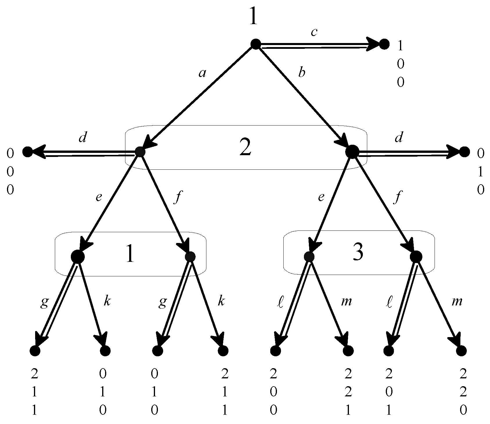
As an example of a weakly independent PBE consider the game of Figure 2 and the assessment (σ,μ) where $\sigma =(c,d,g,\ell )$ (highlighted by double edges in Figure 2) and $\mu \left(b\right)=\mu \left(ae\right)=\mu \left(bf\right)=1$ (thus $\mu \left(a\right)=\mu \left(af\right)=\mu \left(be\right)=0$) (the decision histories x such that $\mu \left(x\right)>0$ are shown as black nodes and the decision histories x such that $\mu \left(x\right)=0$ are shown as gray nodes)). This assessment is sequentially rational and is rationalized by the following plausibility order:

$$\left(\begin{array}{cc}\mathrm{most}\mathrm{plausible}\hfill & \varnothing ,c\\ \hfill & b,bd\\ \hfill & a,ad\\ \hfill & bf,bf\ell \\ \hfill & be,be\ell \\ \hfill & ae,aeg\\ \hfill & af,afg\\ \hfill & bfm\\ \hfill & bem\\ \hfill & aek\\ \mathrm{least}\mathrm{plausible}\hfill & afk\end{array}\right)$$

(4)

Figure 2.

It is straightforward to check that plausibility order (4) satisfies $IN{D}_1$17. To see that (σ,μ) is uniformly Bayesian relative to plausibility order (4), note that $D_{\mu }^{+}=\{\varnothing ,b,ae,bf\}$ and thus the only equivalence classes that have a non-empty intersection with $D_{\mu }^{+}$ are $E_1=\{\varnothing ,c\}$, $E_2=\{b,bd\}$, $E_3=\{ae,aeg\}$ and $E_4=\{bf,bf\ell \}$. Letting ${\nu }_{E_1}(\varnothing )=1$, ${\nu }_{E_2}\left(b\right)=1$, ${\nu }_{E_3}\left(ae\right)=1$ and ${\nu }_{E_4}\left(bf\right)=1$, this collection of probability distributions satisfies the Properties of Definition 3. Let ν be the uniform distribution over the set of decision histories $D=\{\varnothing ,a,b,ae,af,be,bf\}$ (thus $\nu \left(h\right)=\frac{1}{7}$ for every $h\in D$). Then ν is a full support common prior of the collection ${\left\{{\nu }_{E_i}\right\}}_{i\in \{1,2,3,4\}}$ and satisfies Properties $UB1$ and $UB2$ of Definition 7.

Note, however, that (σ,μ) is not a sequential equilibrium. This can be established by showing that (σ,μ) is not KW-consistent; however, we will show it by appealing to the following lemma (proved in Appendix A) which highlights a property that will motivate a further restriction on belief revision (property $IN{D}_2$ below).

Lemma 1.

Let ≾ be a plausibility order over the set H of histories of an extensive-form game and let $F:H\to \mathbb{N}$ be an integer-valued representation of ≾ (that is, for all $h,h^{\prime }\in H$, $F\left(h\right)\le F\left(h^{\prime }\right)$ if and only if $h\precsim h^{\prime }$). Then the following are equivalent:

(A) 

F satisfies Property $CM$ (Definition 6)

(B) 

F satisfies the following property: for all $h,h^{\prime }\in H$ and $a,b\in A\left(h\right)$, if $h^{\prime }\in I\left(h\right)$ then

$$F\left(hb\right)-F\left(ha\right)=F\left(h^{\prime }b\right)-F\left(h^{\prime }a\right)$$

(CM^′)

.

Using Lemma 1 we can prove that the assessment (σ,μ) where $\sigma =(c,d,g,\ell )$ and $\mu \left(b\right)=\mu \left(ae\right)=\mu \left(bf\right)=1$, for the game of Figure 2, is not a sequential equilibrium. By Proposition 1 it will be sufficient to show that (σ,μ) cannot be rationalized by a choice measurable plausibility order (Definition 6). Let ≾ be a plausibility order that rationalizes (σ,μ) and let F be an integer-valued representation of ≾. Then, by ($P2)$ of Definition 2, it must be that $ae\prec af$ (because $\mu \left(ae\right)>0$ and $\mu \left(af\right)=0$) and $bf\prec be$ (because $\mu \left(bf\right)>0$ and $\mu \left(be\right)=0$); thus $F\left(ae\right)-F\left(af\right)<0$ and $F\left(be\right)-F\left(bf\right)>0$, so that F violates property $C{M}^{\prime }$; hence, by Lemma 1, F violates property $CM$ and thus ≾ is not choice measurable.

The ordinal counterpart to Property $C{M}^{\prime }$ is Property $IN{D}_2$ below, which can be viewed as another “independence” condition: it says that if action a is implicitly judged to be at least as plausible as action b, conditional on history h (that is, $ha\precsim hb$), then the same judgment must be made conditional on any other history that belongs to the same information set as h: if $h^{\prime }\in I\left(h\right)$ and $a,b\in A\left(h\right)$, then

$$ha\precsim hb\mathrm{if}\mathrm{and}\mathrm{only}\mathrm{if}{h}^{\prime }a\precsim h^{\prime }b.$$

(IND₂)

Note that Properties $IN{D}_1$ and $IN{D}_2$ are independent. An example of a plausibility order that violates $IN{D}_1$ but satisfies $IN{D}_2$ is plausibility order (1) for the game of Figure 1: $IN{D}_1$ is violated because $b\prec a$ but $bf\sim af$ and $IN{D}_2$ is satisfied because at every non-singleton information set there are only two choices, one of which is plausibility preserving and the other is not. An example of a plausibility order that satisfies $IN{D}_1$ but violates $IN{D}_2$ is plausibility order (4) for the game of Figure 218. Adding Property $IN{D}_2$ to the properties given in Definition 8 we obtain a refinement of the notion of weakly independent perfect Bayesian equilibrium.

Definition 9.

Given an extensive-form game, an assessment (σ,μ) is a strongly independent perfect Bayesian equilibrium if it is sequentially rational, it is rationalized by a plausibility order that satisfies Properties $IN{D}_1$ and $IN{D}_2$, and is uniformly Bayesian relative to that plausibility order.

The following proposition states that the notions of weakly/strongly independent PBE identify two (nested) solution concepts that lie strictly in the gap between PBE and sequential equilibrium. The proof of the first part of Proposition 2 is given in Appendix A, while the example of Figure 3 establishes the second part.

Figure 3.

Proposition 2.

Consider an extensive-form game and an assessment (σ,μ). If (σ,μ) is a sequential equilibrium then it is a strongly independent perfect Bayesian equilibrium (PBE). Furthermore, there are games where there is a strongly independent PBE which is not a sequential equilibrium.

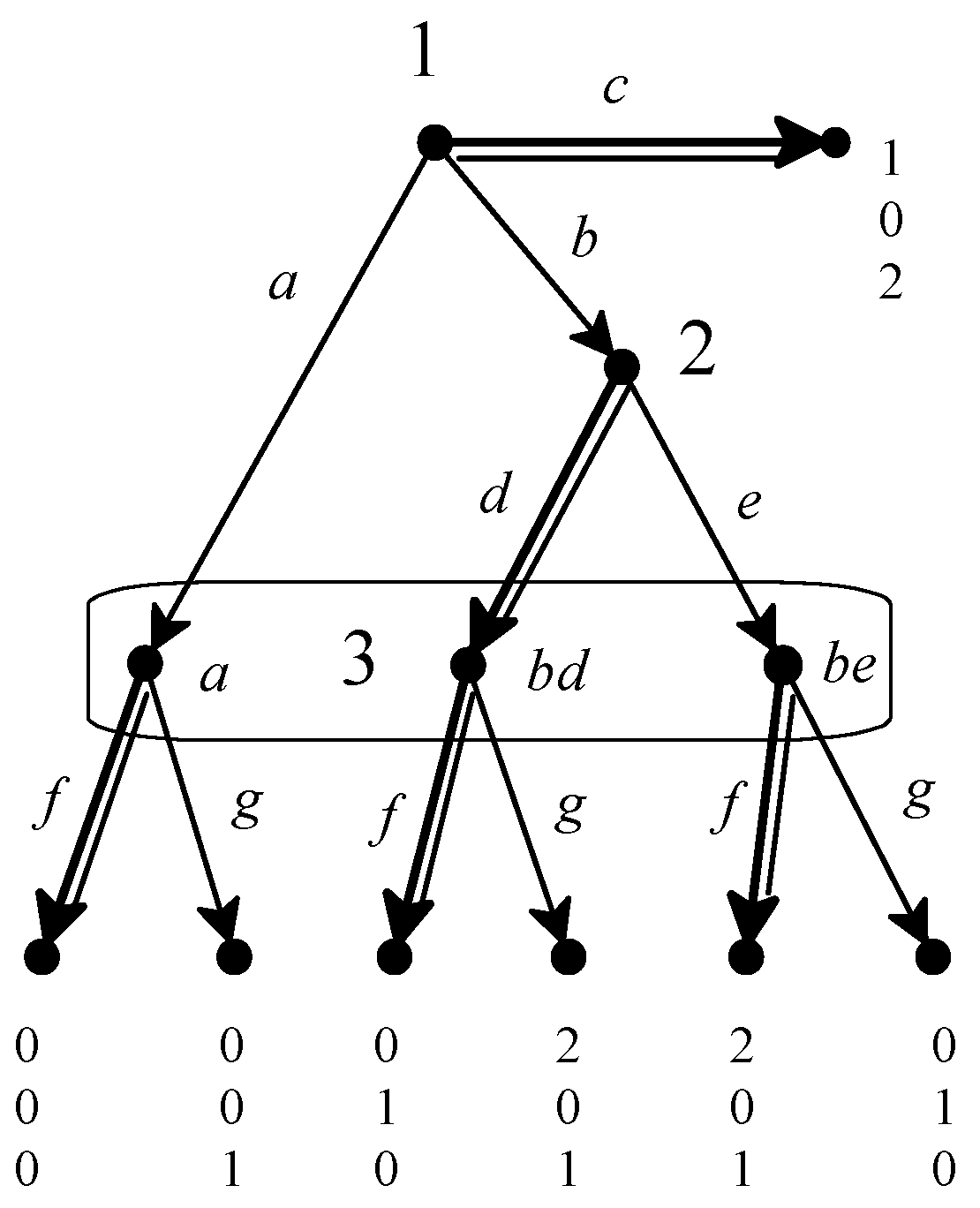
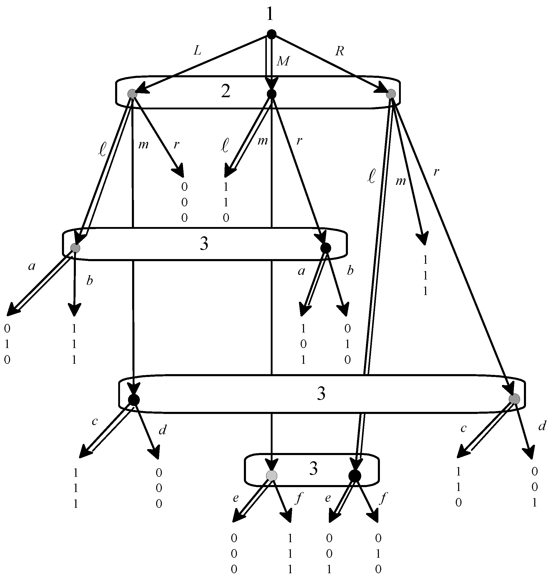
To see that the notion of strongly independent PBE is weaker than sequential equilibrium, consider the game of Figure 3 (which is based on an example discussed in [12,13,14]) and the assessment $(\sigma ,\mu )$ where $\sigma =(M,\ell ,a,c,e)$ (highlighted by double edges), $\mu \left(x\right)=1$ for $x\in \{\varnothing ,M,Mr,Lm,R\ell \}$ and $\mu \left(x\right)=0$ for every other decision history x (the decision histories x such that $\mu \left(x\right)>0$ are shown as black nodes and the decision histories x such that $\mu \left(x\right)=0$ are shown as gray nodes). This assessment is rationalized by the following plausibility order:

$$\left(\begin{array}{cc}\mathrm{most}\mathrm{plausible}& \varnothing ,M,M\ell \\ & R,R\ell ,R\ell e\\ & Mm,Mme\\ & Mr,Mra\\ & L,L\ell ,L\ell a\\ & Rm\\ & Lm,Lmc\\ & Rr,Rrc\\ & Lr\\ & R\ell f\\ & Mmf\\ & Lmd\\ & Rrd\\ & Mrb\\ \mathrm{least}\mathrm{plausible}& L\ell b\end{array}\right)$$

(5)

It is straightforward to check that plausibility order (5) satisfies Properties $IN{D}_1$19 and $IN{D}_2$20. Furthermore (σ,μ) is trivially uniformly Bayesian relative to plausibility order (5)21. Thus (σ,μ) is a strongly independent PBE. Next we show that (σ,μ) is not a sequential equilibrium, by appealing to Proposition 1 and showing that any plausibility order that rationalizes (σ,μ) is not choice measurable22. Let ≾ be a plausibility order that rationalizes $(\sigma ,\mu )$; then it must satisfy the following properties:

• $Lm\prec Rr$ (because they belong to the same information set and $\mu \left(Lm\right)>0$ while $\mu \left(Rr\right)=0$). Thus if F is any integer-valued representation of ≾ it must be that

  $$F\left(Lm\right)<F\left(Rr\right).$$

  (6)
• $Mr\prec L\ell \sim L$ (because $Mr$ and $L\ell$ belong to the same information set and $\mu \left(Mr\right)>0$ while $\mu \left(L\ell \right)=0$; furthermore, ℓ is a plausibility-preserving action since $\sigma \left(\ell \right)>0$). Thus if F is any integer-valued representation of ≾ it must be that

  $$F\left(Mr\right)<F\left(L\right).$$

  (7)
• $R\sim R\ell \prec Mm$ (because ℓ is a plausibility-preserving action, $R\ell$ and $Mm$ belong to the same information set and $\mu \left(R\ell \right)>0$ while $\mu \left(Mm\right)=0$). Thus if F is any integer-valued representation of ≾ it must be that

  $$F\left(R\right)<F\left(Mm\right).$$

  (8)

Suppose that ≾ is choice measurable and let F be an integer-valued representation of it that satisfies Property $CM$. From (6) and (7) we get that

$$F\left(Lm\right)-F\left(L\right)<F\left(Rr\right)-F\left(Mr\right)$$

(9)

and by Property $CM$ it must be that

$$F\left(Rr\right)-F\left(Mr\right)=F\left(R\right)-F\left(M\right).$$

(10)

It follows from (9) and (10) that

$$F\left(Lm\right)-F\left(L\right)<F\left(R\right)-F\left(M\right).$$

(11)

Subtracting $F\left(M\right)$ from both sides of (8) we obtain

$$F\left(R\right)-F\left(M\right)<F\left(Mm\right)-F\left(M\right).$$

(12)

It follows from (11) and (12) that $F\left(Lm\right)-F\left(L\right)<F\left(Mm\right)-F\left(M\right)$, which can be written as $F\left(M\right)-F\left(L\right)<F\left(Mm\right)-F\left(Lm\right)$, yielding a contradiction, because Property $CM$ requires that $F\left(M\right)-F\left(L\right)=F\left(Mm\right)-F\left(Lm\right)$.

Are the notions of weakly/strongly independent PBE “better” or “more natural” than the basic notion of PBE? This issue will be discussed briefly in Section 6.

4. How to Determine if a Plausibility Order Is Choice Measurable

In this section we provide a method for determining if a plausibility order is choice measurable. More generally, we provide a necessary and sufficient condition that applies not only to plausibility orders over sets of histories in a game but to a more general class of structures.

Let S be an arbitrary finite set and let ≾ be a total pre-order on S. Let ${S\backslash }_{\sim }$ be the set of ≾-equivalence classes of S. If $s\in S,$ the equivalence class of s is denoted by $\left[s\right]=\{t\in S:s\sim t\}$ (where, as before, $s\sim t$ is a short-hand for “$s\precsim t$ and $t\precsim s$”); thus ${S\backslash }_{\sim }=\{\left[s\right]:s\in S\}$. Let ≐ be an equivalence relation on ${S\backslash }_{\sim }{\times S\backslash }_{\sim }$. The interpretation of $(\left[s_1\right],\left[s_2\right])\doteq (\left[t_1\right],\left[t_2\right])$ is that the distance between the equivalence classes $\left[s_1\right]$ and $\left[s_2\right]$ is required to be equal to the distance between the equivalence classes $\left[t_1\right]$ and $\left[t_2\right]$.

Remark 2.

In the special case of a plausibility order ≾ on the set of histories H of a game, we shall be interested in the following equivalence relation ≐ on ${H\backslash }_{\sim }{\times H\backslash }_{\sim }$, which is meant to capture property $CM$ above: if $E_1$, $E_2$, $F_1$ and $F_2$ are equivalence classes of ≾ then $(E_1,E_2)\doteq (F_1,F_2)$ if and only if there exist two decision histories $h,h^{\prime }\in H$ that belong to the same information set [$h^{\prime }\in I\left(h\right)$] and a non-plausibility-preserving action $a\in A\left(h\right)$ such that $h\in E_1,h^{\prime }\in E_2,ha\in F_1$ and $h^{\prime }a\in F_2$ (or $ha\in E_1,h^{\prime }a\in E_2,h\in F_1$ and $h^{\prime }\in F_2$).

The general problem that we are addressing is the following.

Problem 1.

Given a pair $(\precsim ,\doteq )$, where ≾ is a total pre-order on a finite set S and ≐ is an equivalence relation on the set of pairs of equivalence classes of ≾, determine whether there exists a function $F:S\to \mathbb{N}$ such that, for all $s,t,x,y\in S$, (1) $F\left(s\right)\le F\left(t\right)$ if and only if $s\precsim t$ and (2) if $\left(\right[s],[t\left]\right)\doteq \left(\right[x],[y\left]\right)$, with $s\prec t$ and $x\prec y$, then $F\left(t\right)-F\left(s\right)=F\left(y\right)-F\left(x\right)$.

Instead of expressing the equivalence relation ≐ in terms of pairs of elements of ${S\backslash }_{\sim }$, we shall express it in terms of pairs of numbers $(j,k)$ obtained by using the canonical ordinal representation ρ of ≾23. That is, if $s_1,s_2,t_1,t_2\in S$ and $(\left[s_1\right],\left[s_2\right])\doteq (\left[t_1\right],\left[t_2\right])$ then we shall write this as $\left(\rho \left(s_1\right),\rho \left(s_2\right)\right)\doteq \left(\rho \left(t_1\right),\rho \left(t_2\right)\right)$. For example, let $S=\{a,b,c,d,e,f,g,h,\ell ,m\}$ and let ≾ be as shown in (13) below, together with the corresponding canonical representation ρ24:

$$\left(\begin{array}{cc}\precsim :& \rho :\\ a& 0\\ b,c& 1\\ d& 2\\ e& 3\\ f,g& 4\\ h,\ell & 5\\ m& 6\end{array}\right)$$

(13)

If the equivalence relation ≐ contains the following pairs25:

$$\begin{array}{c}\left(\right[a],[b\left]\right)\doteq \left(\right[h],[m\left]\right)\\ \left(\right[a],[b\left]\right)\doteq \left(\right[e],[f\left]\right)\\ \left(\right[a],[d\left]\right)\doteq \left(\right[f],[m\left]\right)\\ \left(\right[b],[e\left]\right)\doteq \left(\right[e],[f\left]\right)\\ \left(\right[b],[e\left]\right)\doteq \left(\right[f],[m\left]\right)\end{array}\mathrm{then}\mathrm{we}\mathrm{express}\mathrm{them}(\mathrm{using}\rho )\mathrm{as}\begin{array}{c}(0,1)\doteq (5,6)\\ (0,1)\doteq (3,4)\\ (0,2)\doteq (4,6)\\ (1,3)\doteq (3,4)\\ (1,3)\doteq (4,6)\end{array}$$

(14)

A bag (or multiset) is a generalization of the notion of set in which members are allowed to appear more than once. An example of a bag is $\left\{1,2,2,3,4,4,5,6\right\}$. Given two bags $B_1$ and $B_2$ their union, denoted by $B_1⋓B_2$, is the bag that contains those elements that occur in either $B_1$ or $B_2$ and, furthermore, the number of times that each element occurs in $B_1⋓B_2$ is equal to the number of times it occurs in $B_1$ plus the number of times it occurs in $B_2$. For instance, if $B_1=\left\{1,2,2,3,4,4,5,6\right\}$ and $B_2=\left\{2,3,6,6\right\}$ then $B_1⋓B_2=\left\{1,2,2,2,3,3,4,4,5,6,6,6\right\}$. We say that $B_1$ is a proper sub-bag of $B_2$, denoted by $B_1⊏B_2,$ if $B_1\ne B_2$ and each element that occurs in $B_1$ occurs also, and at least as many times, in $B_2.$ For example, $\left\{1,2,4,4,5,6\right\}⊏\left\{1,1,2,4,4,5,5,6\right\}.$

Given a pair $(i,j)$ with $i<j$, we associate with it the set $B_{(i,j)}=\{i+1,i+2,\dots ,j\}$. For example, $B_{(2,5)}=\{3,4,5\}.$ Given a set of pairs $P=\{(i_1,j_1),(i_2,j_2),\dots ,(i_m,j_m)\}$ (with $i_k<j_k,$ for every $k=1,\dots ,m$) we associate with it the bag $B_P=B_{(i_1,j_1)}⋓B_{(i_2,j_2)}⋓\dots ⋓B_{(i_m,j_m)}$. For example, if $P=\left\{\right(0,2),(1,4),(2,5\left)\right\}$ then $B_P=\{1,2\}⋓\{2,3,4\}⋓\{3,4,5\}=\{1,2,2,3,3,4,4,5\}.$

Definition 10.

For every element of ≐, expressed (using the canonical representation ρ) as $(i,j)\doteq (k,\ell )$ (with $i<j$ and $k<\ell$), the equation corresponding to it is $x_{i+1}+x_{i+2}+\dots +x_j=x_{k+1}+x_{k+2}+\dots +x_{\ell }$. By the system of equations corresponding to ≐ we mean the set of all such equations26.

For example, consider the total pre-order given in (13) and the following equivalence relation ≐ (expressed in terms of ρ and omitting the reflexive pairs):

$$\left\{(0,3)\doteq (2,4),(2,4)\doteq (0,3),(2,4)\doteq (3,5),(3,5)\doteq (2,4),(0,3)\doteq (3,5),(3,5)\doteq (0,3)\right\}$$

Then the corresponding system of equations is given by:

$$\begin{array}{c}\hfill x_1+x_2+x_3=x_3+x_4\hfill \\ x_3+x_4=x_1+x_2+x_3\\ x_3+x_4=x_4+x_5\\ x_4+x_5=x_3+x_4\\ x_1+x_2+x_3=x_4+x_5\\ x_4+x_5=x_1+x_2+x_3\end{array}$$

(15)

We are now ready to state the solution to Problem 1. The proof is given in Appendix A.

Proposition 3.

Given a pair $(\precsim ,\doteq )$, where ≾ is a total pre-order on a finite set S and ≐ is an equivalence relation on the set of pairs of equivalence classes of ≾, (A), (B) and (C) below are equivalent.

(A) 

There is a function $F:S\to \mathbb{N}$ such that, for all $s,t,x,y\in S$, (1) $F\left(s\right)\le F\left(t\right)$ if and only if $s\precsim t$; and (2) if $\left(\right[s],[t\left]\right)\doteq \left(\right[x],[y\left]\right)$, with $s\prec t$ and $x\prec y$, then $F\left(t\right)-F\left(s\right)=F\left(y\right)-F\left(x\right)$,

(B) 

The system of equations corresponding to ≐ (Definition 10) has a solution consisting of positive integers.

(C) 

There is no sequence $⟨\left((i_1,j_1)\doteq (k_1,{\ell }_1)\right),\dots ,\left((i_m,j_m)\doteq (k_m,{\ell }_m)\right)⟩$ in ≐ (expressed in terms of the canonical representation ρ of ≾ ) such that $B_{left}⊏B_{right}$ where $B_{left}=B_{(i_1,j_1)}⋓\dots ⋓B_{(i_m,j_m)}$ and $B_{right}=B_{(k_1,{\ell }_1)}⋓\dots ⋓B_{(k_m,{\ell }_m)}$.

As an application of Proposition 3 consider again the game of Figure 3 and plausibility order (5) which rationalizes the assessment $\sigma =(M,\ell ,a,c,e)$, $\mu \left(x\right)=1$ for $x\in \{\varnothing ,M,Mr,Lm,R\ell \}$ and $\mu \left(x\right)=0$ for every other decision history x; the order is reproduced below together with the canonical integer-valued representation ρ:

$$\left(\begin{array}{ccc}& \precsim :& \rho :\\ \mathrm{most}\mathrm{plausible}& \varnothing ,M,M\ell & 0\\ & R,R\ell ,R\ell e& 1\\ & Mm,Mme& 2\\ & Mr,Mra& 3\\ & L,L\ell ,L\ell a& 4\\ & Rm& 5\\ & Lm,Lmc& 6\\ & Rr,Rrc& 7\\ & Lr& 8\\ & R\ell f& 9\\ & Mmf& 10\\ & Lmd& 11\\ & Rrd& 12\\ & Mrb& 13\\ \mathrm{least}\mathrm{plausible}& L\ell b& 14\end{array}\right)$$

(16)

By Remark 2, two elements of ≐ are $\left(\right[M],[R\left]\right)\doteq \left(\right[Mr],[Rr\left]\right)$ and $\left(\right[Mm],[Lm\left]\right)\doteq \left(\right[M],[L\left]\right)$, which—expressed in terms of the canonical ordinal representation ρ—can be written as

$$(0,1)\doteq (3,7)$$

$$(2,6)\doteq (0,4)$$

Then $B_{left}=\left\{1\right\}⋓\{3,4,5,6\}=\{1,3,4,5,6\}$ and $B_{right}=\{4,5,6,7)⋓\{1,2,3,4\}=\{1,2,3,4,4,5,6,7\}$. Thus, since $B_{left}⊏B_{right}$, by Part (C) of Proposition 3 ≾ is not choice measurable.

As a further application of Proposition 3 consider the total pre-order ≾ given in (13) together with the subset of the equivalence relation ≐ given in (14). Then there is no cardinal representation of ≾ that satisfies the constraints expressed by ≐, because of Part (C) of the above proposition and the following sequence27:

$$⟨\left((0,1)\doteq (3,4)\right),\left((1,3)\doteq (4,6)\right),\left((3,4)\doteq (1,3)\right),\left((4,6)\doteq (0,2)\right)⟩$$

where $B_{left}=\left\{1\right\}⋓\{2,3\}⋓\left\{4\right\}⋓\{5,6\}=\{1,2,3,4,5,6\}⊏B_{right}=\left\{4\right\}⋓\{5,6\}⋓\{2,3\}⋓\{1,2\}=\{1,2,2,3,4,5,6\}.$

In fact, the above sequence corresponds to the following system of equations:

$$\begin{array}{ccc}{x}_1=x_4& \mathrm{corresponding}\mathrm{to}& (0,1)\doteq (3,4)\\ x_2+x_3=x_5+x_6& \mathrm{corresponding}\mathrm{to}& (1,3)\doteq (4,6)\\ x_4=x_2+x_3& \mathrm{corresponding}\mathrm{to}& (3,4)\doteq (1,3)\\ x_5+x_6=x_1+x_2& \mathrm{corresponding}\mathrm{to}& (4,6)\doteq (0,2)\end{array}$$

Adding the four equations we get $x_1+x_2+x_3+x_4+x_5+x_6=x_1+2x_2+x_3+x_4+x_5+x_6$ which simplifies to $0=x_2$, which is incompatible with a positive solution.

Remark 3.

In [15] an algorithm is provided for determining whether a system of linear equations has a positive solution and for calculating such a solution if one exists. Furthermore, if the coefficients of the equations are integers and a positive solution exists, then the algorithm yields a solution consisting of positive integers.

5. Related Literature

As noted in Section 1, the quest in the literature for a “simple” solution concept intermediate between subgame-perfect equilibrium and sequential equilibrium has produced several attempts to provide a general definition of perfect Bayesian equilibrium.

In [16] a notion of perfect Bayesian equilibrium was provided for a small subset of extensive-form games (namely the class of multi-stage games with observed actions and independent types), but extending that notion to arbitrary games proved to be problematic28.

In [14] a notion of perfect Bayesian equilibrium is provided that can be applied to general extensive-form games (although it was defined only for games without chance moves); however, the proposed definition is in terms of a more complex object, namely a “tree-extended assessment” $(\nu ,\sigma ,\mu )$ where ν is a conditional probability system on the set of terminal nodes. The main idea underlying the notion of perfect Bayesian equilibrium proposed in [14] is what the author calls “strategic independence”: when forming beliefs, the strategic choices of different players should be regarded as independent events.

Several more recent contributions [5,17,18] have re-addressed the issue of providing a definition of perfect Bayesian equilibrium that applies to general extensive-form games. Since [5] has been the focus of this paper, here we shall briefly discuss [17,18]. In [17] the notion of “simple perfect Bayesian equilibrium” is introduced and it is shown to lie strictly between subgame-perfect equilibrium and sequential equilibrium. This notion is based on an extension of the definition of sub-tree, called “quasi sub-tree”, which consists of an information set I together with all the histories that are successors of histories in I (that is, ${\mathsf{\Gamma }}_I$ is a quasi-subtree that starts at I if $h^{\prime }\in {\mathsf{\Gamma }}_I$ if and only if there exists an $h\in I$ such that h is a prefix of $h^{\prime }$). A quasi sub-tree ${\mathsf{\Gamma }}_I$ is called regular if it satisfies the following property: if $h\in {\mathsf{\Gamma }}_I$ and $h^{\prime }\in I\left(h\right)$ then $h^{\prime }\in {\mathsf{\Gamma }}_I$ (that is, every information set that has a non-empty intersection with ${\mathsf{\Gamma }}_I$ is entirely included in ${\mathsf{\Gamma }}_I$). 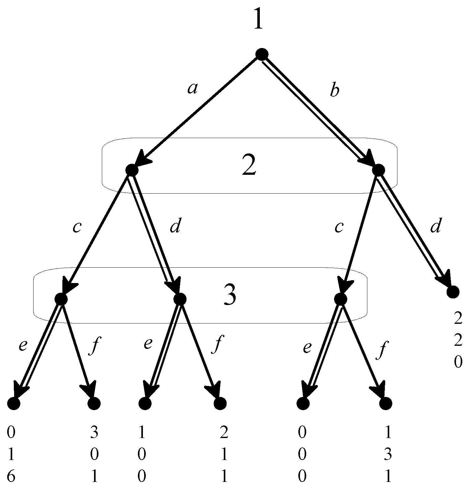An information set I is called regular if the quasi-subtree that starts at I is regular. For example, in the game of Figure 4, the singleton information set $\left\{b\right\}$ of Player 2 is not regular. An assessment ($\sigma ,\mu$) is defined to be a “simple perfect Bayesian equilibrium” if it is sequentially rational and, for every regular quasi-subtree ${\mathsf{\Gamma }}_I$, Bayes’ rule is satisfied at every information set that is reached with positive probability by σ in ${\mathsf{\Gamma }}_I$ (in other words, if the restriction of ($\sigma ,\mu$) to every regular quasi-subtree is a weak sequential equilibrium of the quasi-subtree). This notion of perfect Bayesian equilibrium is weaker than the notion considered in this paper (Definition 4). For example, in the game of Figure 4, the pure-strategy profile $\sigma =(c,d,f)$ (highlighted by double edges), together with the system of beliefs $\mu \left(a\right)=\mu \left(bd\right)=0,\mu \left(be\right)=1$, is a simple perfect Bayesian equilibrium, while (as shown in [5]) there is no system of beliefs ${\mu }^{\prime }$ such that $(\sigma ,{\mu }^{\prime })$ is a perfect Bayesian equilibrium. A fortiori, the notion of simple perfect Bayesian equilibrium is weaker than the refinements of PBE discussed in the Section 3.

Figure 4.

In [18], the author proposes a definition of perfect Bayesian equilibrium which is framed not in terms of assessments but in terms of “appraisals”. Each player is assumed to have a (possibly artificial) information set representing the beginning of the game and an appraisal for player i is a map that associates with every information set of player i a probability distribution over the set of pure-strategy profiles that reach that information set. Thus an appraisal for player i captures, for every information set of hers, her conjecture about how the information set was reached and what will happen from this point in the game. An appraisal system is defined to be “plainly consistent” if, whenever an information set of player i has a product structure (each information set is identified with the set of pure-strategy profiles that reach that information set), the player’s appraisal at that information set satisfies independence29. A strategy profile σ is defined to be a perfect Bayesian equilibrium if there is a plainly consistent appraisal system P that satisfies sequential rationality and is such that at their “initial” information sets all the players assign probability 1 to σ; in [18] (p. 15), the author summarizes the notion of PBE as being based on “a simple foundation: sequential rationality and preservation of independence and Bayesian updating where applicable” (that is, on subsets of strategy profiles that have the appropriate product structure and independence property). Despite the fact that the notion of PBE suggested in [18] incorporates a notion of independence, it can be weaker than the notion of PBE discussed in Section 2 (Definition 4) and thus, a fortiori, weaker than the notion of weakly independent PBE (Definition 8, Section 3). This can be seen from the game of Figure 5, which essentially reproduces an example given in [18]. The strategy profile $\sigma =(b,d,e)$ (highlighted by double edges), together with any system of beliefs μ such that $\mu \left(ac\right)>0$ cannot be a PBE according to Definition 4 (Section 2). In fact, since $\sigma \left(d\right)>0$ while $\sigma \left(c\right)=0$, any plausibility order that rationalizes $(\sigma ,\mu )$ must be such that $a\sim ad\prec ac$, which implies that $\mu \left(ac\right)=0$ (because $ac$ cannot be most plausible in the set $\{ac,ad,bc\}$). On the other hand, σ can be a PBE according to the definition given in [18] (p. 15), since the information set of Player 3 does not have a product structure so that Player 3 is not able to separate the actions of Players 1 and 2. For example, consider the appraisal system P where, initially, all the players assign probability 1 to σ and, at his information set, Player 2 assigns probability 1 to the strategy profile $(b,e)$ of Players 1 and 3 and, at her information set, Player 3 assigns probability $\frac{1}{3}$ to each of the strategy profiles $(a,c),(a,d)$ and $(b,c)$ of Players 1 and 2. Then P is plainly consistent and sequentially rational, so that σ is a PBE as defined in [18].

Figure 5.

Thus, a fortiori, the notion of perfect Bayesian equilibrium given in [18] can be weaker than the notions of weakly/strongly independent PBE introduced in Section 3.

6. Conclusions

Besides sequential rationality, the notion of perfect Bayesian equilibrium (Definition 4) introduced in [5] is based on two elements: (1) rationalizability of the assessment by a plausibility order (Definition 2); and (2) the notion of Bayesian consistency relative to the plausibility order. The first property identifies the set of decision histories that can be assigned positive conditional probability by the system of beliefs, while the second property imposes constraints on how conditional probabilities can be distributed over that set in order to guarantee “Bayesian updating as long as possible”30. In [8] it was shown that by strengthening these two conditions one obtains a “limit free” characterization of sequential equilibrium. The strengthening of the first condition is that the plausibility order that rationalizes the given assessment be choice measurable, that it, that there be a cardinal representation of it (which can be interpreted as measuring the plausibility distance between histories in a way that is preserved by the addition of a common action). The strengthening of the second condition imposes “uniform consistency” on the conditional probability density functions on the equivalence classes of the plausibility order, by requiring that there be a full-support common prior that preserves the relative probabilities of two decision histories in the same information set when a common action is added. There is a “substantial” gap between the notion of PBE and that of sequential equilibrium. In this paper we identified two solution concepts that lie in this gap. The first notion, weakly independent PBE (Definition 8), is obtained by adding a restriction on the belief revision policy encoded in the plausibility order that rationalizes the given assessment (together with strengthening Bayes consistency to uniform Bayes consistency). This restriction says that observation of a new action at an information set should not alter the relative plausibility of any two histories in that information set (condition $IN{D}_1$); it can be interpreted as an “independence” or “conservative” principle, in the sense that observation of a new action should not lead to a reversal of judgment of plausibility concerning past histories. The second notion, strongly independent PBE (Definition 9), is obtained by adding to the first notion a further restriction, according to which the implicit plausibility ranking of two actions available at the same information set should be independent of the history at which the actions are taken.

A further contribution of this paper has been to provide a method for determining if a plausibility order is choice measurable, which is one of the two conditions that, together, are necessary and sufficient for a PBE to be a sequential equilibrium.

This paper highlights the need to conceptualize refinements of subgame-perfect equilibrium in extensive form games in terms of principles of belief revision. Through the notion of plausibility order and AGM-consistency we have appealed to the principles of belief revision that underlie the so-called AGM theory [7]. However, in a dynamic game, beliefs typically need to be revised several times in a sequence as new information sets are reached. Thus the relevant notion of belief revision is iterated belief revision. There is an extensive literature on the topic of iterated belief revision (see, for example, [19,20,21,22] and the special issue of the Journal of Philosophical Logic, Vol. 40 (2), April 2011). An exploration of different solution concepts in the gap between PBE and sequential equilibrium, based on different principles of iterated belief revision, seems to be a promising area of research.