Strategic Voting in Heterogeneous Electorates: An Experimental Study

Abstract

We study strategic voting in a setting where voters choose from three options and Condorcet cycles may occur. We introduce in the electorate heterogeneity in preference intensity by allowing voters to differ in the extent to which they value the three options. Three information conditions are tested: uninformed, in which voters know only their own preference ordering and the own benefits from each option; aggregate information, in which in addition they know the aggregate realized distribution of the preference orderings and full information, in which they also know how the relative importance attributed to the options are distributed within the electorate. As a general result, heterogeneity seems to decrease the level of strategic voting in our experiment compared to the homogenous preference case that we study in a companion paper. Both theoretically and empirically (with data collected in a laboratory experiment), the main comparative static results obtained for the homogenous case carry over to the present setting with preference heterogeneity. Moreover, information about the realized aggregate distribution of preferences seems to be the element that best explains observed differences in voting behavior. Additional information about the realized distribution of preference intensity does not yield significant further changes.

1. Introduction

Voting is a means of collective decision making that is observed at all levels of society, ranging from family decisions on where to spend the day to large-scale nationwide elections. Using plurality rule to jointly make a decision comes naturally. For example, if subjects in a laboratory experiment are asked to make a group decision and no decision rule is specified, they naturally arrive at plurality rule as a means to make a group decision [1]. Plurality rule has the appealing intuition that it provides a straightforward way to reach the decision that “is preferred by most”. This intuition fails, however, if (some) people do not vote for their most preferred outcome but, instead, vote strategically for a less preferred option. The reason to do so may be to avoid even less-preferred outcomes from receiving most votes. Strategic voting is an important phenomenon that has been studied theoretically, empirically and experimentally [2,3,4,5,6].

In a previous companion study ([7]; henceforth TS11) we investigated strategic voting in an environment where Condorcet cycles may occur. In particular, we were interested in the effects of information about the distribution of preferences across voters. That study also varied the relative importance of the second preferred option. Our results showed high levels of strategic voting. An important limitation of the previous study is that it assumes that electorates are homogenous in the relative importance attributed to the second option. This means that every voter attributes the same utility to the second most preferred option (and also the same for the most and least preferred options). Of course, the particular option that a voter ranks as second, varied across the electorate. We then compared electorates where voters attributed relatively high value to the second option (i.e., for every voter, there was a good second best) to electorates where the second option was relatively bad (voters had a lot to lose if their most preferred option was not chosen).

In this paper, we consider the complementary case of electorates with preferences that are heterogeneous in the relative importance attributed to the second most preferred option. For ease of presentation, we refer to these as “heterogeneous preferences”.1 In a general sense, heterogeneity in preferences has been shown to be important in explaining economic and political behavior including social preferences [8,9], risk and time preferences [10], the perception of national economic conditions [11] and electoral choices [12]. Note that this literature provides little guidance as to what to expect for heterogeneity as we apply it, however. The interaction between strategic voting and preference heterogeneity has to the best of our knowledge not been considered before. To obtain insights into its effects, we study preference heterogeneity both theoretically and in a controlled laboratory environment. TS11 (pp. 3–4) provide a discussion of the merits of laboratory experimentation in this research area. Two important advantages of laboratory control are that it (i) provides direct and unbiased information about voters’ (induced) preference orderings over the alternatives; and (ii) allows for a systematic study of the causes and consequences of strategic voting in an environment where preference orderings are clearly defined and known to the experimenter.

As an illustration of why heterogeneity may matter, consider a voter, A, who supports the a-priori least popular alternative (i.e., the alternative with least support if everyone votes sincerely). Assume that A attributes high value to the intermediate option. In the heterogeneous case, the other players with the same preference ordering as A attribute, on average, lower value to the second option than in the homogenous case (because—contrary to the homogenous case—some attribute low value to it). Hence, the probability that these other players will vote strategically is lower in the heterogeneous case. In turn, this reduces for A the expected value of voting strategically. In other words, preference heterogeneity will reduce strategic voting by supporters of the least popular alternative.2

Our theory and experiment build on the model developed in TS11. They are set in an environment characterized by plurality rule and mandatory voting. With homogeneous preferences, our theoretical results (supported by experimental data) predicted strategic voting, with its extent increasing in the availability of information about others’ preferences, and in the relative importance given to one’s second best candidate. It is possible, however, that such results do not carry over to an environment with heterogeneous preferences. This is the main question we will pursue here. In particular, we investigate the impact of heterogeneity within and across information settings.

As a general result, heterogeneity seems to decrease the level of strategic voting in our experiment. A possible explanation is that when the complexity of the environment increases, voters are more likely to replace rather complicated strategies by more simple heuristics, such as voting sincerely [13,14]. Moreover, our previously found comparative static results for information are robust to preference heterogeneity. Note that information has two components in this context: (i) the aggregate distribution of voters with respect to the preference ordering; and (ii) the intensity of preferences within each group. Under homogeneous preferences, when (i) is known, then (ii) is also known. Expanding the original model to allow for heterogeneous preferences makes it possible to inform voters about the aggregate distribution of preference ordering (i) without giving information on the intensity of preferences (ii). This allows us to isolate the effects of the two types of information. Our experimental data show that information about the aggregate distribution of preferences is the more important element in explaining observed differences across treatments in voting behavior.

This remainder of this paper is structured as follows. The next section presents the model, its theoretical analysis and derives testable behavioral predictions. Section 3 introduces the experimental design and procedures and is followed by the results in Section 4. Section 5 concludes.

2. The Model

The model extends the specification in TS11. Each voter i = 1, …, N has a strict preference ordering over three alternatives, denoted by A, B, C and is required to cast exactly one vote for an alternative. Voters are assumed to maximize (expected) utility, which is determined by the elected alternative. Plurality rule determines the winner, with ties broken by an equal probability random draw. The utility of each voter is set according to the rank of the elected alternative. If her preferred, intermediate or least preferred alternative is elected she receives , or respectively. Note that (contrary to our companion paper) these utilities may vary across individuals. Normalizing by setting = 10 and = 1, each voter’s preferences are characterized by , the utility she attributes to the intermediate option.

Before each election, all voters’ preferences and value of are determined randomly, independently across voters and voting periods. While the own preference ordering and value are revealed to the voter by nature at the beginning of each period, the extent of information about the electorate’s preferences and values are also variables in the model. An electorate is therefore, characterized by the number of voters, probability distributions of preference orderings and values, and by the amount of pre-election information.

Because we are not interested in specific characteristics of the distinct options, we focus on a game in which every voter has an a priori symmetric problem regardless of her preference ordering. We therefore restrict the possible preferences to {(A, B, C); (B, C, A); (C, A, B)}, in which the listed order represents the preference ordering. Preference orderings are randomly chosen from this set. Note that these preferences typically form a Condorcet cycle potentially giving rise to strategic behavior.

We consider two values for the intermediate option . A low value = 3 indicates a low relative importance of one’s second best option compared to the best option and, thus a high intensity of preference. A high value = 8 reflects a high importance and low intensity of preference. With homogeneous preferences as in TS11, in a given electorate all voters have either a low or high value. In the heterogeneous setting studied here, each voter has either a low or high value with equal probability.

Finally, three distinct levels of information will be of interest: (i) in an uninformed setting, aside from their own values, voters know only the prior probability distributions of preferences and ;3 (ii) in an aggregate information setting, voters also know the ex-post realized distribution of preference orderings for the election concerned, but not the realized distribution of ; (iii) in a full information setting voters also know the ex-post realized distribution of within each preference ordering.

2.1. Theoretical Analysis

A Quantal Response Equilibrium model ([15])—henceforth QRE—is used to analyze the game. We opt for QRE because it has been shown to more accurately predict individual behavior in various political choice problems than Nash equilibrium does [15,16,17]). For example, it can account for the (seemingly irrational) high turnout rates in large-scale national elections, where Nash predicts unrealistically low turnout ([18]). QRE has the intuitive advantage that it allows for boundedly rational behavior while at the same time assuming that the deviation from rationality declines as the stakes become larger.

We start with the uninformed case; i.e., a voter knows only the electorate size, the prior probability distribution of preference orderings, the prior distribution of the intensity of preferences and the own preference ordering and intensity. With the latter information, the voter can update the probability distributions using Bayes’ rule and use this to calculate the probability of being pivotal given others’ strategies. Then, she can compute the expected payoff differences between voting for her best, second best or for the least preferred alternative.4 The QRE Model captures the pivotal probabilities since in its computation only the differences in expected payoff matter, rendering all non-pivotal situations as irrelevant (for details, see Appendix A in TS11).

In line with the previous literature (e.g., [19,20,21]) we define a sincere vote as a vote for one’s preferred option and a strategic vote as a vote for one’s second best option. We consider the QRE for electorates with 12 voters, which corresponds to the numbers in our experiments. Figure 1 shows the probabilities of voting strategically and sincerely on the principal branch of the Multinomial Logit Correspondence (MLC)5 for the game without information. For the noise parameter in QRE (denoted by µ) we will concentrate on the range µ ∈ [0.4; 0.8]. This is the range estimated to fit previous laboratory data on voter participation ([16]).

Figure 1. Multinomial Logit Correspondence (Uninformed Setting).

Figure 1. Multinomial Logit Correspondence (Uninformed Setting).

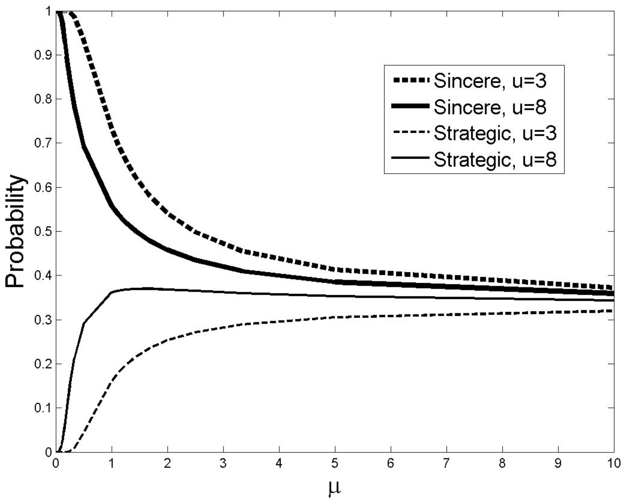Notes. Lines show the principal branch of the MLC for high ( = 8) and low ( = 3) values of the intermediate option, for the 12-voter case.

The figure shows that as µ decreases (corresponding to a decreasing influence of noise in the decision), behavior converges for each voter type to a Bayes-Nash Equilibrium in which all voters vote sincerely. Therefore, a fully rational analysis predicts no difference in behavior across different utilities attributed to the intermediate option. In contrast, when behavior is noisy (µ > 0), the equilibrium probability of a strategic vote is higher for voters with a high value for the intermediate option.6 This predicted (equilibrium) behavior of voters in the heterogeneous setting is precisely the same as we found for the homogenous case in our companion paper (see Figure 1A in TS11). This follows from the symmetry of the game: the equal probabilities of orderings interacts with the equal probabilities of intensity of preferences such that, with only prior information, a player’s better response depends only on her own intensity of preferences. Two behavioral predictions follow. First, a voter is more likely to vote strategically when her intermediate option value is high. Second, theory predicts no difference in behavior when comparing uninformed voters under homogeneous versus heterogeneous settings.

Consider next the settings with information. Voters know the aggregate distribution of preferences and may or may not know the realized distribution of the intensity of preferences. For an illustration, consider the cases that can serve as direct comparison for the a priori expected situation. With aggregate information this is the equal split on the preference orderings (i.e., four voters with each preference ordering). With full information this corresponds to the equal split on preference orderings and on intensity of preferences (i.e., two voters of each group have = 3 and two have = 8). As information increases, the uncertainty about the situation is reduced. Figure 2 depicts these two scenarios.

First notice that with information and high importance of the intermediate option the limiting QRE does not comprise sincere voting. The equilibrium converges to a mixed strategy profile in which a strategic vote happens with 24% and 21% respectively for the aggregate and full information cases. Second, notice how similar the two cases are. This seems to indicate that the aggregate information about preferences, which is the common element, is the key to understanding behavior in the model. Of course, the cases depicted in Figure 2 are just one of the possible realizations. Figure 3 depicts the average behavior across all possible realizations (weighted by the probability of a realization occurring).

Qualitatively, the results are similar to those in Figure 2. Notice that now in all cases the limiting average Nash equilibrium is a mixed profile. Specifically, for the low (high) intermediate values it converges to 23% (32%) for the aggregate and 23% (29%) for the full information case. Three behavioral predictions can be made. First, as in the uninformed case, the probability of a strategic vote is increasing in the importance given to the second best option. Second, a comparison with the homogenous case in TS11 (in particular, Figure 3) shows that—as in the uninformed case—controlling for the intensity of preferences, there is no effect of heterogeneity on average behavior. Third, if preference orderings are known, information about other’s intensities of preferences does not affect strategic behavior. Comparing Figure 1 and Figure 3 suggests one additional behavioral prediction, namely that more strategic voting is expected with information than without.

Figure 2. Multinomial Logit Correspondence (Informed Settings).

Figure 2. Multinomial Logit Correspondence (Informed Settings).

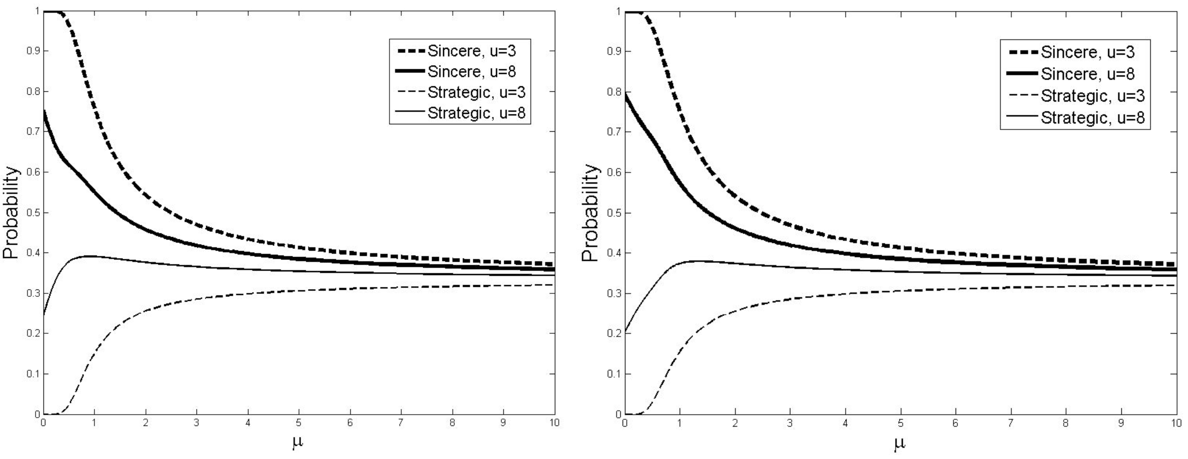
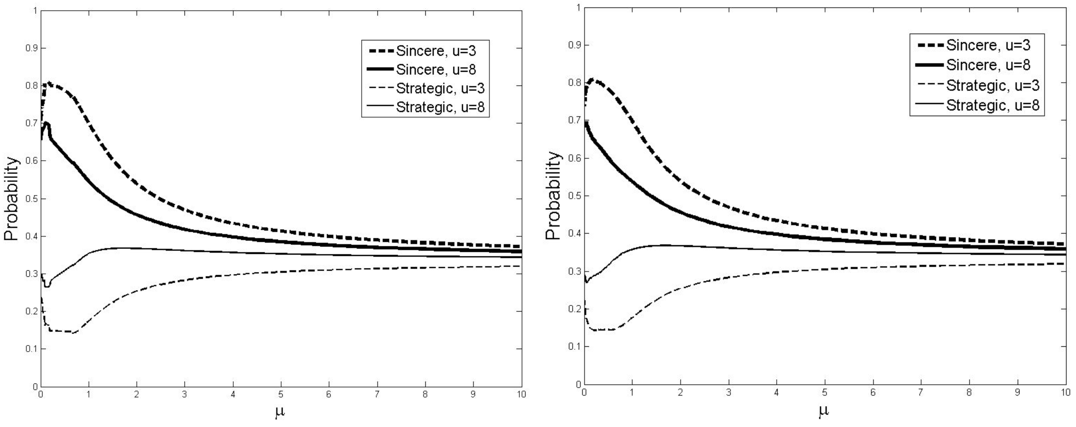
Notes. Lines show the principal branch of the MLC for high ( = 8) and low ( = 3) values of the intermediate option, varying in the extent of information available. For each of the preference orderings, there are four voters. In the left panel voters know the realized aggregate distribution of preference orderings (i.e., how many people have the ordering ABC, how many have BCA and hoe many have CAB), but they only know the distribution of intensity of preferences. In the right panel voters also know the realized intensities. In both cases there are four voters with each of the preference orderings. In the right panel, two voters attribute high value to the intermediate option and two attribute low value.

Figure 3. Average Multinomial Logit Correspondence (Informed Settings).

Figure 3. Average Multinomial Logit Correspondence (Informed Settings).

Notes. Lines show the weighted average (across all preference configurations) of the principal branch of the MLC for high for high ( = 8) and low ( = 3) values of the intermediate option, varying in the extent of information available. In the left panel voters know the realized aggregate distribution of preference orderings, but only the distribution of intensity of preferences. In the right panel voters also know the distribution of intensity of preferences. The average is across all possible combinations of preference orderings, weighted by the probabilities with which they occur.

With information voters know the realized distribution of preferences. As a consequence, they know how many voters share their preferences and how this compares to the number of voters with the other two preference orderings. We define “Rank-Types” according to how a voter’s most preferred candidate then ranks. “Rank 1^st” have the highest preference for the candidate with the largest sincere support; “Rank 2nd” (“Rank 3rd”) have the second (lowest) sincere support.7 Figure 4 shows, for the informed settings, the probability of a strategic vote with voters grouped by Rank-Type and intensity of preferences. It includes the homogeneous cases for completeness (this graph is not given in TS11)8. Rank 1st voters are not included, because they predominantly vote sincerely, in equilibrium.

Figure 4. Strategic Voting by Rank-Type.

Figure 4. Strategic Voting by Rank-Type.

Notes. Lines show the weighted average of the principal branch of the MLC, across information treatments, including the (full information) homogeneous case from TS11 for completeness. Panels distinguish among the possible combinations of Rank-Type and value of the intermediate option (as indicated below the panel). The average is across all possible combinations of preference orderings, weighted by the probabilities with which they occur. Cases where groups are tied for Rank 2nd are not included in the graph.

First notice that when grouping by Rank-Type, the probability of a strategic vote is still increasing in the value of the intermediate option (with the exception of the comparative statics for Rank 2nd under homogeneous preferences). Next, notice that as the literature suggests9, Rank 3rd voters are more likely to cast a strategic vote. Distinct behavior, however, is predicted when comparing across information settings, keeping constant the Rank-Type and intensity of preference (i.e., within panel). For Rank 3rd voters and high value of the intermediate option the introduction of heterogeneity reduces the likelihood of a strategic vote. This is in line with intuition, since the attractiveness of a strategic vote (i.e., its expected value) is related to the expected behavior of other voters with the same preference ordering. If these players attribute, on average, lower value to the second option, their probability of a strategic vote is smaller, which in turn should reduce the equilibrium behavior of voters with a high value. This comparative static is reversed when considering Rank 2nd voters with high value. This may be an equilibrium response to the reactions by Rank 3rd voters to the heterogeneity. Finally, for voters with a low value of the intermediate option the effect of heterogeneity is exactly the opposite of their high value counterpart, but the effect is small.

2. Behavioral Predictions

The experiments to be described below study strategic voting and its interaction with information and preference heterogeneity. Summarizing the analysis from the previous sub-section, the following behavioral predictions will be tested:

(1)

The probability of strategic voting is increasing in the value attributed to the intermediate option, for all information settings (Figure 1, Figure 3 and Figure 4).

(2)

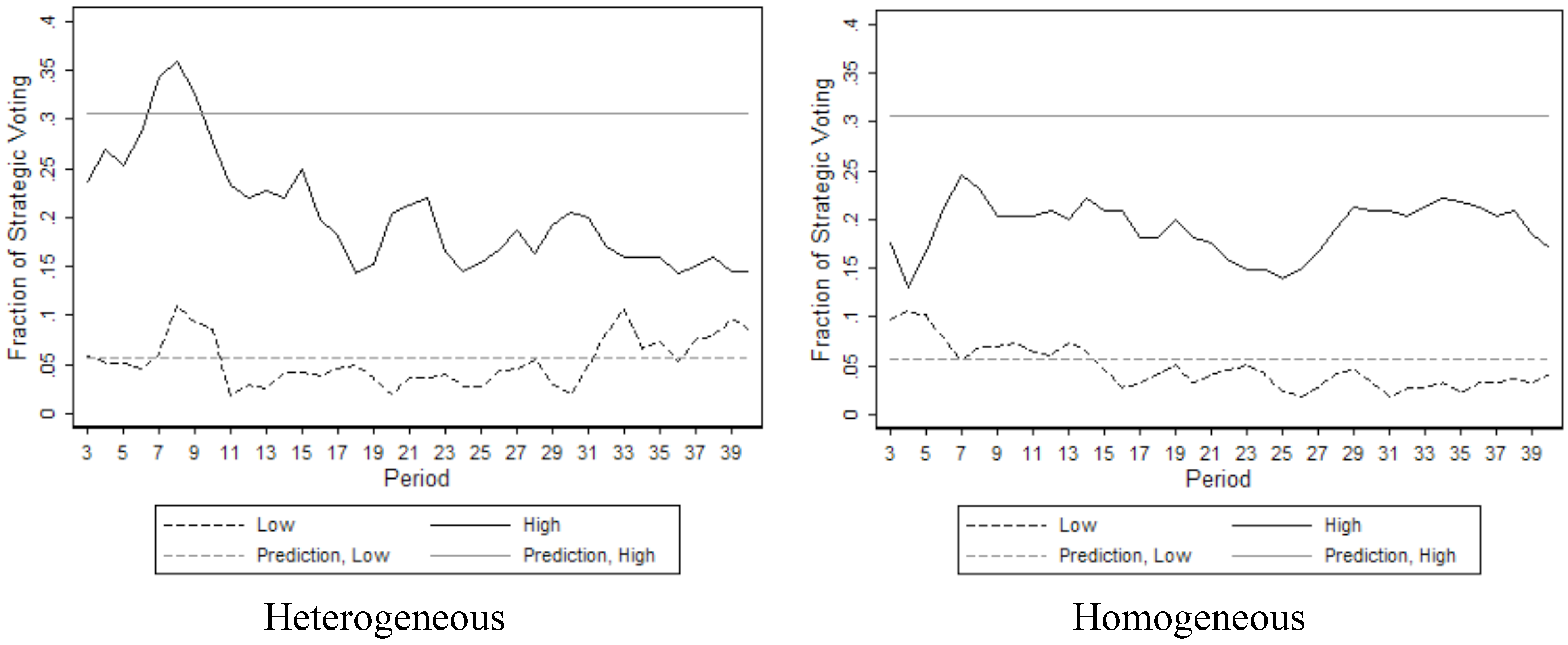
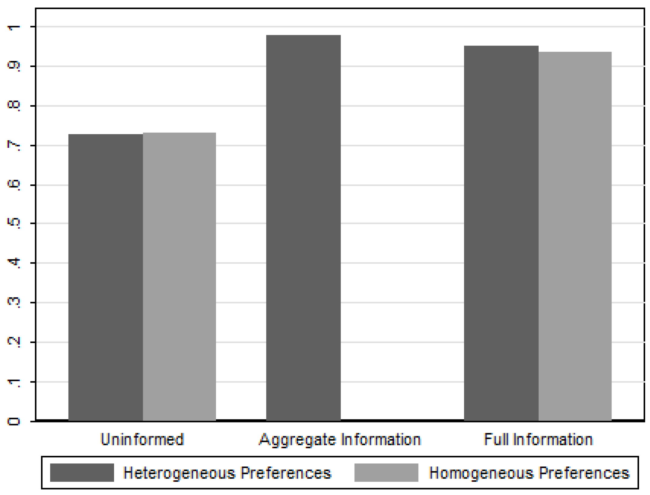
Without information, there is no effect of heterogeneity on the probability of strategic voting (Figure 1 in comparison to TS11).

(3)

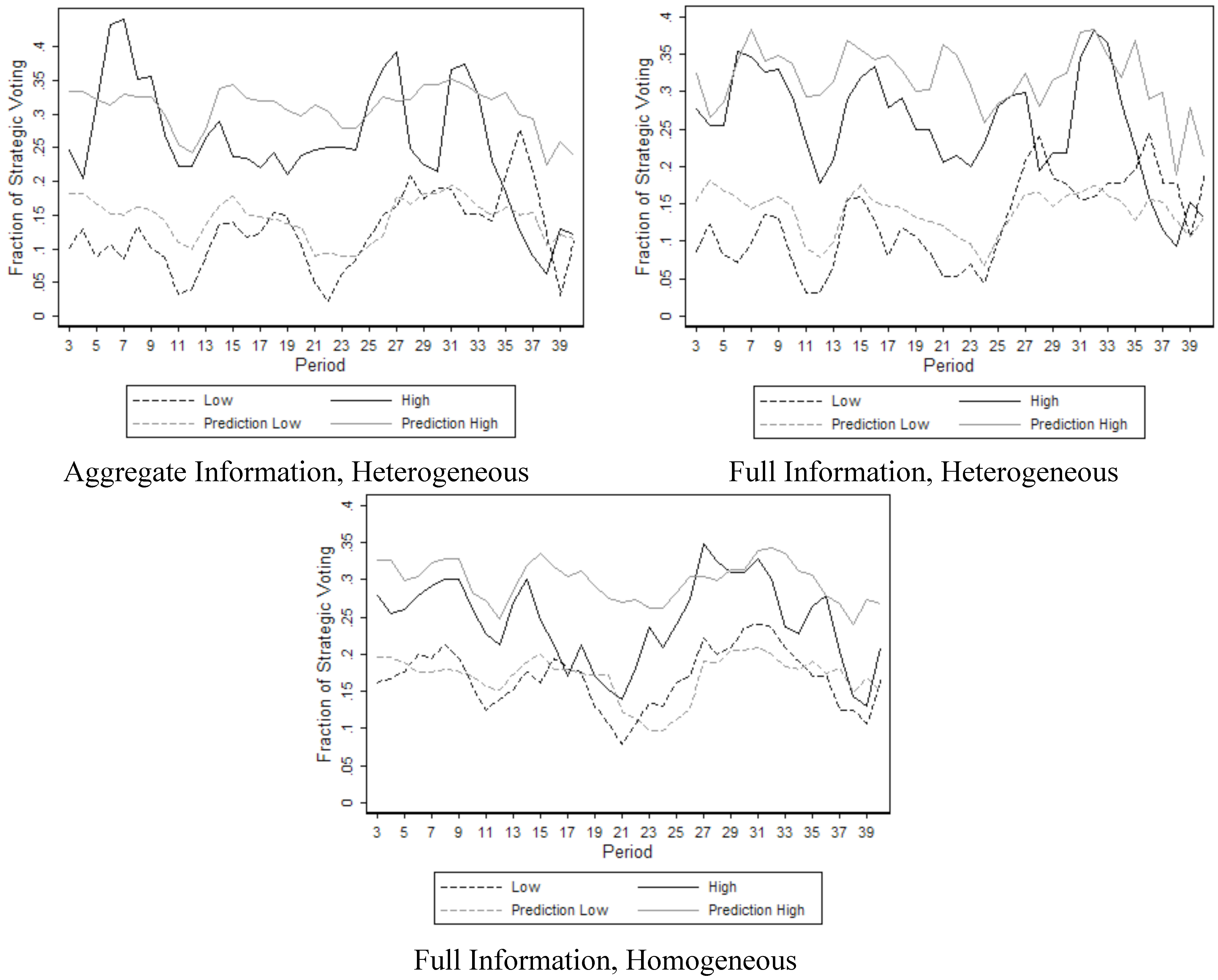
With information, there is no effect of heterogeneity on average behavior (Figure 3 in comparison to TS11).

(4)

Information about other’s intensities of preferences does not affect strategic behavior if preference orderings are known (Figure 3).

(5)

The probability of strategic voting is higher with information than without (Figure 1 vs. Figure 3).

(6)

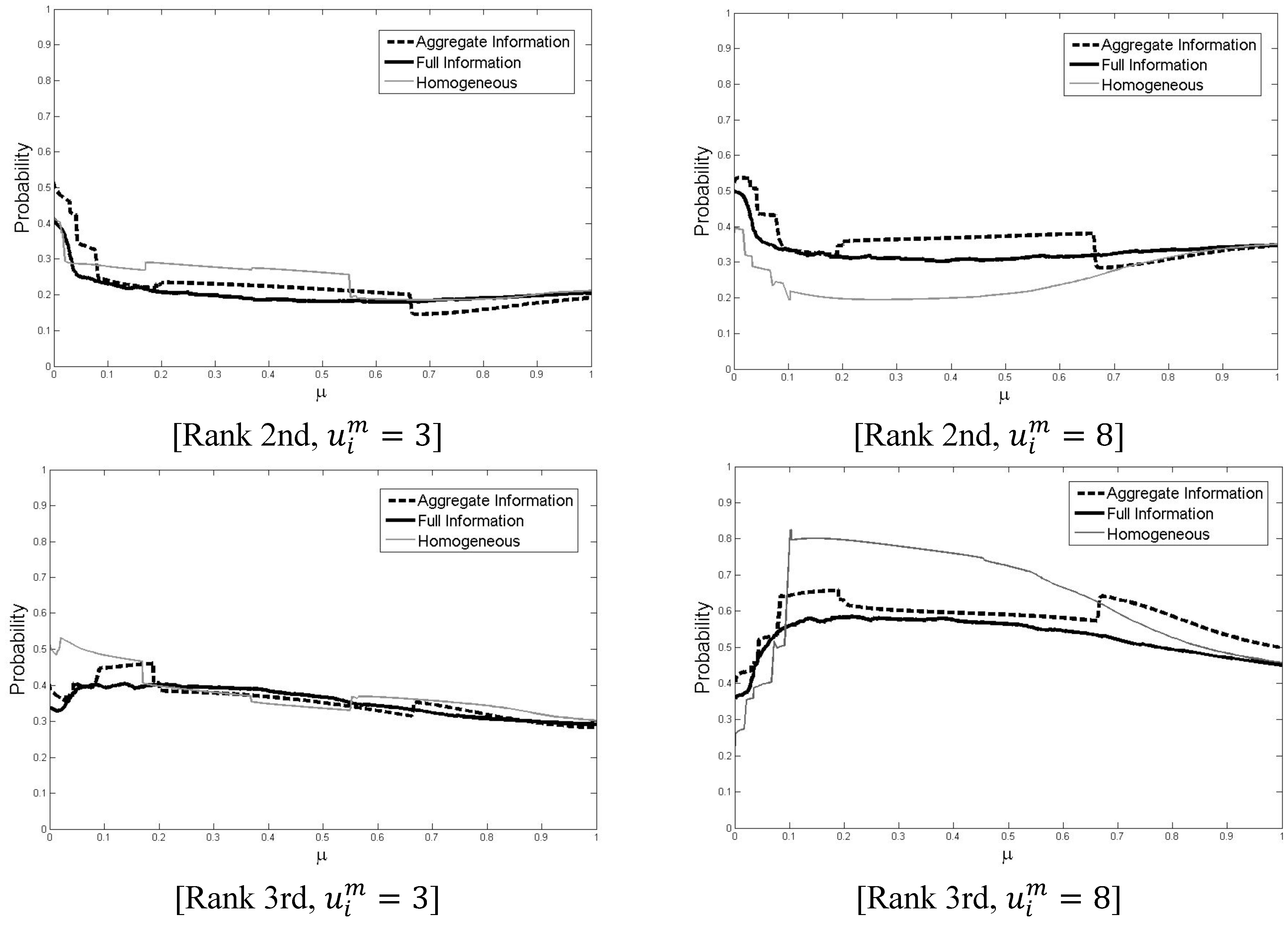
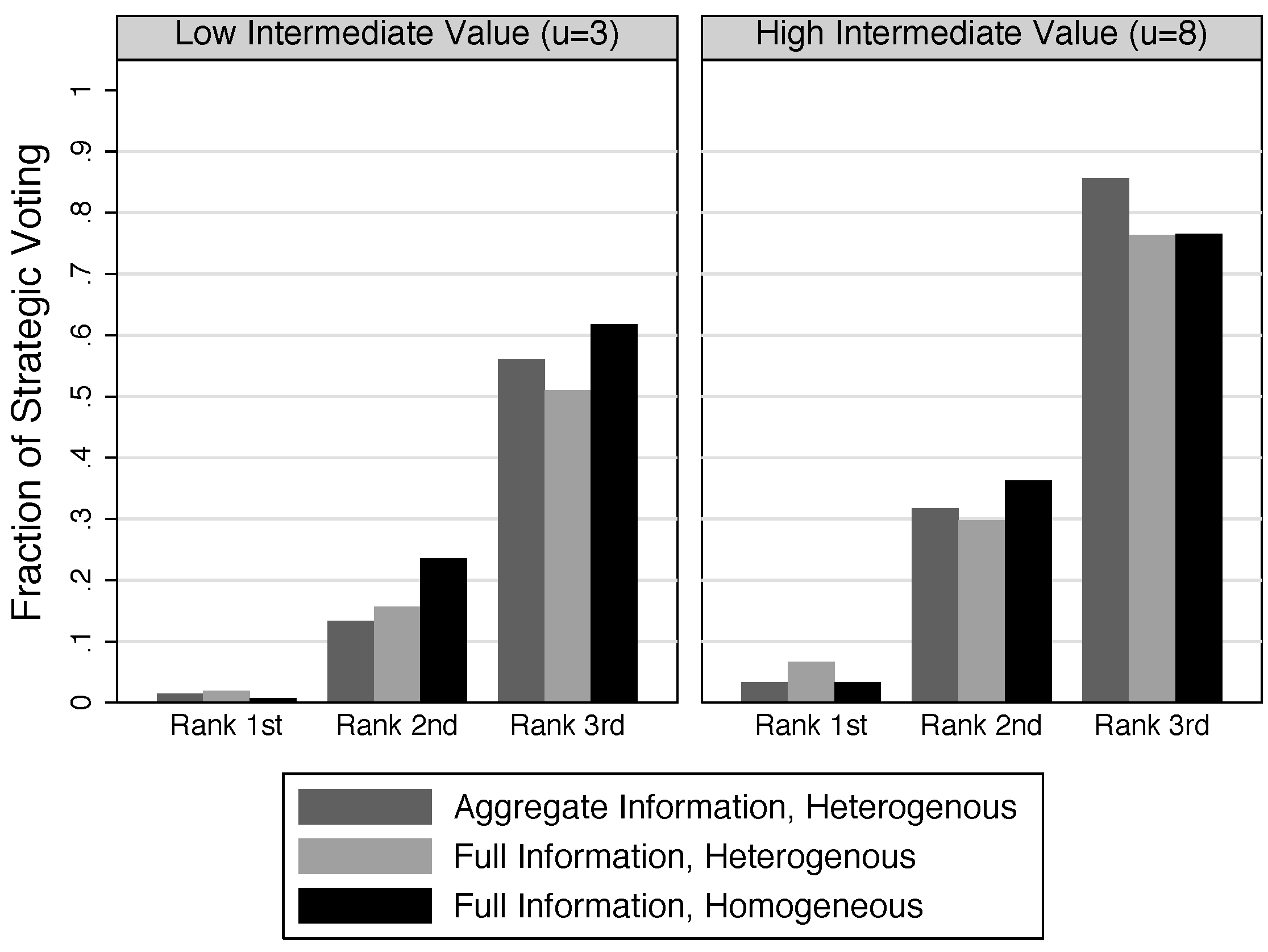
With information, Rank 3rd voters vote more strategically than other Rank-Types Figure 4).

(7)

Heterogeneity decreases the probability of strategic voting of Rank 3rd voters with high intermediate value (Figure 4).

(8)

Heterogeneity increases the probability of strategic voting of Rank 2nd voters with high intermediate value (Figure 4).

3. Experimental Design

The experimental design aims at studying the effect of preference heterogeneity on the decision to vote, when the relative importance of the intermediate option and the extent of information are varied. Appendix B provides a sample of the experimental instructions.

The electorate is fixed during a session and consists of 12 voters. A session consists of 40 elections, which are called “rounds”. The number of rounds is unknown to participants. There are 3 preference orderings, {(A, B, C); (B, C, A); (C, A, B)}, which are assigned with equal probability to each subject. There is a new draw of preferences before every election, independently across subjects and elections. In every election each subject is required to cast one vote for A, B or C. Plurality rule determines the winner, with ties broken by equal probability random draw. Subjects are paid in each round according to the rank of the winner in their own preference ordering. A subject is paid 10 points if the winner is ranked first and 1 point in case it is ranked last. To obtain preference heterogeneity, the value paid in case the winner is the intermediate option is also randomly drawn. Prior to the election, at the individual level and independently across subjects and elections, it takes either the value 3 or 8 with 50% probability each10. All this is common knowledge. Aggregate election results are shown to every subject after every election.

We vary information across treatments in a between-subject design. The three treatments vary in the amount of information voters have about each other’s preferences. In all treatments, subjects know the distributions from which preference orderings and value of the intermediate option are drawn. They also know at the start of an election their own ordering and value. In the uninformed treatment this is all that the subjects know when deciding whether or not to vote. With full information in each round, before casting their vote, subjects are informed about the realization of the aggregate preferences orderings and for each preference ordering, they are also told the realized distribution of intermediate preferences. Table 1 gives an example of the information provided.

Table 1. Example of Information Provided to Subjects.

Preference Ordering	Intermediate Value = 3	Intermediate Value = 8	Total
A B C	2	3	5
B C A	1	2	3
C A B	2	2	4

Notes. This table shows an example of the information provided to subjects in the full information treatment. Each row provides information about one of the possible preference orderings. Cells in columns 2 and 3 indicate the number of voters (including the subject concerned) in the electorate with value of the intermediate option of 3 or 8, respectively. Cells in the final column show the aggregate number for that row. In the aggregate information treatment, only the first and last columns were shown.

Table 1. Example of Information Provided to Subjects.

Preference Ordering	Intermediate Value = 3	Intermediate Value = 8	Total
A B C	2	3	5
B C A	1	2	3
C A B	2	2	4

Notes. This table shows an example of the information provided to subjects in the full information treatment. Each row provides information about one of the possible preference orderings. Cells in columns 2 and 3 indicate the number of voters (including the subject concerned) in the electorate with value of the intermediate option of 3 or 8, respectively. Cells in the final column show the aggregate number for that row. In the aggregate information treatment, only the first and last columns were shown.

The remaining treatment lies between uninformed and full disclosure of preferences. With aggregate information subjects know the aggregate preferences, but not the realized distribution of the intermediate values, i.e., they know only the prior distribution. This is done by providing only the first and last columns of Table 1, with subjects being aware that intermediate values may vary across voters.

Every experimental electorate experienced the same realizations of the random distribution of preference orderings, making it possible to directly compare across groups. This is the same realization as used for the homogeneous treatment in MT11 (c.f. Appendix C). The realization of the value for the intermediate option was also the same across groups.

The experiment was computerized using z-tree [27]. Ten sessions were run at the CREED laboratory at the University of Amsterdam in June 2009. 204 subjects11 participated, allowing for 17 independent electorates12. In addition to a show-up fee of €7, subjects were paid €0.05 per experimental point. Average earnings were €20.07, including the show-up fee. Each session lasted about one and a half hours.

4. Results

This results section will focus on analyzing the two main questions addressed in this paper: (i) what is the behavioral effect of heterogeneity on the level of strategic voting; (ii) which component of the information is more relevant for voting behavior: information on the aggregate preference ordering or information about the intensity of preferences. In the analysis to follow we first look at the comparative statics concerning the value of the intermediate option holding the remaining variables constant and then, holding fixed the intermediate value, we look at the effect of heterogeneity and/or information. Statistical tests are non-parametric, using average behavior of (sub-groups of) voters per electorate as the unit of observation. The grouping should be clear from the text. The statistical testing takes into account that sub-groups of voters within the same electorate are not independent.

4.1. Election Winner

A first question regards the election winner. More specifically we are interested in the probability that the candidate with the largest sincere support wins an election. As in TS11, we denote this candidate as the “Majoritarian Candidate”. Figure 5 shows the winning probability by the majoritarian candidate under each information setting13.

Notice that for the homogeneous treatments the addition of information increases the winning probability of the majoritarian candidate by 22 percentage points.14 To check for the effect of preference heterogeneity, we compare the homogeneous and heterogeneous uninformed treatments with their full information counterparts (first and last pairs of bars in Figure 5). It is clear from the graph that differences between the two treatments are small, both without information and with full information. Within each information treatment, the differences are indeed statistically indistinguishable for the uninformed sessions (Mann-Whitney (MW) rank-sum test, Z = 0.316, p = 0.751, N = 17) as well as for the (fully) informed sessions (MW, Z = ‒0.237, p = 0.813, N = 18).

Figure 5. Majoritarian Candidate Winning Probability.

Figure 5. Majoritarian Candidate Winning Probability.

Notes. Bars show for each treatment the fraction of elections won by the majoritarian candidate, counting as 0.5 (0.33) cases involving a two-way (three-way) tie, before the random tie breaking procedure. Appendix D provides the graph when excluding such ties. Note that information in the homogenous treatment is always full, because subjects (know that they) do not differ in value for the intermediate option.

To check the relative importance of the two kinds of information, we consider the aggregate information treatment. Note that in this treatment subjects have the same information about aggregate preferences as in full information, but no information regarding the intensity of preferences. From the graph it is clear that there is no substantial difference between the winning probability of the majoritarian candidate in the aggregate and full information treatments. Indeed, the difference turns out to be statistically insignificant (MW, Z = ‒1.137, p = 0.256, N = 12). This indicates that information about the aggregate distribution of preferences is sufficient to explain the probability increase in the full information treatment. Next, we will consider in more detail the voting patterns in distinct treatments.

4.2. Aggregate Behavior

We start by analyzing the uninformed treatments. Figure 6 shows the average fraction of strategic votes by period in the uninformed electorates, grouped by value of the intermediate option. A first look at the graphs suggest that there is more strategic voting when the intermediate value is high and that there is little difference between the homogeneous and heterogeneous treatments for given value of the intermediate option. These suggestions are confirmed by statistical tests, in line with behavioral predictions 1 and 2. Specifically, in line with prediction 1, strategic voting observed in voters with high intermediate value is statistically different from voters with low intermediate value both under heterogeneous preferences (Wilcoxon (W) signed-rank test, Z = ‒2.023, p = 0.043, N = 5) and under homogeneous preferences (MW, Z = ‒2.882, p = 0.004, N = 12). As for prediction 2, non-parametric tests cannot reject the hypothesis that heterogeneity has no effect on strategic voting when the intermediate value is high (MW, Z = ‒0.365, p = 0.715, N = 11), nor when it is low (MW, Z ≈ 0, p ≈ 1.000, N = 11).

Figure 6. Experimental Data and Predictions: Uninformed Treatment.

Figure 6. Experimental Data and Predictions: Uninformed Treatment.

Notes. Lines show the three-period moving average of the fraction of strategic votes in the uninformed heterogeneous (left panel) and uninformed homogeneous (right panel). The latter is taken from Figure 6a in MT11. Dashed (solid) lines refer to low (high) intermediate values. Horizontal lines show the MLE predictions (for µ = 0.55).

Also important to notice is that behavior is very much in line with the equilibrium predictions of the Quantal Response Equilibrium model. For these predictions, we use value µ = 0.55 for the noise parameter, which was obtained by ML estimation using data from a pilot session run for the homogenous treatment (see TS11 for more details). Figure 6 shows that observations for = 3 are close to the predicted level for both the homogeneous and heterogeneous cases. For = 8, there is slightly less strategic voting than predicted, but—as indicated above—the comparative static prediction of more strategic voting than for = 3 is supported in both cases.

Figure 7 shows similar graphs for the informed treatments. Again in line with behavioral prediction 1, voters with a high intermediate value are more likely to cast a strategic vote than voters with a low intermediate value (for the aggregate information, heterogeneous electorates: W, Z = −2.201, p = 0.028, N = 6; for the full information, heterogeneous electorates: W, Z = −2.201, p = 0.028, N = 6; for the full information, homogeneous electorates: MW, Z = −2.882, p = 0.004, N = 12).

When checking for the effect of heterogeneity on average behavior, behavioral prediction 3 finds partial support. It predicts no effect of heterogeneity. For the voters with high intermediate option, there is indeed no statistically significant effect (Kruskal-Wallis (KW) test, χ² = 0.327, p = 0.849, N = 18), whereas for the voters with low intermediate value there is (KW, χ² = 9.564, p = 0.008, N = 18). This difference is due to the higher rate of strategic voting by homogeneous voters (16.87%) compared to heterogeneous voters (12.62%). In contrast to the case without information, when information is provided, heterogeneity does reduce the extent of strategic voting for voters who attribute a relatively low value to the intermediate option.

Figure 7. Experimental Data and Predictions: Informed Treatments.

Figure 7. Experimental Data and Predictions: Informed Treatments.

Notes. Lines show the 3-period moving average of the fraction of strategic votes. The top left (right) panel shows the aggregate (full) information case with heterogeneous preferences and the lower panel show the homogenous case. “Low” and “High” refer to the value of the intermediate option. Note that the MLE prediction in a round depends on the realized distribution of preferences, the realized intensity of preferences and voter’s information. Results for the homogenous case are taken from TS11.

Recall that information may concern the realized distribution of preference orderings alone, or in combination with the realizations on intermediate valuations. We consider which type of information affects strategic behavior most strongly. Our evidence indicates that the value realizations add little to the effect of aggregate information about preferences. This is in line with behavioral prediction 4. It can be seen from the lack of statistical difference when comparing the two heterogeneous informed treatments in Figure 7. For low intermediate values: MW, Z = −0.080, p = 0.936, N = 12; for high intermediate values: MW, Z = 0.0160, p = 0.873, N = 12). In other words, heterogeneity of preferences diminishes strategic voting (when the intermediate value is low), but detailed information about the intensity of preferences does not add to this effect.

Finally, behavioral prediction 5 concerns the comparative static of strategic behavior in the uninformed treatments versus the informed treatments. As predicted for the heterogeneous treatments, this average is higher with information (compare the first two panels of Figure 7 to the first panel in Figure 6). The differences are statistically significant (for low intermediate values: MW, Z = −2.485, p = 0.013, N = 17; for high intermediate values: MW, Z = −1.899, p = 0.058, N = 17). In TS11, we observed a similar effect of information for the homogenous case.

4.3. Strategic Voting by Rank-Type

Next, we focus specifically on the informed treatments. As outlined above, in these treatments we can group subjects according to their Rank-Type. Figure 8 shows the average fraction of strategic voting for each Rank-Type, grouped by the value of the intermediate option. For each Rank-Type, the figure separately shows strategic voting under each informed treatment.

First note that—as expected—Rank 1st voters rarely vote strategically. For each intermediate value, Rank 3rd voters are most likely to vote strategically. The differences are significant when comparing to both Rank 2nd and Rank 1st voters, both for low intermediate values and for high intermediate values (W, Z = −2.201, p = 0.0277, N = 6; for all pairwise comparisons). This is in line with an intuition from Duverger’s Law and behavioral prediction 6. The comparative statics within Rank-Types of intermediate value are as expected, since the fraction of strategic voting is statistically higher when the importance of the intermediate option is high, for each and every group (p < 0.05 for all comparisons, using W or MW test where appropriate, N = 6).

Figure 8. Level of Strategic Voting by Rank-Type

Figure 8. Level of Strategic Voting by Rank-Type

Notes. Bars show the fraction of vote that was strategic, grouped by the value of the intermediate option. Voter Rank-Types are distinguished along the horizontal axis and treatments by the color of the bar. Results for the homogenous case are taken from TS11.

When checking for the effect of heterogeneity, our results do not provide support for behavioral predictions 7 and 8. It was predicted from the QRE analysis that for voters with high intermediate value, heterogeneity would increase the likelihood of a strategic vote for Rank 2nd voters and reduce it for Rank 3rd voters (behavioral predictions 7 and 8). The general result is, if any, a reduction in the strategic voting probability for Rank 2nd voters15 and no reduction for Rank 3rd voters16. Moreover, with the exception of Rank 3rd voters with high intermediate value, all comparative statics indicate a lower probability under heterogeneity when compared to homogeneity. This seems to indicate that when the complexity of the situation increases, subjects tend to move to simpler heuristics, such as sincere voting. We will return to this point, below.

When investigating which element of the information provided is determinant of strategic behavior, the evidence is once more in favor of the aggregate information. For the comparison of aggregate to full information we cannot reject the null hypothesis of these coming from the same distribution on any sub-group (W, N = 12, all p > 0.46), with the exception of the sub-group of heterogeneous Rank 3rd voters with high intermediate values (W, Z = 2.262, p = 0.024, N = 6). Therefore, the additional information on the intensity seems to have little effect on strategic voting behavior, even when considering voters in subgroups, based on their rank.

All in all, heterogeneity seems to reduce the overall level of strategic voting. However, the differences across Rank-Types and the differences between low and high intermediate options are much more pronounced than the effect of heterogeneity. These results provide further support to two claims. First, the main comparative statics reported in in TS11 on the effects of information and intermediate value on strategic voting are robust with respect to preference heterogeneity. Second, information about aggregate orderings is driving these results.

5. Concluding Remarks

In this paper we have studied the effect of preference heterogeneity in strategic voting and its interaction with information. We also investigated which element of the information provided to voters is more relevant to understand and predict behavior. We built on the model introduced in our companion paper TS11. In that model, only the preference ordering distinguishes between voters; the intensity of the preferences is kept homogeneous. We introduce here heterogeneity by allowing the intensity of preferences to vary within an electorate (and across rounds). This also allows us to decompose the information provided to voters into two pieces: information about the aggregate preferences and information concerning the intensity of those preferences.

Our experimental data support most of the behavioral predictions derived from the model. In particular, we observe (i) that strategic voting increases as the value of a voter’s second best option increases and (ii) more strategic voting occurs with information than without. Also, (iii) Rank-3rd voters are more likely to vote strategically than other voters. Partial support is obtained concerning the effect of heterogeneity. We observe no effect of heterogeneity for uninformed voters (as predicted) but a negative effect on informed voters, when the prediction was also neutral. Hence, (iv) heterogeneity decreases strategic voting when voters are informed about the distribution of preferences. Moreover, (v) both Rank-2nd (against prediction) and Rank-3rd (as predicted) voters are negatively affected by heterogeneity. Finally, data support the behavioral prediction that (vi) information about the aggregate preferences is determinant for behavior. We observe that the additional information about intensity of preferences add very little to behavior both in the theoretical analyses and in the experimental data.

We conclude that the overall effect of heterogeneity is a reduction in the probability of a strategic vote. This is in line with general argumentations about bounded rationality, which point to a choice of simpler heuristics, such as sincere voting, once the complexity of the environment increases. It seems reasonable to assume that compared to the homogenous case, heterogeneity makes the environment much more complex for a voter to oversee. Now, she not only needs to take into account that other voters may think differently about what are the best (and second-best) alternatives, she also has to contemplate that some voters care more about their second best than others. It is quite intuitive that this would lead more voters to choose the “simpler” option of voting for the alternative they like best. In terms of effect size, however, heterogeneity comes second to both the value of a voter’s second best option as to her Rank-Type. This indicates that the general comparative static results reported in TS11 are stable even in this more complex environment.

Before one can derive possible policy implications from our results, future analysis is needed that test their robustness to increased electorate size and different subject pools. For this purpose, one can think of field experiments with online elections, for example. We consider such field experiments as a natural next step on the way to better understanding strategic voting and the effects of preference heterogeneity.

References

- Bosman, R.; Hennig-Schmidt, H.; van Winden, F. Exploring group decision making in a power-to-take experiment. Exp. Econ. 2006, 9, 35–51. [Google Scholar] [CrossRef]
- Forsythe, R.; Myerson, R.; Rietz, T.; Weber, R. An experiment on coordination in multi-candidate elections: The importance of polls and election histories. Soc. Choice Welf. 1993, 10, 223–247. [Google Scholar]
- Forsythe, R.; Rietz, T.; Myerson, R.; Weber, R. An experimental study of voting rules and polls in three-candidate elections. Int. J. Game Theory 1996, 25, 355–383. [Google Scholar] [CrossRef]
- Morton, R.; Williams, K. Information asymmetries and simultaneous versus sequential Voting. Am. Polit. Sci. Rev. 1999, 93, 51–67. [Google Scholar] [CrossRef]
- Myerson, R.; Weber, R. A theory of voting equilibria. Am. Polit. Sci. Rev. 1993, 87, 102–114. [Google Scholar] [CrossRef]
- Tyszler, M. Political Economics in the Laboratory. Ph.D. Thesis, University of Amsterdam, Amsterdam, The Netherlands, 2012. [Google Scholar]
- Tyszler, M.; Schram, A. Information and Strategic Voting; Tinbergen Institute Discussion Papers TI 2011, 025/1; Tinbergen Institute: Amsterdam, The Netherlands, 2011. [Google Scholar]
- Erlei, M. Heterogeneous social preferences. J. Econ. Behav. Organ. 2008, 65, 436–457. [Google Scholar] [CrossRef]
- Fischbacher, U.; Gaechter, S. Heterogeneous Social Preferences and the Dynamics of Free Riding in Public Goods; Discussion Paper No. 2011; IZA: Bonn, Germany, 2006. [Google Scholar]
- Andersen, S.; Harrison, G.; Lau, M.; Rutström, E. Preference heterogeneity in experiments: Comparing the field and laboratory. J. Econ. Behav. Organ. 2010, 73, 209–224. [Google Scholar] [CrossRef]
- Duch, R.; Stevenson, R. Context and economic expectations: When do voters get it right? Br. J. Polit. Sci. 2011, 41, 1–31. [Google Scholar] [CrossRef]
- Rivers, D. Heterogeneity in models of electoral choice. Am. J. Polit. Sci. 1988, 32, 737–757. [Google Scholar] [CrossRef]
- Conlisk, J. Why bounded rationality? J. Econ. Lit. 1996, 34, 669–700. [Google Scholar]
- Schwenk, C. Cognitive simplification processes in strategic decision-making. Strateg. Manag. J. 1982, 5, 111–128. [Google Scholar] [CrossRef]
- McKelvey, R.; Palfrey, T. Quantal response equilibria for normal form games. Games Econ. Behav. 1995, 10, 6–38. [Google Scholar] [CrossRef]
- Goeree, J.; Holt, C. An explanation of anomalous behavior in models of political participation. Am. Pol. Sci. Rev. 2005, 99, 201–213. [Google Scholar]
- Groβer, J.; Schram, A. Public opinion polls, voter turnout, and welfare: An experimental study. Am. J. Polit. Sci. 2010, 54, 700–717. [Google Scholar] [CrossRef]
- Levine, D.; Palfrey, T. The paradox of voter participation? A laboratory study. Am. Polit. Sci. Rev. 2007, 101, 143–158. [Google Scholar] [CrossRef]
- Blais, A.; Nadeau, R. Measuring strategic voting: A two-step procedure. Elect. Stud. 1996, 15, 39–52. [Google Scholar] [CrossRef]
- Blais, A.; Nadeau, R.; Gidengil, E.; Nevitte, N. Measuring strategic voting in multiparty plurality elections. Elect. Stud. 2001, 20, 343–352. [Google Scholar] [CrossRef]
- Cain, B.E. Strategic voting in Britain. Am. J. Polit. Sci. 1978, 22, 639–655. [Google Scholar] [CrossRef]
- Höchtl, W.; Sausgruber, R.; Tyran, J.-R. Inequality aversion and voting on redistribution. Eur. Econ. Rev. 2012, 56, 1406–1421. [Google Scholar] [CrossRef]
- Messer, K.; Poe, G.; Rondeau, D.; Schulze, W.; Vossler, C. Exploring voting anomalies using a demand revealing random price voting mechanism. J. Pub. Econ. 2010, 94, 308–317. [Google Scholar] [CrossRef]
- Fey, M. Stability and coordination in Duverger’s Law: A formal model of preelection polls and strategic voting. Am. Polit. Sci. Rev. 1997, 91, 135–147. [Google Scholar] [CrossRef]
- Palfrey, T. A Mathematical Proof of Duverger’s Law. In Models of Strategic Choice in Politics; Ordershook, P., Ed.; The University of Michigan Press: Ann Arbor, MI, USA, 1989; pp. 69–91. [Google Scholar]
- Riker, W. The two-party system and Duverger’s law: An essay on the history of political science. Am. Polit. Sci. Rev. 1982, 76, 753–766. [Google Scholar] [CrossRef]
- Fischbacher, U. z-Tree: Zurich toolbox for ready-made economic experiments. Exp. Econ. 2007, 10, 171–178. [Google Scholar] [CrossRef]
Appendix A. A Selection of Nash Equilibria
Uninformed
Aggregate Information
Full Information