Noncontractible Investments and Reference Points

Abstract

We analyze noncontractible investments in a model with shading. A seller can make an investment that affects a buyer’s value. The parties have outside options that depend on asset ownership. When shading is not possible and there is no contract renegotiation, an optimum can be achieved by giving the seller the right to make a take-it-or-leave-it offer. However, with shading, such a contract creates deadweight losses. We show that an optimal contract will limit the seller’s offers, and possibly create ex post inefficiency. Asset ownership can improve matters even if revelation mechanisms are allowed.

1. Introduction

In the last twenty five years or so a formal literature on asset ownership and firm boundaries—known as property rights theory—has developed. This theory is based on the idea that parties write incomplete contracts ex ante and that the allocation of asset ownership influences how contracts are completed ex post. In the standard model, parties reach an ex post efficient outcome through renegotiation once the state of the world is realized. However, the ability to exercise residual control rights increases the incentive of an asset owner to make noncontractible relationship-specific investments, and, as a consequence, it is optimal to assign asset ownership to those whose investments are most important¹. Empirical support for the idea that noncontractible investments are influenced by asset ownership can be found in a number of papers, including Woodruff [5], Baker and Hubbard [6,7], Acemoglu et al. [8], and Gebhardt [9]; see also the discussion of franchising in Lafontaine and Slade [10].

As is now well known, one weakness of the property rights theory is that in the standard model only a particular class of contracts is considered. Specifically, revelation mechanisms of the Moore-Repullo-Maskin-Tirole type (in combination with third parties and/or lotteries) can do better and indeed often achieve the first-best. Such mechanisms are not observed in reality but they pose a challenge to the theory.

Partly to overcome this weakness, an alternative approach has recently been developed based on the idea that contracts are reference points². According to this approach a contract, negotiated under (relatively) competitive conditions, circumscribes or delineates parties’ feelings of entitlement. Parties do not feel entitled to outcomes outside the contract, but, possibly as a result of self-serving biases, may feel entitled to different outcomes within the contract. In the simplest version each party feels entitled to the best outcome within the contract³. When a party does not receive his entitlement, he feels aggrieved and retaliates by shading in noncontractible ways, hurting the other party, and creating deadweight losses⁴. Under these assumptions, a more open-ended contract leads to more aggrievement and shading, and there is an optimal degree of contractual flexibility. Revelation mechanisms do not achieve the first-best because they depend on the existence of many possible outcomes, and therefore cause shading. In Hart [16], and Hart and Holmstrom [17], this approach is used to develop theories of asset ownership and firm boundaries.

So far, the literature on contracts as reference points has focused on ex post inefficiency and has downplayed noncontractible investments. An open question is whether the newer approach can incorporate such investments and whether it is consistent with the empirical findings, referred to above, that asset ownership influences such investments. The purpose of the present paper is to provide a positive answer to this question.

We develop a simple model in which a seller invests in the quality of a good or service provided to a buyer (thus the investment is a “cross-investment” in the sense of MacLeod and Malcomson [18] or Che and Hausch [19]). The investment is discrete (invest or don’t invest), while ex post trade is continuous and can be any level between zero and one. The buyer’s value can be high or low, and the seller’s investment affects the probability that the value is high. Value is observable to both parties but not verifiable. The buyer and seller have outside options that depend on the ex ante allocation of asset ownership and the value of the good. There are always gains from trade and so in an ideal world trade would always take place at the level one.

In our model, in contrast to much of the literature on contracts as reference points, specific performance is allowed. Therefore, in the absence of investment the first-best could easily be achieved with a contract that mandates trade at level one at a fixed price. Specific performance generates no shading since the contract is rigid and contains only one outcome. In such a setting, asset ownership would have no role.

However, a specific performance contract does not achieve the first-best in the presence of investment. The seller has no incentive to invest since she receives the same price whether value is high or low. In order to encourage investment the parties will choose a more flexible contract; for example, they might allow the seller to make a take-it-or-leave-it offer to the buyer. In this paper we will rule out renegotiation and so in the absence of shading such a contract would achieve the first-best: the seller receives all the surplus and so has the socially correct investment incentives. However, in the presence of shading such a contract does not achieve the first-best since the buyer will feel aggrieved when the seller chooses a high price. We will show that the first-best is generally no longer attainable, and that the parties face a trade-off between providing investment incentives, achieving ex post efficiency, and avoiding shading.

We find that there are two leading candidates for an optimal contract if investment is desired. In one, ex post efficient trade is achieved but the parties restrict the range of prices from which the seller can choose ex post to be as small as possible subject to the seller having an incentive to invest. This contract will lead to some shading. The second contract introduces some ex post inefficiency by allowing the seller to choose between two ex post outcomes: trade at a level of one at a high price or trade at a level below one at a low price (equivalently trade with probability less than one). The outcomes are designed so that the buyer is indifferent between the two outcomes if value is high, but strictly prefers the low trade outcome if value is low. In this contract, there is no shading. In Section 2, we show that, in the absence of asset ownership and outside options, one of the above two contracts, or specific performance (which yields no investment), is second-best optimal.

In Section 3, we introduce asset ownership and show that this can improve matters. First, suppose that the optimal contract is one that creates ex post inefficiency. Then an allocation of asset ownership that yields a high outside option for the seller in the low value state raises total surplus by increasing efficiency when trade does not take place. Second, suppose that the optimal contract is one that allows the seller to choose from a range of prices. Then an allocation of asset ownership that yields a high outside option for the seller in the high value state will reduce the buyer’s feelings of aggrievement, and hence shading, to the extent that the buyer does not feel entitled to an outcome where the seller’s payoff is below her outside option.

The effect of allocating assets to the buyer is more ambiguous. As with the seller, a high outside option for the buyer in the low value state increases surplus by providing higher value when trade does not take place. However, a high outside option for the buyer in the high value state reduces the amount that the seller can charge in this state, lowering the seller’s incentive to invest.

In Section 4, we show that our results are robust to the introduction of revelation mechanisms. In particular, for the case where the seller’s outside options are independent of her investment, the contracts analyzed in Section 2 and Section 3 continue to be optimal⁵.

As noted, in this paper we rule out renegotiation. We do this mainly because revelation mechanisms are most powerful if parties can commit not to renegotiate and we want to show that even under these conditions asset ownership matters. However, the absence of renegotiation can also be justified on the grounds that (opportunistic) renegotiation can lead to (even) higher levels of aggrievement and shading and so parties may be discouraged from attempting it (see Hart and Moore [11] and Hart [16] for discussions, and Fehr et al. [21] for experimental evidence). We discuss briefly how renegotiation would affect our results in Section 5. We also consider some other extensions in this section.

The paper is organized as follows. The model is presented in Section 2 for the special case where outside options are zero. Asset ownership and outside options are introduced in Section 3. Section 2 and Section 3 focus on a particular class of contracts. In Section 4, general revelation game contracts are considered and the contracts of Section 2 and Section 3 are shown to be optimal under certain conditions. Section 5 concludes.

2. The Model

We consider a buyer and seller who can trade a good. There are three dates. At date 0 the parties meet and contract. At date ½, the seller can make a noncontractible investment that affects the quality of the good. At date 1 trade occurs.

For the moment, we suppose that the parties’ outside options are zero; we relax this assumption in Section 3 and Section 4. We assume that there are two states of the world, high and low. The value of the good is v_H in the high state and v_L in the low state, where v_H > v_L > 0. The seller can affect the probability of the high state through her investment. If the seller invests, the probability that the state is high is π, where 0 < π < 1. For simplicity, we suppose that, if the seller does not invest, the state is low with probability 1. The seller incurs a nonverifiable cost c > 0 if she invests. Both parties learn the value of v just before date 1 (and hence before they trade); however, v is not verifiable. The seller’s variable costs at date 1 are zero. There is no discounting and both parties are risk neutral and have no wealth constraints.

In the first-best trade would always occur at date 1 since v_L > 0; and investment would take place as long as the social gain exceeds the social cost:

π v_H + (1 − π) v_L − c > v_L

(1)

that is,

π (v_H − v_L) > c

(2)

We will be interested in the case where (2) holds. In contrast to the previous literature on contracts as reference points, we suppose that, if trade fails to occur, it is clear who is responsible and so that party can be penalized. Thus, if (2) does not hold, it is easy to achieve the first-best with a specific performance contract: trade is mandated at date 1 at a fixed price; a party who refuses to trade has to pay large damages. However, if (2) holds, a specific performance contract does not achieve the first-best since the seller has no incentive to invest: she receives the same price whether v is high or low. (Of course, if v were verifiable, price could be made contingent on v.)

In the second-best, a contract will consist of a set of trade-price vectors and a mechanism for choosing among them at date 1. This mechanism will be played after v is realized. We will assume that partial trade is feasible; this is never optimal in the first-best. Denote a typical trade-price vector by (λ, p), where 0 ≤ λ ≤ 1 is the quantity traded and p is the price. That is, the buyer pays the total amount p for receiving the quantity of the good λ. The buyer’s payoff is λv − p, and the seller’s payoff is p (ignoring investment costs). Note that an alternative interpretation is that with probability λ the buyer and seller trade, and with probability 1 − λ they do not, but either way the buyer always pays the seller p.

We follow Hart and Moore [11] in supposing that there is a competitive market for buyers and sellers at date 0 and so both parties feel that the initial contract is “fair”. Thus the initial contract is a reference point for entitlements. At date 1 the buyer and seller are in a situation of bilateral monopoly. At this point, the parties may feel entitled to different outcomes within the contract. As in Hart and Moore [11] we suppose that each party feels entitled to the best outcome, and if he does not get it he will be aggrieved and will shade, creating deadweight losses. In this and the next section, but not in Section 4, we will restrict attention to voluntary trade contracts in which each party can quit ex post without penalty. In this case, we compute aggrievement and shading as follows. A party’s entitlement is given by his maximized payoff over all possible contractual outcomes, subject to the other party’s (ex post) participation constraint being satisfied; that is, the other party does not quit. Aggrievement is the difference between the party’s entitlement and the payoff the party actually receives. A party who is aggrieved shades (shading is not contractible). Shading equals aggrievement multiplied by θ, where 0 < θ < 1. Shading reduces the other party’s payoff by the amount of shading without affecting the payoff of the shading party⁶.

Let’s start with the case where there is no shading: θ = 0. Since in this paper we rule out renegotiation (but see the discussion in the conclusions), it is then easy to achieve the first-best. The parties can simply agree in advance that the seller will make a take-it-or-leave-it offer to the buyer at date 1. The seller will propose price p = v_H in the good (high value) state, price p = v_L in the bad (low value) state, the buyer will accept and the seller will capture the entire surplus. This gives the seller the socially correct investment incentives. (Lump sum transfers can be used to divide up the surplus ex ante.)

If θ > 0, however, a contract that allows the seller to pick p_H = v_H or p_L = v_L does not achieve the first-best. In the good state the seller will propose v_H, and the buyer will accept this, but he will feel entitled to the lower price v_L (the best outcome for him consistent with the contract), and will shade by θ (v_H − v_L). The buyer will not shade in the bad state since he receives the lowest possible contractual price, and the seller will not shade in the good state since she receives the highest possible contractual price. Finally, the seller will not shade in the bad state since she does not feel entitled to an outcome in which the buyer makes a loss (i.e., quits)⁷.

One way the parties can reduce shading is to restrict the range of allowable prices. Suppose that they agree that the seller can choose either p_H, where v_H ≥ p_H > v_L, or p_L = v_L. Then the buyer’s shading in the good state is reduced to θ (p_H − v_L). The seller’s payoff in this state net of shading costs is p_H−θ (p_H − v_L) ≥ 0. The condition for the seller to invest is thus:

π (p_H − θ (p_H − v_L)) + (1 − π) v_L − c ≥ v_L

(3)

that is,

π (p_H − v_L)(1 − θ) ≥ c

(4)

Shading is minimized if (4) holds with equality, and so we can solve for p_H. We need to check that the buyer is willing to pay p_H in the good state:

v_H ≥ p_H

(5)

that is,

(6)

((6) will not hold if θ is close to 1.) Gross social surplus (ignoring the investment cost c) is given by

(7)

For future reference we call this contract, where λ_H = λ_L = 1, p_H = + v_L, p_L = v_L, the “efficient trade” contract, since λ = 1 in both states.

Another way for the parties to reduce shading is to make the (λ, p) outcome in the bad state less attractive to the high value buyer. As in the asymmetric information literature, this can be achieved by reducing λ_L. Let (λ_H, p_H), (λ_L, p_L) denote the trade-price vectors in the good and bad states respectively. Keep λ_H = 1 and choose λ_L so that the high value buyer is indifferent between (λ_H, p_H) and (λ_L, p_L). This yields

v_H − p_H = λ_Lv_H − p_L

(8)

Since the high value buyer is indifferent, he is not aggrieved and does not shade. Thus the condition for the seller to invest is now

π (p_H − p_L) ≥ c

(9)

Combining (8) – (9) yields

(10)

For ex post efficiency reasons we want λ_L to be as large as possible and so (10) will hold with equality. We continue to set p_L = _Lv_L, so that the buyer breaks even in the bad state. This ensures that the seller chooses (λ_L, p_L) in the bad state and that there is no seller aggrievement: the seller does not feel entitled to an outcome where the buyer would quit. The gross surplus from this contract is

(11)

For future reference we call this contract, where λ_H = 1, λ_L = 1 – , p_H = + λ_Lv_L, p_L = λ_Lv_L, the “no aggrievement” contract.

The general analysis in Section 4 allows us to establish that either specific performance (yielding no investment) or one of the above two contracts—“efficient trade” or “no aggrievement”—is optimal.

Proposition 1.

(1)

If max (v_L, S₁ − c, S₂ − c) = v_L the optimal contract is specific performance. Net surplus is v_L.

(2)

If max (v_L, S₁ − c, S₂ − c) > v_L then there is an optimal contract of the following form: the seller chooses between (λ_H, p_H) and (λ_L, p_L) at date 1 and the buyer can reject without penalty (leading to no trade), where

(2a)

If max (v_L, S₁ − c, S₂ – c) = S₁ − c, λ_H = λ_L = 1, p_H = + v_L, p_L = v_L (the “efficient trade” contract). Net surplus is S₁ − c.

(2b)

If max (v_L, S₁ − c, S₂ − c) = S₂ − c, λ_H = 1, λ_L = 1 – , p_H = + λ_L v_L, p_L = λ_Lv_L (the “no aggrievement” contract). Net surplus is S₂ − c.

Note that in Case 2a, S₁ − c > v_L, and it is easy to show that this implies (6)⁸.

It follows immediately from Proposition 1 that, if investment is first-best efficient ((2) holds), then the second-best is strictly inferior to the first-best: in (1) there is no investment, and in (2) there is shading or inefficient trade. At the same time note that, if θ is close to zero, the “efficient trade” contract approximates the first-best, since there is very little shading; and, if v_L is close to zero, the “no aggrievement” contract approximates the first-best, since the efficiency losses from inefficient trade in the bad state are small.

3. Asset Ownership and Outside Options

We have seen in Section 2 that if (2) holds the first-best cannot be achieved. It is thus natural to ask how the second-best outcome might be improved. The property rights literature suggests that asset ownership helps. We explore this here.

We take the view that asset ownership affects outside options. In particular, an allocation of asset ownership at date 0 permits the seller to achieve in the high value and low value state, respectively, without trading with the buyer; and the buyer to achieve in the high value and low value state without trading with the seller. Note that the buyer’s outside option may vary with the seller’s investment to the extent that the seller’s noncontractible investment in quality can be appropriated by the buyer, e.g., it is embodied in a physical asset rather than in the seller’s human capital or represents an idea that the buyer can “steal”.

We suppose that the parties’ payoffs are linear in the level of trade. Thus, under the trade-price vector (λ, p) in state j (j = H, L) the buyer’s payoff is equal to λ times his payoff under the contract (1, p) plus (1 − λ ) times his payoff under the contract (0, p); that is, the buyer’s payoff is

(12)

An equivalent interpretation is that with probability λ the buyer trades with the seller and with probability 1 − λ the buyer trades on the outside market, but either way the buyer always pays the seller p.

Similarly, the seller’s payoff is

(13)

We assume

(14)

and that ex post trade is always efficient:

(15)

We also suppose

(16)

and

(17)

(16) says that the net surplus from the relationship is higher in the good state than in the bad one. In other words, the investment enhances the value of the relationship. (17) ensures that the seller will want to invest in the case of no shading when she can make a take-it-or-leave-it offer to the buyer⁹. Note that if the seller’s investment is purely an investment in the seller’s human capital, then = , and (17) is implied by (2). (16) and (17) both limit how much can exceed ¹⁰.

As in Section 2, if no investment is desirable, the first-best can be achieved with a specific performance contract. From now on, we focus on the investment case. It is helpful to divide our analysis into two subcases. We start with the situation where the seller’s outside option does not vary with her investment, e.g., because the seller’s investment is specific to the buyer:

(18)

(18) is restrictive, but it turns out that this case is tractable and instructive.

It is useful to compute the analogous contracts to the “efficient trade” and “no aggrievement” contracts in Section 2. The “efficient trade” contract is characterized by

(19)

In (19), the buyer’s participation constraint is binding in the bad state. The buyer is aggrieved by in the good state since the seller earns above her outside option when receiving p_L ((15) and (18) imply that ); hence, the buyer feels entitled to pay p_L. The seller is indifferent between investing and not (see (3) with v_L replaced by p_L). The condition that the buyer does not quit in the good state is

(20)

Surplus from this contract is given by S₁,as in (7).

We see that the seller’s outside options have no effect on the surplus in the efficient trade contract given that

Turn next to the “no aggrievement” contract. The condition that the high value buyer is indifferent between the high and low value outcomes, which implies that he does not shade, becomes

(21)

and the condition for the seller to be just willing to invest is

(22)

Finally, the condition that the buyer’s participation constraint is binding in the bad state is

(23)

that is,

(24)

Combining (21) – (22) yields

(25)

To sum up, the “no aggrievement” contract is: λ_H = 1,λ_L = 1 − , p_H = + + λ_L , p_L = λ_L(v_L − ). Surplus under the “no aggrievement” contract is

(26)

As shown in Section 4, under (18), Proposition 1 generalizes as long as a further condition, (27), holds:

(27)

It is easy to check that the first inequality in (27) holds if and only if the “efficient trade” contract (see (19)) generates strictly higher surplus than specific performance. Thus (27) guarantees that, whenever “efficient trade” is strictly superior to specific performance, (20) holds. Note that (27) is automatically satisfied if is close to (and certainly if = ).

Proposition 2.

Assume = and (27). Then:

(1)

If max (v_L, S₁ − c, − c) = v_L the optimal contract is specific performance. Net surplus is v_L.

(2)

If max (v_L, S₁ − c, − c) > v_L, then there is an optimal contract of the following form: the seller chooses between (λ_H, p_H) and (λ_L, p_L) at date 1 and the buyer can reject without penalty (leading to no trade), where

(2a)

If max (v_L, S₁ − c, − c) = S₁ − c, λ_H = λ_L = 1, p_H = + v_L − , p_L = v_L − (the “efficient trade” contract). Net surplus is S₁ − c.

(2b)

If max (v_L, S₁ − c, − c) = − c, λ_H = 1, λ_L = 1 − , p_H = + + λ_L(v_L − − ), p_L = λ_L (v_L − )( the “no aggrievement” contract). Net surplus is − c.

If we compare S₂ with we see that the presence of an outside option for the seller strictly increases surplus in the “no aggrievement” contract: = S₂ when = = = 0 and is strictly increasing in . However, the effect of an outside option for the buyer is ambiguous. strictly increases if goes up, or if , go up equally, but it strictly decreases if goes up. The intuition behind these results is as follows. An increase in has two effects. It decreases the seller’s incentive to invest and hence λ_L in (25) must fall to compensate for this; but it also decreases the effects of inefficient trade since value outside the relationship is higher. The second effect dominates. An increase in has only the second effect and so increases surplus. An increase in unambiguously decreases surplus because it reduces the amount the seller can be paid in the good state and hence λ_L in (25) must fall to restore the seller’s investment incentives; and the increase in has no beneficial effect on ex post efficiency since λ_H = 1, i.e., is never earned.

In sum, seller outside options are unambiguously good for surplus (given (18)), whereas buyer options need not be (since they may discourage seller investment). However, buyer outside options are good for surplus if =

We now turn to the case where > . This case is in many ways more interesting since the property rights literature suggests that a higher outside option in the good state will encourage the seller to invest. Unfortunately, the case is also more complex, the results of Section 4 do not apply, and I have been unable to solve for an optimal contract. Thus, we will simply characterize some leading contracts.

Consider the contracts in Proposition 2. Make one small change in the assumption about aggrievement. Suppose that if p_H, p_L are the contractual prices then the parties feel entitled to any price in the range (p_L, p_H), not just to p_L, p_H¹¹. Start with the “efficient trade” contract in (19). In the presence of outside options the buyer does not expect to pay less than in the good state and so if > v_L − , his aggrievement and shading in the good state will be lower than before (previously the buyer felt entitled to pay v_L – ). In fact, if π ( + – v_L) ≥ c, we can achieve the first-best: set p_L = v_L − , p_H = . The buyer is not aggrieved in the good state because he does not feel entitled to an outcome where the seller would quit; and the buyer does not quit himself since, by (15), v_H − > . The buyer is not aggrieved in the bad state since he pays the lowest price. The seller is not aggrieved in the good state since she receives the highest price, and she is not aggrieved in the bad state since the buyer’s participation constraint is binding. Finally, the seller has an incentive to invest since π ( + – v_L) ≥ c.

Next assume that > v_L − but that π ( + − v_L) < c.Now the first-best cannot be achieved. The constraint that the seller is just willing to invest becomes

(28)

that is, if we set p_L = v_L − , so that the buyer’s participation constraint is binding in the bad state,

(29)

Given the shading in the good state equal to θ (p_H − ), social surplus is

(30)

The third case is where > v_L – . Here the analysis is as in Section 2. Combining the above three cases, we can write the general formula for the gross social surplus from the “efficient trade” contract as

(31)

The “no aggrievement” contract in Proposition 2 is unchanged. However, if > v_L − and , there is now a second “no aggrievement” contract. To see why, suppose that we set λ_H = 1 and p_H = . Then because the buyer does not expect the seller to earn less than her outside option the buyer will not be aggrieved in the good state even if he strictly prefers (λ_L, p_L) to (λ_H, p_H). Now choose (λ_L, p_L) so that the buyer’s participation constraint is binding in the bad state and the seller has an incentive to invest:

(32)

(33)

(32)–(33) yield

(34)

Note the role of the condition : without this, λ_L would be negative. For ex post efficiency reasons we want λ_L to be as large as possible, but λ_L cannot exceed 1. Thus maximal gross surplus from this second “no aggrievement” contract is

(35)

To emphasize again: this contract produces no aggrievement or shading since in the good state the buyer does not feel entitled to pay less than the seller’s outside option and the seller is getting the highest price; and in the bad state the buyer prefers (λ_L, p_L) to (λ_H, p_H), but the buyer’s participation constraint is binding and so the seller does not feel entitled to more.

Note the importance of the assumption that > v_L − . If this did not hold, the buyer would not prefer (λ_L, p_L) to (λ_H, p_H), the seller would choose (λ_H, p_H) in the bad state, and this would not give her the right incentive to invest. To sum up:

(*) If , there is a second “no aggrievement” contract, λ_H = 1, 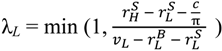, p_H = , p_L = λ_L (v_L − ), yielding gross surplus = π v_H + (1 − π) v_L − (1 − π) max{ v_L − 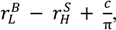0}.

We have found three contracts (in addition to specific performance) that are feasible for the case > : the efficient trade contract, the “no aggrievement” contract of Proposition 2, and, if 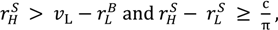, a new “no aggrievement” contract. In general, when > , other contracts may do even better.¹² However, the contracts that we have identified provide a lower bound for what can be achieved.

Proposition 3.

Suppose > and (27). Then an optimal contract yields surplus at least equal to max (v_L, − c, − c, S₃ − c).

Remark: It is easy to check that and so we do not need to include these inequalities as extra conditions in Proposition 3 (see (*)).

We can use Propositions 1 and 3 to see the effect of outside options on surplus. Observe that = S₁, = S₂ when all outside options are zero. Also , are increasing in the seller’s outside options. We may conclude that as in the case the presence of seller outside options increases surplus. The effect of buyer options on surplus is again ambiguous. However, since and S₃ are increasing in these options, and is increasing in them if = , buyer outside options are unambiguously good for surplus when =

Armed with Propositions 2 and 3, let us now turn to the effects of asset ownership. Suppose that there is a fixed set of assets at the disposal of the buyer and the seller, where these assets can be individually or jointly owned. We would expect that the more assets a party owns, and therefore can walk away with if the relationship breaks down, the higher will be that party’s outside option. We might also expect that asset ownership would affect the outside option in the good state more than in the bad state (this is the assumption made in much of the property rights literature). We therefore assume:

(**) If an asset that was previously owned by the buyer, or was jointly owned, now becomes owned by the seller then , and ( − ) rise weakly, and , and ( − ) fall weakly; and vice versa if ownership shifts from the seller to the buyer.

Let’s start with the case where ≡ (that is, = for all asset allocations), and (27) holds. Then Proposition 2 tells us that outside options matter only if the “no aggrievement” contract in (2b) is optimal. In this case it follows from (26) that, keeping − constant, it is optimal to allocate assets to maximize + and, keeping + constant, it is optimal to allocate assets to minimize − . The first goal improves ex post efficiency whereas the second goal helps with investment incentives. According to (**), the second goal is achieved by allocating ownership to the seller. However, it is possible that the buyer has greater use for the assets than the seller if the relationship breaks down in the bad state, in which case the first goal—maximizing + — would be achieved by allocating ownership to the buyer. Thus in general there is a trade-off.

One case where we can make a clear prediction is if an asset is idiosyncratic to the seller: we define this to mean that transferring the asset from the buyer to the seller increases the seller’s outside option without reducing the buyer’s outside option (whatever other assets the buyer and seller own).

Proposition 4.

Assume ≡ and (27). Then it is optimal for the seller to own any asset that is idiosyncratic to her.

Proof.

Compare S₂ with and note that is strictly increasing in .

Proposition 4 implies that joint ownership of an asset (or separate ownership of strictly complementary assets) is suboptimal. An asset that is jointly owned yields a zero outside option for the buyer but would yield a positive outside option for the seller if ownership were transferred to her.

Proposition 4 does not hold generally for the buyer. It may not be optimal for the buyer to own an asset that is idiosyncratic to him (an asset is idiosyncratic to the buyer if transferring the asset from the seller to the buyer increases the buyer’s outside option without reducing the seller’s outside option), given that this may increase − and interfere with the seller’s investment incentives. However, Proposition 4 does extend to the buyer if ≡ (that is, = for all asset allocations).

Proposition 5.

Assume ≡ , (27), and ≡ . Then it is optimal for the seller to own any asset that is idiosyncratic to her and for the buyer to own any asset that is idiosyncratic to him.

Proof. Compare S₂ with and note that is strictly increasing in if they are equal.

Let’s turn now to the case where > . Here less can be said because we have not characterized an optimal contract. However, we know that seller outside options are good for surplus in this case too. Thus, we can make the following observation. Take the view that, if all the assets are jointly owned, then outside options are zero: we are in the situation of Section 2. Now allocate all the assets to the seller. Given (**) the seller’s outside options rise at least weakly and the buyer’s outside options remain at zero. Apply Proposition 3. This tells us that surplus rises (at least weakly) since ≥ S₁ , ≥ S₂.

Thus, we have

Proposition 6.

Assume (27). Start with joint ownership of all assets, where = = = = 0. Then if ownership of each asset is allocated to the seller, surplus rises weakly. Furthermore it rises strictly if > 0, > v_L − and max { − c, − c, S₃ − c} >v_L.

Proof.

It remains only to establish strictness. But this follows from the fact that, if > 0 and > v_L − , and = = 0, the right-hand side of (31), (26) exceeds that of (7), (11), respectively.

Note that the conclusion that seller ownership is better than joint ownership holds also when ≡ , since we already know that in this case seller outside options increase surplus.

Proposition 6 provides some support for the idea, that, taking joint ownership as a starting point, allocating ownership of all the assets to the seller can bring us closer to the first-best. The intuition is that an increase in reduces ex post inefficiency if λ_L < 1, raising (see (26)); and an increase in makes it easier to reward the seller in the good state without causing buyer aggrievement: rises (see (32)). The buyer’s outside options do not change since they were zero under joint ownership and are also zero when the seller owns all the assets. Finally, the new outcome yielding S₃ may become available (see (35)).

Note that Proposition 6 does not establish that seller ownership is optimal. It is possible that buyer ownership is even better. Indeed, we have seen that a change in asset ownership that increases buyer outside options may also increase surplus. All Proposition 6 shows is that seller ownership is better than joint ownership. One case where we can go further is when ≡ . Suppose that shifting ownership of all the assets to the buyer increases his outside option by an amount k in the low state and at least k in the high state, while shifting ownership to the seller increases her outside option by k in the low state and at least k in the high state. (In a sense, asset ownership has an equally powerful effect on the buyer and seller.) Then, it is easily seen from Propositions 2 and 3 that surplus under seller ownership is at least as high as under buyer ownership. Therefore, seller ownership is better than buyer ownership. The intuition is that asset ownership has an extra kick for the seller since it may improve her investment incentives.

It is interesting to compare the results on asset ownership in this section with Hart [16]. In that paper there is no investment and assets are allocated to avoid ex post hold-up, which causes large amounts of aggrievement and shading. It is shown that a party whose payoff is relatively uncertain should own more assets and that a party should own an asset if it is idiosyncratic to him. In the present paper seller incentives replace uncertainty as a driving force and (tend to) push us in the direction of seller ownership. In addition, we saw in the discussion of Proposition 4 that the seller should own assets idiosyncratic to her, but that it may not be optimal for the buyer to own assets idiosyncratic to him to the extent that this interferes with the seller’s investment incentives (it will be optimal for the buyer to own assets idiosyncratic to him if ≡ ).

Of course, the result that the seller should own assets given that her investment is important and that the seller and (under certain assumptions) the buyer should own assets that are idiosyncratic to her or him is also analogous to findings in the standard property rights literature (see, in particular, Hart and Moore [2]).

4. More General Contracts

In this section we show that, for the case where the seller’s outside options are state independent— = r^S, say—the contracts described in Propositions 1 and 2 are optimal among a class of contracts that includes revelation mechanisms.

As in Hart and Moore [11], a (general) contract is a set ∑ of trade-price vectors (λ, p) and a stochastic mapping from a pair of messages β, σ, reported by the buyer and seller, respectively, onto ∑. Since stochastic combinations of (λ, p) vectors are themselves equivalent in payoff terms to (λ, p) vectors (given the risk neutrality of parties), we can write the outcomes of this mechanism in the good and bad states as (λ_H, p_H), (λ_L, p_L), respectively, and suppose that they lie in ∑. (We do not allow for third parties in the contract; we doubt that they would add anything in the present context.)

Each party feels entitled to the best contractual outcome for him subject to the other party realizing some reservation payoff. In the case of voluntary trade, this reservation payoff is the party’s outside option since each party can quit without penalty. However, what is it more generally (e.g., if one party cannot quit at all or can quit only by paying some penalty or must play some other game to determine the quitting price)? Following Hart and Moore [11] we take the view that a party’s reservation payoff is the maximum that the party can achieve from the contract whatever the other party does; where, in the present context, the other party’s actions can include unlimited shading. (The reader may prefer to think of the case where shading is bounded above and the limit is taken as the bound converges to infinity.) In effect, we suppose in the above message game that the first party maximizes his payoff and the second party minimizes the first party’s payoff. Given unlimited shading, the payoff of the first party will be −∞ whenever λ > 0 and will equal his outside option whenever λ = 0.

Since this game is zero-sum it has a unique equilibrium in payoff terms. Player 1’s reservation payoff is his equilibrium payoff in this game. (It might be − ∞.) We can carry out a similar exercise for the second player. This will be a different game since the roles are reversed: player 2 maximizes his payoff while player 1 minimizes player 2’s payoff. Player 2’s reservation payoff is his equilibrium payoff in this game.

Note that a party’s reservation payoff will generally differ from his outside option. For example, under a specific performance contract a party’s outside option is irrelevant.

Denote the seller’s reservation payoff by R^S and the buyer’s by R^B. By assumption the seller’s outside option is state-independent and thus so is R^S. However, the buyer’s reservation payoff can vary with the state and hence we write for the buyer’s reservation payoff in the good state and for his reservation payoff in the bad state.

Armed with these reservation payoffs, we can compute aggrievement levels for the buyer and seller in the two states as follows:

(36)

(37)

where j = H, L denotes the state and ∑ is the convex hull of ∑. The reason for replacing ∑ by its convex hull is that we take the view that if (λ₁, p₁) , (λ₂, p₂) ε∑, and (λ₁,p₁) is below player 1’s reservation level while (λ₂, p₂) is above, then player 2 feels entitled to a convex combination of (λ₁, p₁), (λ₂, p₂) such that player 1’s reservation level is satisfied in expected terms.

An optimal contract, which induces investment, is a choice of ∑ and a message game that maximizes the expected social surplus subject to the investment constraint; that is, which maximizes

(38)

(39)

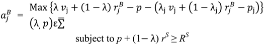
where , , , are given by (36)–(37) and (λ_j, p_j) is an equilibrium of the mechanism in state j, j = H, L.

The proof proceeds by relaxing various constraints and showing that the solution to the relaxed problem can be implemented in such a way that all the original constraints are satisfied. Note first that

p_H + (1 − λ_H) r^S ≥ R^S , p_L + (1 − λ_L) r^S ≥ R^S

(40)

since the seller can always guarantee her (state-independent) reservation level. Thus the buyer feels entitled to (λ_L, p_L) in the good state and (λ_H, p_H) in the bad state. (This is a critical step—it would not be possible if the seller’s outside options varied with the state.) It follows that

(41)

Also

(42)

Consider the relaxed problem in which we replace (36)–(37) by (41)–(42), and choose (λ_H, p_H), (λ_L, p_L) directly, ignoring the constraint that they must be the equilibrium of some mechanism. In other words, we maximize S subject to (39) and (41–42). It is immediate that in the relaxed problem it is optimal to set . Also, if λ_H < 1, S can be raised by increasing λ_H and p_H such that p_H − λ_Hr^S stays constant, since this increases λ_H (v_H − ) − p_H and hence reduces the right-hand side of (41), and does not disturb (39). Hence λ_H = 1. In addition, we always want as low as possible. Hence (41) holds with equality. Finally, if (39) holds strictly, we can increase S by lowering p_H. Hence (39) holds with equality.

We can thus consider the further relaxed problem:

(43)

(44)

(45)

(46)

where the control variables are , , λ_L p_L, p_H.

Case 1: .

Here = 0. Furthermore raising λ_L a little, and adjusting p_H to satisfy (44), increases S. Hence at an optimum λ_L = 1. It follows from the definition of Case 1 that p_H < p_L, but then (44) can hold only if > 0. In this case reducing a little and raising p_H to keep (44) satisfied increases S. Contradiction.

Case 2: .

Again = 0. Combining (44) with the definition of Case 2 yields

(47)

and so

(48)

S is decreasing in λ_L by (16) and so it is optimal to reduce λ_L to the point where either = 0 in (47) or λ_L = 0. But (15) and (17) imply that ≤ 0 if λ_L = 0 .

Hence λ_L will be such that = 0 and we can solve (47) to obtain

(49)

(50)

which corresponds to the “no aggrievement” contract in Proposition 2.

Case 3: .

Now > 0. Using (44) and (45) to solve for and substituting into (43), we can easily see that S is linear in λ_L and .

Moreover,

(51)

(52)

Suppose > 0. Then at an optimum and so (51) implies πθ ≥ (1 − π)(1 − θ). But this means, given (52) and (15), that ≤0.

Hence λ_L = 0 is optimal. However, substituting λ_H = 1, λ_L = 0 in (43) shows that surplus is weakly lower, and strictly lower if > 0, than in the “no aggrievement” contract identified in Case 2. Hence λ_H = 1, λ_L = 0, > 0 cannot be optimal.

We are left with the case where = 0. Since S is linear in λ_L, either λ_L = 0 or λ_L = 1 is optimal (or all 0 ≤ λ_L ≤ 1). We have already argued that λ_H = 1, λ_L = 0 is (weakly) dominated by the “no aggrievement” contract in Case 2. All that remains is λ_H = λ_L = 1. But this is the other contract considered in Proposition 2.

We are left with two candidates for an optimal cntract with investment:

(53)

(54)

Let p_H = v_L − v_L − in the first contract and p_L = λ_L(v_L − ) in the second. Then it is easy to check that the outcomes in (53) and (54) can both be implemented by allowing the seller to choose between (λ_H, p_H) and (λ_L, p_L) at date 1 with the buyer able to say no, i.e., to quit without penalty. For the argument to work in the case of (53) we need to be sure that (20) holds since otherwise the buyer will quit in the good state. However, as noted in Section 3, if the λ_L = λ_H = 1 outcome in (53) is strictly superior to specific performance, then the first inequality in (27) holds. Hence by (27), (20) does indeed hold.

Thus, we have found a mechanism that implements the solution of the relaxed problem. Moreover, it satisfies all the constraints of the original problem, (38)–(39). Therefore, it must solve the original problem. We have thus proved Propositions 1 and 2.

Remark: It is worth considering why this argument does not apply when > . The reason is that in the good state of the world (λ_L, p_L) may be below the seller’s reservation level and so the buyer may not feel entitled to it. However, following our earlier discussion, if (λ_H, p_H) provides the seller with strictly more than her reservation payoff in the good state, the buyer will feel entitled to a convex combination of (λ_H, p_H) and (λ_L, p_L) such that the seller receives her reservation payoff in expected turns. Convexification destroys the linearity that made the above analysis relatively simple, and I have been unable to characterize an optimum in this case. Among other things it is possible that an optimal contract will now consist of more than two trade-price vectors (This may also be a feature of an optimal contract when (27) fails to hold.).

5. Conclusions

In this paper, we have studied a model where the purpose of a long-term contract is to encourage a seller to make a quality-enhancing investment, as well as to achieve ex post efficiency and to avoid shading. We have shown that, if contracts are reference points, the first-best cannot be achieved even when the parties can commit not to renegotiate. We have also shown that asset ownership can increase efficiency.

One obvious question to ask is, what happens if we suppose instead that parties can always renegotiate. This will change the analysis in a number of ways. First, inefficient ex post outcomes, where λ < 1, will no longer be sustainable. Second, certain kinds of (opportunistic) renegotiation may lead to (even) higher levels of aggrievement and shading. Third, the possibility of renegotiation will make it harder to allocate surplus to the seller: even if the seller has the right to make take-it-or-leave-it offers, the buyer can reject the seller’s offer and renegotiate. As Moore and Repullo [22] and Maskin and Tirole [23] have shown, third parties and/or lotteries can help under such conditions. Solving for an optimal contract in the presence of shading, third parties and/or lotteries is a (challenging) topic for future research. However, there seems no reason to think that the main result of this paper—that asset ownership matters—will be overturned.

The model studied in this paper is obviously quite restrictive. We have focused on the case where only one party invests and where the investment is a cross-investment. The reason for the cross-investment assumption is simple. If the investment is a self-investment (the seller’s investment affects her cost but not the buyer’s value) the first-best can be achieved with a specific performance contract since this guarantees efficient trade and ensures that the seller internalizes fully the benefit from her investment. Introducing a second cross-investment by the buyer—the buyer’s investment affects the seller’s cost—would complicate the analysis since we would require more than two states of the world but we suspect that our results—for example, some version of Proposition 5—would generalize. However, analyzing this case must await further research.

References

- Grossman, S.J.; Hart, O. The costs and benefits of ownership: A theory of vertical and lateral integration. J. Polit. Econ. 1986, 94, 691–719. [Google Scholar]
- Hart, O.; Moore, J. Property rights and the nature of the firm. J. Polit. Economy 1990, 98, 1119–1158. [Google Scholar]
- Hart, O. Firms, Contracts, and Financial Structure; Oxford University Press: Oxford, UK, 1995. [Google Scholar]
- Aghion, P.; Holden, R. Incomplete contracts and the theory of the firm: What have we learned over the past 25 years? J. Econ. Perspect. 2011, 25, 181–197. [Google Scholar] [CrossRef]
- Woodruff, C. Non-Contractible investments and vertical integration in the Mexican footwear industry. Int. J. Ind. Organ. 2002, 20, 1197–1224. [Google Scholar] [CrossRef]
- Baker, G.P.; Hubbard, T. Make v. Buy in trucking: Asset ownership, job design and information. Am. Econ. Rev. 2003, 93, 551–572. [Google Scholar] [CrossRef]
- Baker, G.P.; Hubbard, T. Contractibility and asset ownership: On-Board computers and governance in US Trucking. Q. J. Econ. 2004, 119, 1443–1480. [Google Scholar] [CrossRef]
- Acemoglu, D.; Aghion, P.; Griffith, R.; Zilibotti, F. Vertical integration and technology: Theory and evidence. J. Eur. Econ. Assoc. 2010, 8, 2–45. [Google Scholar]
- Gebhardt, G. Does relationship specific investment depend on asset ownership? Evidence from a natural experiment in the housing market. J. Eur. Econ. Assoc. 2013, 11, 201–227. [Google Scholar] [CrossRef]
- Lafontaine, F.; Slade, M. Vertical integration and firm boundaries: The evidence. J. Econ. Lit. 2007, 45, 629–685. [Google Scholar] [CrossRef]
- Hart, O.; Moore, J. Contracts as reference points. Q. J. Econ. 2008, 123, 1–48. [Google Scholar] [CrossRef]
- Fehr, E.; Hart, O.; Zehnder, C. Contracts as reference points – experimental evidence. Am. Econ. Rev. 2011, 101, 493–525. [Google Scholar] [CrossRef]
- Aghion, P.; Fudenberg, D.; Holden, R.; Kunimoto, T.; Tercieu, O. Subgame-Perfect implementation under value perturbations. Q. J. Econ. 2012, 127, 1843–1881. [Google Scholar] [CrossRef]
- Halonen-Akatwijuka, M.; Hart, O. More is less: Why parties may deliberately write incomplete contract. 2013. NBER working paper #19001(submitted). Available online: http://scholar.harvard.edu/hart/publications/more-less-why-parties-may-deliberately-write-incomplete-contracts (accessed on 12 August 2013).
- Fehr, E.; Schmidt, K. Theories of Fairness and Reciprocity: Evidence and Economic Applications. In Advances in Economics and Econometrics: Theory and Applications, Eighth World Congress; Dewatripont, M., Hansen, L.P., Turnovsky, S.J., Eds.; Cambridge University Press: Cambridge, UK, 2003; Volume 1, pp. 208–257. [Google Scholar]
- Hart, O. Hold-up, asset ownership, and reference points. Q. J. Econ. 2009, 124, 267–300. [Google Scholar] [CrossRef]
- Hart, O.; Holmstrom, B. A theory of firm scope. Q. J. Econ. 2010, 125, 483–513. [Google Scholar] [CrossRef]
- MacLeod, W.B.; Malcomson, J. Investments, holdup, and the form of market contract. Am. Econ. Rev. 1993, 83, 811–837. [Google Scholar]
- Che, Y.K.; Hausch, D.B. Cooperative Investments and the Value of Contracting. Am. Econ. Rev. 1999, 89, 125–147. [Google Scholar] [CrossRef]
- Herweg, F.; Schmidt, K. Loss aversion and ex post inefficient renegotiation. 2012. CESifo Work- ing Paper Series No. 4031(submitted). Available online: http://ideas.repec.org/p/ces/ceswps/_4031.html (accessed on 12 August 2013).
- Fehr, E.; Hart, O.; Zehnder, C. How do informal agreements and renegotiation shape contractual reference points? 2012. Harvard University working paper(submitted). Available online: http://scholar.harvard.edu/hart/publications/how-do-informal-agreements-and-renegotiation-shape-contractual-reference-points (accessed on 12 August 2013).
- Moore, J.; Repullo, R. Subgame perfect implementation. Econometrica 1988, 56, 1191–1220. [Google Scholar] [CrossRef]
- Maskin, E.; Tirole, J. Unforeseen contingencies and incomplete contracts. Rev. Econ. Stud. 1999, 66, 83–114. [Google Scholar]
- 3One does not need to go this far, however. See Halonen-Akatwijuka and Hart [14] for an extension.
- 4Shading is a form of negative reciprocity, as studied in the social preferences literature. See, Fehr and Schmidt [15].
- 5In a recent paper, Herweg and Schmidt [20] develop a model of contracts as reference points based on loss aversion rather than aggrievement and shading. Among other things, they show that parties may prefer not to write specific performance contracts but instead to rely on asset ownership to reduce hold-up problems. Herweg and Schmidt’s focus is different from ours. They analyze a situation where renegotiation is required to achieve ex post efficiency, and they do not study general mechanisms or show that asset ownership has a role even when such mechanisms are allowed.
- 6For a further discussion of shading, including examples of buyer and seller shading, see Hart and Moore [11].
- 7Note that we are assuming that the buyer’s entitlement is defined with respect to prices rather than surplus. A buyer might feel that it is reasonable that he pays a higher price if the value of the good is high. It would be interesting to allow for this possibility in extensions of the model. We conjecture that some version of our results will continue to hold as long as the buyer’s perceived fair price does not increase one to one with the value of the good. Of course, if the increase is one to one, that is, the buyer is willing to accept a constant amount of surplus, independent of the quality of the good, the seller becomes the residual claimant and the first-best can be achieved.
- 8One important assumption that we are making implicitly is that the buyer is not aggrieved about the seller’s investment decision per se. If he were then a specific performance contract might cause some shading as a result of the buyer being disappointed that the seller has not invested. One might even imagine that the seller would invest to forestall the buyer becoming angry and shading. Investigating situations where aggrievement is a result of ex ante as well as ex post actions is an interesting topic for future research. See also footnote 7 for a related point.
- 9In the absence of (17), revelation schemes in combination with third parties and/or lotteries may be required to achieve the first-best even when θ = 0.
- 10Note that we suppose that the parties cannot restrict the impact of outside options on payoffs in (12) - (13) except though the choice of λ, e.g., they cannot write exclusive dealing contracts.
- 11In other words, we convexify things. Section 4 does the same thing for general contracts.
- 12As an example, suppose that vH = 20, vL = 14,
![]() = 0,
= 0, ![]() = 0,
= 0, ![]() )= 10,
)= 10, ![]() = 4,
= 4, ![]() , c < 3. The efficient trade contract yields a loss of
, c < 3. The efficient trade contract yields a loss of ![]() relative to the first-best (see (31)). The first “no aggrievement” contract yields a loss of
relative to the first-best (see (31)). The first “no aggrievement” contract yields a loss of ![]() relative to the first-best (see (26)). The second “no aggrievement” contract is not feasible since
relative to the first-best (see (26)). The second “no aggrievement” contract is not feasible since ![]() < vL −
< vL − ![]() . Now consider the following contract: λH = 1, λL = 1, pH = 10, pL =10 − 2c, where the buyer chooses between the two at date 1 and the seller can quit. There is no longer any buyer aggrievement in the good state since the seller’s participation constraint is binding (and there is no buyer aggrievement in the bad state since the buyer gets the lowest possible price). There is no seller aggrievement in the good state because the seller gets the highest possible price. However, there is seller aggrievement in the bad state: the seller receives 10−2c but feels entitled to 10 since this would still satisfy the buyer’s participation constraint. It is easy to see that the seller invests. Gross social surplus is given by S = π vH + (1 − π) vL - π θ (pH − pL) = π vH + (1 − π) vL − θ c. In other words the loss relative to the first-best is θc, which is less than both
. Now consider the following contract: λH = 1, λL = 1, pH = 10, pL =10 − 2c, where the buyer chooses between the two at date 1 and the seller can quit. There is no longer any buyer aggrievement in the good state since the seller’s participation constraint is binding (and there is no buyer aggrievement in the bad state since the buyer gets the lowest possible price). There is no seller aggrievement in the good state because the seller gets the highest possible price. However, there is seller aggrievement in the bad state: the seller receives 10−2c but feels entitled to 10 since this would still satisfy the buyer’s participation constraint. It is easy to see that the seller invests. Gross social surplus is given by S = π vH + (1 − π) vL - π θ (pH − pL) = π vH + (1 − π) vL − θ c. In other words the loss relative to the first-best is θc, which is less than both ![]() and
and ![]() as long as
as long as ![]() .
.
© 2013 by the authors; licensee MDPI, Basel, Switzerland. This article is an open access article distributed under the terms and conditions of the Creative Commons Attribution license (http://creativecommons.org/licenses/by/3.0/).
Share and Cite
Hart, O. Noncontractible Investments and Reference Points. Games 2013, 4, 437-456. https://doi.org/10.3390/g4030437
Hart O. Noncontractible Investments and Reference Points. Games. 2013; 4(3):437-456. https://doi.org/10.3390/g4030437
Chicago/Turabian StyleHart, Oliver. 2013. "Noncontractible Investments and Reference Points" Games 4, no. 3: 437-456. https://doi.org/10.3390/g4030437
APA StyleHart, O. (2013). Noncontractible Investments and Reference Points. Games, 4(3), 437-456. https://doi.org/10.3390/g4030437