Classifying Limited-Move Stability Cycles in 2 × 2 Games

Abstract

The $2\times 2$ game is the simplest non-trivial model of strategic interaction: there are two players, each has two strategies, and each has a strict preference ranking over the four possible outcomes. For models of play that depend only on the ranking of the outcomes, the catalog of $2\times 2$ games permits many useful comparisons and contrasts. By interpreting a $2\times 2$ game as a graph model, we obtain new data on the properties of limited-move ($L_h$) stability. Specifically, for each $2\times 2$ strict ordinal game, we determine the $L_h$-stable outcomes; show how stability depends on the horizon, h; and find the lengths of cycles and the numbers of moves until cycling begins. We then compare our observations with other classifications of these games and with the values of the conflict and harmony indices.

1. Introduction

We must make personal or professional decisions almost daily, often seeking resources to help us with our choices. Each agent’s decisions can affect others, often resulting in a strategic conflict. To make decisions rationally, a decision maker (DM) must define his or her goals and then assess which choices best achieve and balance these goals. Conflict analysis methods can help evaluate possible courses of action by predicting the reactions of others and the eventual outcomes, thus facilitating decision making.

Based on tools from conflict analysis and game theory, Kilgour et al. (1987) proposed a mathematical approach to model and analyze strategic conflicts. The graph model, or Graph Model for Conflict Resolution (GMCR), describes and analyzes patterns of behavior for DMs in strategic conflicts, and is designed to be easy to apply in real-world contexts.

According to the graph model, a conflict is always in one of several possible states; actions by DMs cause the conflict to shift from one state to another. Stability analysis aims to determine, for each state and each DM, whether the DM would choose to move away from that state if it were the current state. A state is stable for a DM who either cannot move away from it or could move away but would choose not to. This choice of moving or not is made in anticipation of the reactions of other DMs to the initial move. The many behavior patterns, or stability definitions, that have been proposed for the graph model are essentially models of the reactions of other DMs as expected by the focal DM. The most common of these stability definitions are listed below, in Section 2.1, with references.

Two particular stability definitions proposed early in the history of the graph model are limited-move stability with horizon h ($L_h$) and non-myopic stability ($NM$) (Kilgour, 1985). The former, $L_h$ stability, the primary topic of this paper, has been recognized as the source of complicated cyclic behavior. Since the latter topic, $NM$ stability, is a limit of $L_h$ stability as h increases without bound, our study in fact sheds light on both of these long-standing but poorly understood stability definitions.

The arena for our study is the set of strict ordinal $2\times 2$ games, as described in the “periodic table” set up by Bruns (2015b), based on the ideas of Robinson and Goforth (2004). The class of games with two players, each with two strategies, and each with a strict ranking of the four possible outcomes, was first identified by Rapoport and Guyer (1966). It is a natural place to study strategic principles that depend only on the ordering of outcomes, such as dominance and pure-strategy Nash equilibria (Brams, 1977; Brams & Kilgour, 2009; Gimon & Leonetti, 2025; Rapoport et al., 1976). It has been rearranged (Brams, 1977) and extended in various directions (Fishburn & Kilgour, 1990; Fraser & Kilgour, 1986; Kilgour & Fraser, 1988); it continues to find interesting uses for other purposes (Omidshafiei et al., 2020).

The notion of limited-move stability takes the positive integer h as a parameter, and assumes that the focal DM anticipates h steps into the future. This DM asks what the final state will be if all DMs make choices to achieve the best final scenario possible for themselves within the h-move horizon, assuming that the preferences of all DMs are common knowledge. Note that each DM’s choices depend only on his or her relative preferences for outcomes—information that is always available in the context of ordinal games.

The main contributions of this work are as follows:

• To explore (see below) the dynamic and oscillatory behavior associated with $L_h$ stability, determining the lengths of cycles and the horizon where cycling emerges for each one of the strictly ordinal $2\times 2$ games;
• To confirm the conjecture of Fang et al. (1993) that, for $2\times 2$ games, all cycles have lengths 1, 2, or 4;
• To compare the classification of 2 × 2 games thus obtained with related classifications in the literature.

There are important ramifications for a number of fields involving bounded rationality and strategic interaction from the study of $2\times 2$ games with a finite horizon. Such analysis provides more realistic decision-making analysis in artificial intelligence and reinforcement learning by modeling and training agents that function under cognitive or computational limitations. These bounded agents are appropriate for real-time systems or situations with constrained processing capacity because they can learn to predict the immediate effects of actions without needing complete solution paths.

In strategic negotiation settings, as in political or diplomatic conflicts, limited-horizon reasoning captures how real-world DMs often make decisions without full foresight, instead relying on short-term planning and heuristics. This is particularly relevant in modeling human negotiations or multi-agent systems where DMs must act under time pressure or informational constraints.

In general, $2\times 2$ limited-horizon game analysis bridges idealized rational models with actual strategic behavior by providing a tractable yet effective method of investigating decision making with bounded foresight. This work is of practical significance in all those domains because it offers a comprehensive knowledge of the cyclic behavior that arises in such analysis.

The concept of limited-move stability originated in the work of Zagare (1984). In that work, $2\times 2$ games are classified according to limited-move equilibria, a closely related concept. However, the analysis is limited to horizons up to 4, what the author calls rules I, II, III, and IV. Moreover, that work classifies games according to whether all or some equilibria remain the same for some or all horizons up to four. The present research considers any finite horizon and observes the cyclic behavior of the whole set of states and not only of the equilibrium states.

This work is organized as follows: In Section 2, a theoretical background about the GMCR and the limited-move stability is presented. Section 3 contains the main findings of this work, which is the determination of lengths of cycles and the horizon where cycles begin in all $2\times 2$ strictly ordinal games. A comparison with other results in the literature is made in Section 4. Finally, Section 5 concludes the paper by summing up the contributions and questions for future works. The definitions of all symbols and abbreviations used in the manuscript can be found in “Symbols and Abbreviations” at the end of the conclusions.

2. Theoretical Background

2.1. Graph Model for Conflict Resolution

The Graph Model for Conflict Resolution (GMCR) (Kilgour et al., 1987) is a flexible mathematical tool designed to model and analyze the interactions of DMs through their possible moves and countermoves. Formally, a graph model has the following several components:

• The set N of all DMs acting in the conflict;
• The set S of all feasible states of the conflict, generally consisting of all possible combinations of actions that the DMs can take;
• For each DM $i\in N$, a loop-free directed graph, $D_i=(S,A_i)$, where the set of nodes (common to all DMs’ graphs) is S, the set of states, and $A_i\subseteq S\times S$ specifies the state transitions controlled by DM i;
• For each DM $i\in N$, a preference structure on S that is usually taken to be an asymmetric ir-reflexive binary relation, denoted by ${\succ }_i$, where, for states $s,t\in S$, $s{\succ }_{i}t$ means that DM i strictly prefers state s to state t.

In GMCR, accessibility is often represented by sets of unilateral moves (UMs), represented by $R_i\left(s\right)\subseteq S-\left\{s\right\}$, where a state belongs to $R_i\left(s\right)$ if it can be accessed by DM i, from state s, in a single step. Formally, the definition is $R_i\left(s\right)=\{t\in S:(s,t)\in A_i\}$.

Together, DMs, states, accessibility relations, and preferences constitute a model of a conflict. The next step, stability analysis, predicts which states are possible outcomes. Specifically, this analysis verifies, for each state of the conflict, which DMs would be willing to move away from the state (if it were the current state). In the GMCR literature, there are many stability definitions that describe the interests of DMs in moving away from a state. Effectively, they are models of DMs’ strategic behavior in conflict situations. In all of these definitions, stability is analyzed from the point of view of a single DM, called the focal DM. A state that is stable according to a particular stability notion for every DM in the graph model is called an equilibrium under that stability definition.

The most commonly used stability definitions are those of Nash (1950), general metarationality (GMR) (Howard, 1971), symmetric metarationality (SMR) (Howard, 1971), sequential stability (SEQ) (Fraser & Hipel, 1984), and symmetric sequential stability (SSEQ) (Rêgo & Vieira, 2017). Intuitively, in Nash stability, the focal DM, ignoring the possible reactions of opponents, chooses to move if and only if a preferable state is reached. In $GMR$ and $SEQ$ stabilities, the focal DM asks whether opponents can sanction the initial move by taking the conflict to a state that the focal DM does not prefer to the initial state. These concepts differ in that, under SEQ, the opponents react only with improvements, while under GMR, sanctions are not necessarily improvements for the sanctioner. Thus, SEQ stability is stronger in the sense that both the initial move and the sanction must be “credible”; under GMR, this adjective applies only to the initial move. In the SMR and SSEQ concepts, the focal DM analyzes the possible responses of the opponents, exactly as with GMR and SEQ, but in addition, the focal DM also asks whether the sanction can be escaped by a further move—that is, whether a state preferable to the initial state can be reached in three moves. Like GMR, SMR allows non-credible sanctions; like SEQ, SSEQ insists that sanctions be credible. All these stability definitions have a common feature: each allows a fixed number of moves and countermoves—1, 2, or 3—and thus has a fixed horizon.

An early stability notion that can be used with any horizon is limited-move stability ($L_h$). It specifies that the focal DM decides whether to move by considering the final state that would be reached after a maximum of h moves, assuming that other DMs make choices to achieve the best final outcome for themselves. Of course, final outcomes, and $L_h$ stabilities, may change as h changes. In fact, oscillatory and periodic behavior has been noted in some cases, even when all DMs anticipate the same final state if the horizon is long enough Fang et al. (1993).

In this paper, we are particularly interested in identifying the length and the initial horizon of cycles in $L_h$ stability in graph models obtained from $2\times 2$ games. We interpret each outcome as a state, and preserve the accessibility relation inherent in the original game. We next describe the notion of $L_h$ stability in detail, for the context of graph models with $\left|N\right|=2$ DMs, where $|·|$ represents the cardinality of a set.

2.2. Limited Move Stability

In $L_h$ stability, DMs are allowed to perform a maximum of h actions and counteractions. In this concept, the focal DM anticipates, h steps ahead, what the final state of the conflict will be, considering that decision makers always change their actions in order to reach the best possible scenario for themselves, and that the preferences of all DMs are common knowledge.

Our approach is to assume that each DM has preferences on S that are complete, transitive, and asymmetric. To work with this concept, let $K_i\left(s\right)$ be the cardinality of the set of states that are less preferred than state s for DM i. Formally, we have that $K_i\left(s\right)=\left|\left\{t\in S:s{\succ }_{i}t\right\}\right|$. For $i\in N$, $s\in S$, and $h=0,1,\dots$, $G_h(i,s)\in S$ is the state that DM i anticipates will be the final state of the conflict if the conflict starts in state s, DM i moves first, DMs alternate moves, at most h moves are made, and each DM chooses its moves so as to achieve the best final state for itself and expects the other DM to do likewise. By convention, $G_0(·,s)=s$ and, for $h\ge 1$, $G_h(i,s)$ is constructed recursively as follows:

$$\begin{array}{l}{G}_h(i,s)=\left\{\begin{array}{cc}s,\hfill & \mathrm{if}{R}_i\left(s\right)=\varnothing \hfill \\ s,\hfill & \mathrm{if}{K}_i\left(s\right)\ge A_h(i,s)\hfill \\ G_{h-1}(j,M_h(i,s)),\hfill & \mathrm{otherwise},\hfill \end{array}\right.\end{array}$$

where $M_h(i,s)\in argmax\{K_i\left(G_{h-1}(j,t)\right):t\in R_i\left(s\right),j\ne i\}$ and

$$A_h(i,s)=K_i\left(G_{h-1}(j,M_h(i,s))\right).$$

Intuitively, the anticipated state $G_h(i,s)$ will be equal to s if DM i cannot move away from s or if s is at least as preferred as the most preferred state $G_{h-1}(j,M_h(i,s))$ that can be anticipated at horizon $h-1$ by DM i when DM i moves away from state s and its opponent responds, with horizon $h-1$. Otherwise, $G_h(i,s)=G_{h-1}(j,M_h(i,s))$. It is worth pointing out that, in the case of conflicts described by $2\times 2$ games, $M_h(i,s)$ is always equal to the unique element in $R_i\left(s\right)$, since $R_i\left(s\right)$ is always a singleton set.

Note that, in the limited-move stability concept, not only are DMs’ preferences over states common knowledge, but also it is common knowledge that all DMs make moves that are most beneficial to themselves at each horizon $h^{\prime }<h$. Figure 1 provides a step-by-step flowchart to calculate the final anticipated state $G_h(i,s)$. The formal definition of limited-move ($L_h$) stability is as follows:

Figure 1. Step-by-step flowchart to calculate $G_h(i,s)$.

Figure 1. Step-by-step flowchart to calculate $G_h(i,s)$.

Definition 1 

(Kilgour, 1985). A state $s\in S$ is ($L_h$) stable for DM $i\in N$, or stable according to the limited-move stability concept with horizon h, if and only if $G_h(i,s)=s$.

We refer the reader to the examples described in Section 3 for a better understanding of the $L_h$ stability and all the notation defined in this section.

2.3. Cycles in $L_h$ Stability

Cycles in $L_h$ stability are periodic or oscillatory trajectories as a function of the horizon h that arise in the dynamical system, considering the $L_h$ stability properties. This implies that, even if the system may have a stable equilibrium point $L_h$, it may also present periodic or oscillatory dynamical behaviors when the horizon of analysis h varies.

Formally, Definition 2 establishes the meaning of a cycle in the $L_h$ stability.

Definition 2 

(Fang et al., 1993). A game enters a cycle of length r, starting from horizon h, if $G_{t+r}(i,s)=G_t(i,s)$, for every integer t such that $t\ge h$, all $i\in N$, and all $s\in S$, with h and r being the smallest integers with this property.

Note that, by the definition of $L_h$ stability, $G_t(i,s)$ is the state that DM i anticipates as the final state when the initial state is s and the horizon is t. If the model enters a cycle of length r at horizon h, then, for any number of increments of size r in the horizon, each DM anticipates the same final state from any initial state. For example, in a game that presents a cycle of length 2, if the horizon is large enough, then whenever the horizon is increased by 2, the anticipated states will be the same for all DMs from all states of the conflict.

A game that has a cycle of length 1 is said to have a fixed point. However, cycles of other lengths are possible. Fang et al. (1993) stated that, of all the games analyzed so far, only cycles of length 1, 2, or 4 had been encountered, and conjectured that these are the only possibilities. In this work, our main objective is to investigate cycles in all $2\times 2$ games and identify the cycle length and the horizon at which cycles begin.

2.4. $2\times 2$ Strict Ordinal Games

The class of games with two players, each with two strategies and no indifference among the four outcomes, was first identified by Rapoport and Guyer (1966). It can be categorized into 12 distinct payoff patterns for each DM. This classification derives from the fact that there are $24=4!$ permutations of the numbers 1 through 4, which we divide by two so as to identify those that are distinct only due to the names of the DMs’ strategies. For example, describing the Prisoners’ Dilemma with “Defection” on the top line and “Cooperation” on the bottom (reversing those strategies) does not change the game in any essential way. These 12 patterns are named according to the names of the symmetric games that they generate: No Conflict/Concord (Nc), Harmony (Ha), Peace (Pc), Coordination (Co), Assurance (As), Stag-Hunt (Sh), Prisoners’ Dilemma (Pd), Deadlock/Anti-Prisoners’ Dilemma (Dl), Compromise/Anti-Chicken (Cm), Hero (Hr), Battle of the Sexes (Ba), and Chicken (Ch).

Thus, in principle, there are 144 strictly ordinal $2\times 2$ games. However, if both DMs switch roles, the conflict does not change, generating a symmetry. In fact, there are 12 symmetric games in which both DMs have the same pattern of behavior (such as the Prisoners’ Dilemma, Chicken game, Stag-Hunt, etc). For each of the remaining 132 games, where DMs have different behavioral patterns, there is a symmetric one where the behavioral patterns of the DMs are reversed. For example, one DM playing the Chicken game and the other playing the Prisoners’ Dilemma (ChPd) is the same game (PdCh), where the roles of the DMs are reversed. Thus, they share the same result in any strategic analysis, and consequently, there is no need for duplication, only repetition of the results found. By dividing the 132 distinct games by two, we obtain 66, which added to the other 12 symmetric games’ result in the 78 distinct $2\times 2$ games that were analyzed according to the $L_h$ cycle.

3. ${\mathit{L}}_{\mathit{h}}$ Cycles in $\mathbf{2}\times \mathbf{2}$ Games

We analyze each of the 78 distinct $2\times 2$ games for their $L_h$ cycle. Example 1 illustrates our methodology with an example of a game that enters into a cycle of length 2 from horizon $h=2$.

Example 1. 

To illustrate the concept of cycles in the stability $L_h$, consider the game BaCo, of which the normal form is displayed in

Table 1. Normal form of the BaCo game.

	DM j
DM i	(3,1)	(2,4)
	(1,3)	(4,2)

.

The game BaCo is the one in which the utilities of the row player are according to the Battle of the sexes game and those of the column player are according to the Coordination game.

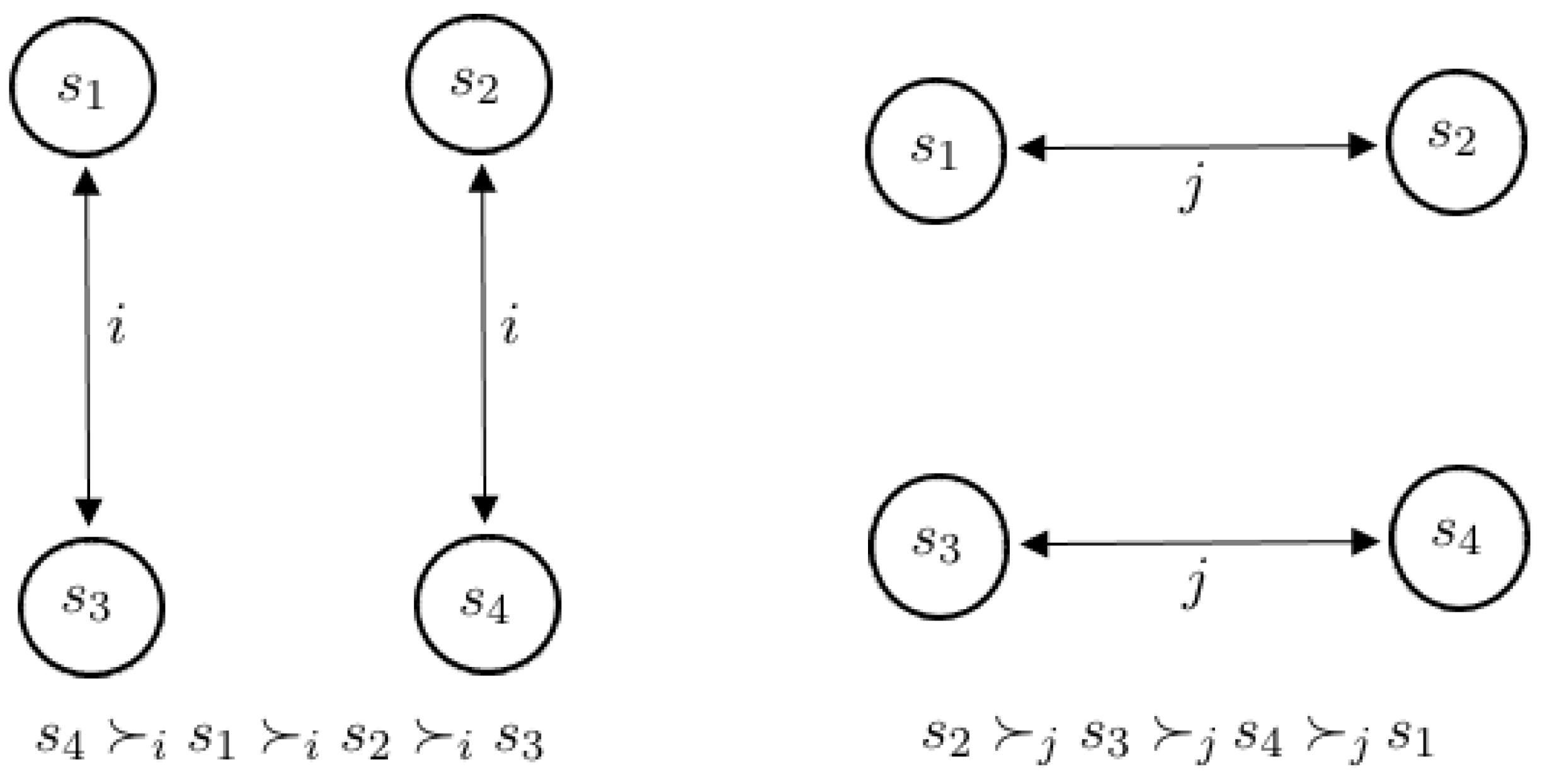
This game can be treated as a graph model. By convention, we will use $s_1$ and $s_2$ to represent the states of the cells in the first row and $s_3$ and $s_4$ to represent the states of the cells in the second row. We will call the DMs of this game DM i and DM j. Note that since DM i can alter their position in the conflict by switching rows, and DM j can do so by switching columns, the graph model representing this conflict, along with the DMs’ preferences over the conflict states, appears in Figure 2. Since this same convention is used for all $2\times 2$ games, it follows that, for any given $s\in S$, the sets $R_i\left(s\right)$ and $R_j\left(s\right)$ are the same in all games. Consequently, for any given $s\in S$, the value of the function $M_h(i,s)\in R_i\left(s\right)$ is the same for every horizon and every $2\times 2$ game, as it can be seen in the tables of Examples 1 and 2.

For didactic purposes, before studying the problem of cycles in this example, we illustrate how to analyze the limited-move stability of state $s_1$ for DM i considering a horizon $h=5$. Figure 3 displays a tree with all sequence of alternate moves that DMs i and j can make starting from a move of DM i from state $s_1$ and considering at most five moves in the sequence. To obtain the anticipate the final state $G_5(i,s_1)$, we need to analyze first the final moves of the DMs. In this example, the final move that can be made is a move from DM i considering horizon 1 from state $s_1$. Since $R_i\left(s_1\right)=\left\{s_3\right\}$, it follows that $M_1(i,s_1)=s_3$ and $A_1(i,s_1)=K_i\left(s_3\right)=0$. As $K_i\left(s_1\right)=2>0=A_1(i,s_1)$, we have that $G_1(i,s_1)=s_1$. Moving one step above, from state $s_2$, DM j can only move to $s_1$ and anticipates that the conflict will end in $s_1$ because $G_1(i,s_1)=s_1$. Thus, it follows that $M_2(j,s_2)=s_1$ and $A_2(j,s_2)=K_j\left(G_1(i,M_2(j,s_2))\right)=K_j\left(G_1(i,s_1)\right)=K_j\left(s_1\right)=0$. As $K_j\left(s_2\right)=3>0=A_2(j,s_2)$, it follows that $G_2(j,s_2)=s_2$. Continuing one more step above in the tree, from state $s_4$, DM i can only move to $s_2$ and anticipates that the conflict will end in $s_2$ because $G_2(j,s_2)=s_2$. Thus, it follows that $M_3(i,s_4)=s_2$ and $A_3(i,s_4)=K_i\left(G_2(j,M_3(i,s_4))\right)=K_i\left(G_2(j,s_2)\right)=K_i\left(s_2\right)=1$. As $K_i\left(s_4\right)=3>1=A_3(i,s_4)$, it follows that $G_3(i,s_4)=s_4$. Going one more step above in the tree, we have that, from state $s_3$, DM j can only move to $s_4$ and anticipates that the conflict will end in $s_4$ because $G_3(i,s_4)=s_4$. Thus, it follows that $M_4(j,s_3)=s_4$ and $A_4(j,s_3)=K_j\left(G_3(i,M_4(j,s_3))\right)=K_j\left(G_3(i,s_4)\right)=K_j\left(s_4\right)=1$. As $K_j\left(s_3\right)=2>1=A_4(j,s_3)$, it follows that $G_4(j,s_3)=s_3$. Finally, at the initial move of DM i from $s_1$, we have that DM i can only move to $s_3$ and anticipates that the conflict will end in $s_3$ because $G_4(j,s_3)=s_3$. Thus, it follows that $M_5(i,s_1)=s_3$ and $A_5(i,s_1)=K_i\left(G_4(j,M_5(i,s_1))\right)=K_i\left(G_4(j,s_3)\right)=K_i\left(s_3\right)=0$. As $K_i\left(s_1\right)=2>0=A_5(i,s_1)$, it follows that $G_5(i,s_1)=s_1$, which implies that state $s_1$ is $L_5$ stable for DM i.

We will use the procedure described above to analyze the $L_h$ stability of the states for values $h=1,2,3,4,5$. Considering $h=1$, we present in

Table 2. Stability analysis $L_1$ in BaCo game.

State	${\mathit{s}}_{\mathbf{1}}$	${\mathit{s}}_{\mathbf{2}}$	${\mathit{s}}_{\mathbf{3}}$	${\mathit{s}}_{\mathbf{4}}$
DM i
$A_1(i,·)$	0	3	2	1
$M_1(i,·)$	$s_3$	$s_4$	$s_1$	$s_2$
$G_1(i,·)$	$s_1$	$s_4$	$s_1$	$s_4$
DM j
$A_1(j,·)$	3	0	1	2
$M_1(j,·)$	$s_2$	$s_1$	$s_4$	$s_3$
$G_1(j,·)$	$s_2$	$s_2$	$s_3$	$s_3$

the results of the $L_1$ stability analysis for both DMs of the conflict. Note that states $s_1$ and $s_4$ are $L_1$ stable for DM i and states $s_2$ and $s_3$ are $L_1$ stable for DM j.

Considering now $h=2$,

Table 3. Stability analysis $L_2$ in BaCo game.

State	${\mathit{s}}_{\mathbf{1}}$	${\mathit{s}}_{\mathbf{2}}$	${\mathit{s}}_{\mathbf{3}}$	${\mathit{s}}_{\mathbf{4}}$
DM i
$A_2(i,·)$	0	0	1	1
$M_2(i,·)$	$s_3$	$s_4$	$s_1$	$s_2$
$G_2(i,·)$	$s_1$	$s_2$	$s_2$	$s_4$
DM j
$A_2(j,·)$	1	0	1	0
$M_2(j,·)$	$s_2$	$s_1$	$s_4$	$s_3$
$G_2(j,·)$	$s_4$	$s_2$	$s_3$	$s_4$

presents the results of the $L_2$ stability analysis for DMs i and j. Note that states $s_1$, $s_2$, and $s_3$ are $L_2$ stable for DM i and states $s_2$, $s_3$, and $s_4$ are $L_2$ stable for DM j.

Now, considering $h=3$,

Table 4. Stability analysis $L_3$ in BaCo game.

State	${\mathit{s}}_{\mathbf{1}}$	${\mathit{s}}_{\mathbf{2}}$	${\mathit{s}}_{\mathbf{3}}$	${\mathit{s}}_{\mathbf{4}}$
DM i
$A_3(i,·)$	0	3	3	1
$M_3(i,·)$	$s_3$	$s_4$	$s_1$	$s_2$
$G_3(i,·)$	$s_1$	$s_4$	$s_4$	$s_4$
DM j
$A_3(j,·)$	3	0	1	3
$M_3(j,·)$	$s_2$	$s_1$	$s_4$	$s_3$
$G_3(j,·)$	$s_2$	$s_2$	$s_3$	$s_2$

presents the results of the $L_3$ stability for DMs i and j. We have that states $s_1$, $s_4$, and $s_3$ are $L_3$ stable for DM i, while states $s_2$ and $s_3$ are $L_3$ stable for DM j.

Considering $h=4$,

Table 5. Stability analysis $L_4$ in BaCo game.

State	${\mathit{s}}_{\mathbf{1}}$	${\mathit{s}}_{\mathbf{2}}$	${\mathit{s}}_{\mathbf{3}}$	${\mathit{s}}_{\mathbf{4}}$
DM i
$A_4(i,·)$	0	1	1	1
$M_4(i,·)$	$s_3$	$s_4$	$s_1$	$s_2$
$G_4(i,·)$	$s_1$	$s_2$	$s_2$	$s_4$
DM j
$A_4(j,·)$	1	0	1	1
$M_4(j,·)$	$s_2$	$s_1$	$s_4$	$s_3$
$G_4(j,·)$	$s_4$	$s_2$	$s_3$	$s_4$

presents the results of the $L_4$ stability for i and j. Note that $s_1$, $s_2$, and $s_4$ are $L_4$ stable for DM i, while states $s_2$, $s_3$, and $s_4$ are $L_4$ stable for DM j. Note also that this is the same result obtained in the $L_2$ stability analysis.

Considering now $h=5$,

Table 6. Stability analysis $L_5$ in BaCo game.

State	${\mathit{s}}_{\mathbf{1}}$	${\mathit{s}}_{\mathbf{2}}$	${\mathit{s}}_{\mathbf{3}}$	${\mathit{s}}_{\mathbf{4}}$
DM i
$A_5(i,·)$	0	3	3	1
$M_5(i,·)$	$s_3$	$s_4$	$s_1$	$s_2$
$G_5(i,·)$	$s_1$	$s_4$	$s_4$	$s_4$
DM j
$A_5(j,·)$	3	0	1	3
$M_5(j,·)$	$s_2$	$s_1$	$s_4$	$s_3$
$G_5(j,·)$	$s_2$	$s_2$	$s_3$	$s_2$

presents the results of the $L_5$ stability for DMs i and j. We have that states $s_1$ and $s_4$ and $s_3$ are $L_5$ stable for DM i, while states $s_2$ and $s_3$ are $L_5$ stable for DM j. Note also that this is the same result obtained in the $L_3$ stability analysis.

From the tables, we can see that, starting at horizon $h=2$, the BaCo game enters a cycle of length 2, i.e., the state anticipated by DM i (resp., DM j), from a state $s\in \{s_1,s_2,s_3,s_4\}$, considering that a horizon $t+2$ is the same state anticipated, from s, considering a horizon t, for every integer $t\ge 2$.

Example 2 discusses the analysis of a game that has a fixed point (cycle of length 1) from horizon $h=5$.

Example 2. 

In this example, we consider the ChAs game, whose normal form is presented in

Table 7. Normal form of the ChAs game.

	DM j
DM i	(2,2)	(3,4)
	(1,3)	(4,1)

. Analogously to Example 1, this game can be represented as a graph model in which the states, DMs, and accessibility relations are identical to those in Figure 2, except for the preference orderings of the DMs. Specifically, the preferences are now given by $s_4{\succ }_i{s}_2{\succ }_i{s}_1{\succ }_i{s}_3$ for DM i, and $s_2{\succ }_j{s}_3{\succ }_j{s}_1{\succ }_j{s}_4$ for DM j.

Following the same procedure as in the previous example, we now examine the $L_h$ stability of the states in the ChAs game for horizons $h=1,2,3,4,5,6$. We begin with $h=1$.

Table 8. Stability analysis $L_1$ in ChAs game.

State	${\mathit{s}}_{\mathbf{1}}$	${\mathit{s}}_{\mathbf{2}}$	${\mathit{s}}_{\mathbf{3}}$	${\mathit{s}}_{\mathbf{4}}$
DM i
$A_1(i,·)$	0	3	1	2
$M_1(i,·)$	$s_3$	$s_4$	$s_1$	$s_2$
$G_1(i,·)$	$s_1$	$s_4$	$s_1$	$s_4$
DM j
$A_1(j,·)$	3	1	0	2
$M_1(j,·)$	$s_2$	$s_1$	$s_4$	$s_3$
$G_1(j,·)$	$s_2$	$s_2$	$s_3$	$s_3$

reports the results of the $L_1$ stability analysis for both DMs in the conflict. Note that states $s_1$ and $s_4$ are $L_1$-stable for DM i, while states $s_2$ and $s_3$ are $L_1$-stable for DM j.

For $h=2$, the results of the $L_2$ stability analysis for DMs i and j are summarized in

Table 9. Stability analysis $L_2$ in ChAs game.

State	${\mathit{s}}_{\mathbf{1}}$	${\mathit{s}}_{\mathbf{2}}$	${\mathit{s}}_{\mathbf{3}}$	${\mathit{s}}_{\mathbf{4}}$
DM i
$A_2(i,·)$	0	0	2	2
$M_2(i,·)$	$s_3$	$s_4$	$s_1$	$s_2$
$G_2(i,·)$	$s_1$	$s_2$	$s_2$	$s_4$
DM j
$A_2(j,·)$	0	1	0	1
$M_2(j,·)$	$s_2$	$s_1$	$s_4$	$s_3$
$G_2(j,·)$	$s_1$	$s_2$	$s_3$	$s_1$

. It can be observed that states $s_1$, $s_2$, and $s_4$ are $L_2$-stable for DM i, whereas states $s_2$ and $s_3$ are $L_2$-stable for DM j.

To the case $h=3$,

Table 10. Stability analysis $L_3$ in ChAs game.

State	${\mathit{s}}_{\mathbf{1}}$	${\mathit{s}}_{\mathbf{2}}$	${\mathit{s}}_{\mathbf{3}}$	${\mathit{s}}_{\mathbf{4}}$
DM i
$A_3(i,·)$	0	1	1	2
$M_3(i,·)$	$s_3$	$s_4$	$s_1$	$s_2$
$G_3(i,·)$	$s_1$	$s_2$	$s_1$	$s_4$
DM j
$A_3(j,·)$	3	1	0	3
$M_3(j,·)$	$s_2$	$s_1$	$s_4$	$s_3$
$G_3(j,·)$	$s_2$	$s_2$	$s_3$	$s_2$

reports the outcomes of the $L_3$ stability analysis for DMs i and j. In this setting, states $s_1$, $s_2$, and $s_4$ are $L_3$-stable for DM i, whereas states $s_2$ and $s_3$ are $L_3$-stable for DM j.

For the horizon $h=4$, the outcomes of the $L_4$ stability evaluation for DMs i and j are displayed in

Table 11. Stability analysis $L_4$ in ChAs game.

State	${\mathit{s}}_{\mathbf{1}}$	${\mathit{s}}_{\mathbf{2}}$	${\mathit{s}}_{\mathbf{3}}$	${\mathit{s}}_{\mathbf{4}}$
DM i
$A_4(i,·)$	0	2	2	2
$M_4(i,·)$	$s_3$	$s_4$	$s_1$	$s_2$
$G_4(i,·)$	$s_1$	$s_2$	$s_2$	$s_4$
DM j
$A_4(j,·)$	3	1	0	1
$M_4(j,·)$	$s_2$	$s_1$	$s_4$	$s_3$
$G_4(j,·)$	$s_2$	$s_2$	$s_3$	$s_1$

. In this case, states $s_1$, $s_2$, and $s_4$ are $L_4$-stable for DM i, whereas states $s_2$ and $s_3$ are $L_4$-stable for DM j.

When the horizon is to $h=5$, the $L_5$ stability outcomes for DMs i and j are reported in

Table 12. Stability analysis $L_5$ in ChAs game.

State	${\mathit{s}}_{\mathbf{1}}$	${\mathit{s}}_{\mathbf{2}}$	${\mathit{s}}_{\mathbf{3}}$	${\mathit{s}}_{\mathbf{4}}$
DM i
$A_5(i,·)$	0	1	2	2
$M_5(i,·)$	$s_3$	$s_4$	$s_1$	$s_2$
$G_5(i,·)$	$s_1$	$s_2$	$s_2$	$s_4$
DM j
$A_5(j,·)$	3	1	0	3
$M_5(j,·)$	$s_2$	$s_1$	$s_4$	$s_3$
$G_5(j,·)$	$s_2$	$s_2$	$s_3$	$s_2$

. In this case, states $s_1$, $s_2$, and $s_4$ are $L_5$-stable for DM i, whereas states $s_2$ and $s_3$ are $L_5$-stable for DM j.

Finally, for horizon $h=6$,

Table 13. Stability analysis $L_6$ in ChAs game.

State	${\mathit{s}}_{\mathbf{1}}$	${\mathit{s}}_{\mathbf{2}}$	${\mathit{s}}_{\mathbf{3}}$	${\mathit{s}}_{\mathbf{4}}$
DM i
$A_6(i,·)$	0	2	2	2
$M_6(i,·)$	$s_3$	$s_4$	$s_1$	$s_2$
$G_6(i,·)$	$s_1$	$s_2$	$s_2$	$s_4$
DM j
$A_6(j,·)$	3	1	0	3
$M_6(j,·)$	$s_2$	$s_1$	$s_4$	$s_3$
$G_6(j,·)$	$s_2$	$s_2$	$s_3$	$s_2$

presents the outcomes of the $L_6$ stability analysis for DMs i and j. In this scenario, states $s_1$, $s_2$, and $s_4$ are $L_6$-stable for DM i, while states $s_2$ and $s_3$ are $L_6$-stable for DM j. It is worth noting that all anticipated states for both DMs considering a horizon $h=6$ are identical to those observed considering the horizon $h=5$. Moreover, since, by definition, the anticipated state considering a horizon h only depends on the anticipated states that consider an immediately previous horizon; for all $h>6$, the anticipated states will continue to be the same. Thus, the analysis enters into a cycle of length 1 from horizon $h=5$. Finally, it is also worth pointing out that, although the cycle of anticipated states only begins at $h=5$, the same sets of stable states are obtained since $h=2$ for both DMs.

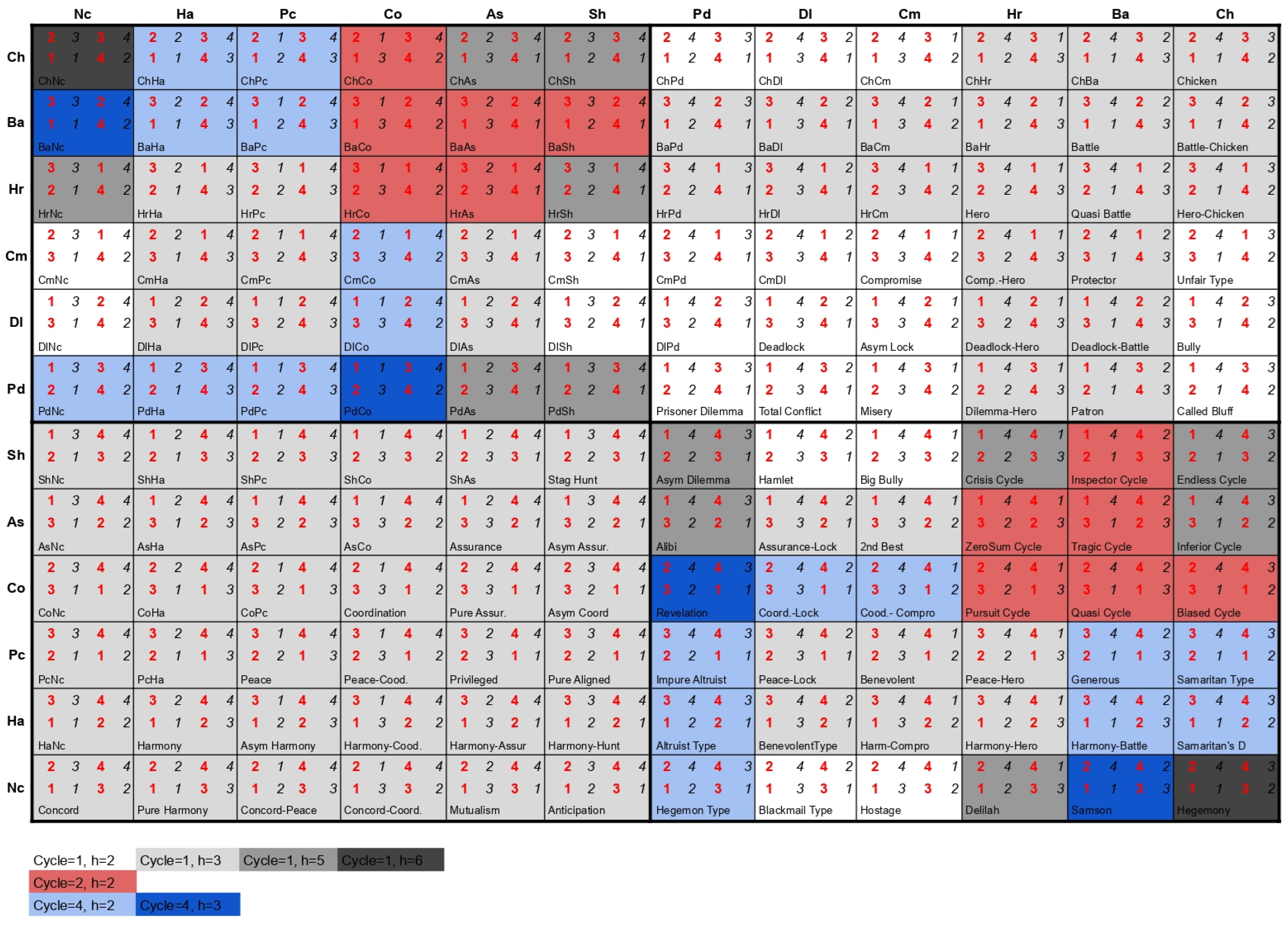
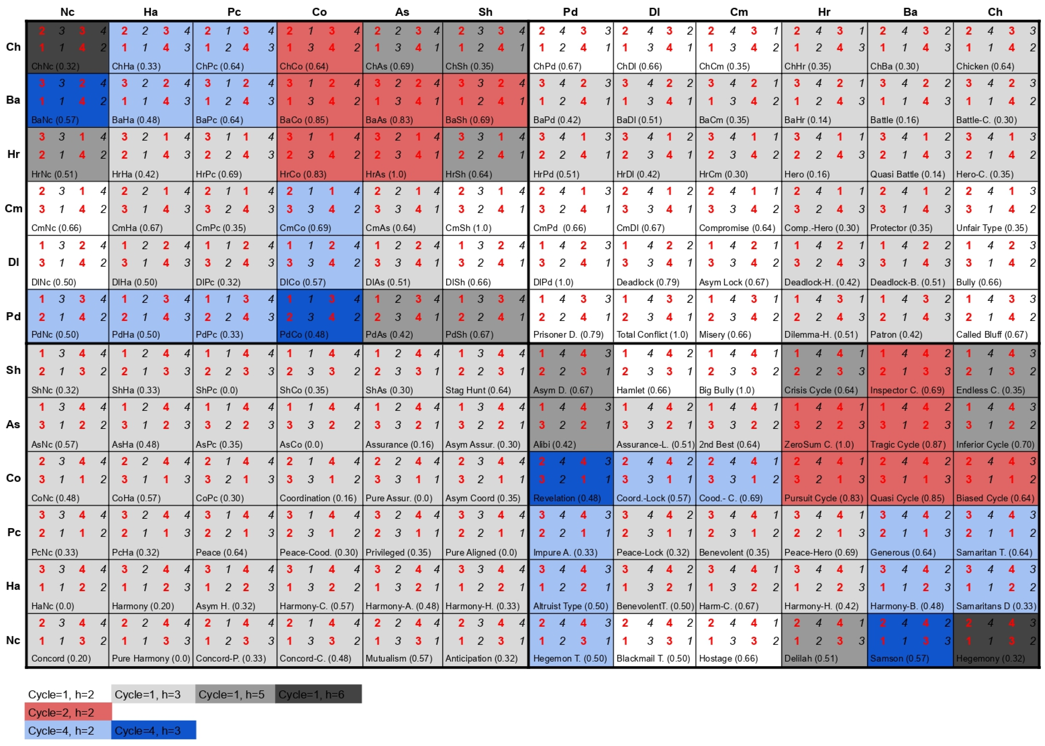
In Figure 4, we present the ordinal utilities of all 144 $2\times 2$ games organized in the same way as in Bruns (2015a) (which is also replicated here in Figure 5). In Figure 4 (and in all other figures that follow), the utilities of the row DM are highlighted in red, while those of the column DM are in black. Each cell in those figures describes one $2\times 2$ game and contains the utilities for both DMs according to the behavioral patterns described in the row and in the column of the cell.

Moreover, in Figure 4, we highlight with the same colors the games with the same resulting cycle lengths, and the horizon in which the cycle begins is highlighted by shades of the color of that cycle, with horizon $h=2$ being the weakest shade and $h=6$ being the strongest shade. As it can be seen, indeed, for all $2\times 2$ games, only cycles of lengths 1, 2, and 4 occur, as it was conjectured by Fang et al. (1993). A cycle of length 1 can begin at horizon $h=2, 3, 5$, or 6, while cycles of length 2 only begin at horizon $h=2$, and cycles of length 4 can start at either $h=2$ or $h=3$. The results displayed in Figure 4 determine for each $2\times 2$ game the maximum horizon that needs to be analyzed according the $L_h$ stability since, for each one of these games, the $L_h$ stability analysis enters into a cyclic behavior, not being necessary to analyze it for higher horizons. For example, the games in dark blue in Figure 4 only need to be analyzed up to horizon 6, since it enters into a cycle of length 4 from $h=3$.

4. Related Work

There are many works that propose classification or scores for $2\times 2$ games. In this section, we related our classification with those of Bruns (2015a) and Omidshafiei et al. (2020). Moreover, we also analyze how the harmony index (Zizzo, 2002) and conflict index (Gimon & Leonetti, 2025) vary according to our classification.

4.1. Brun’s Classification Based on the Pure Nash Equilibria of the Games

Changes in utilities can transform, for example, the Prisoner’s Dilemma game into the Stag-Hunt game; that is, changes in utilities can transform one game into another. Based on this view, Bruns (2015a) demonstrated how a topology of exchanges of utilities can elegantly organize the $2\times 2$ games in a periodic table, structured in a natural order according to the exchange neighbors, the alignment of the best outcomes, the symmetry, the number of dominant strategies and equilibria, among other properties. According to Bruns (2015a), this representation visually further shows the topology of $2\times 2$ games, showing the relationships between games and the ways to transform strategic situations. Furthermore, they present the diversity of $2\times 2$ games, the variety of strategic situations in which the outcome of each person’s action depends on what the other decides, and the range of possible incentive structures when two people have two interdependent choices.

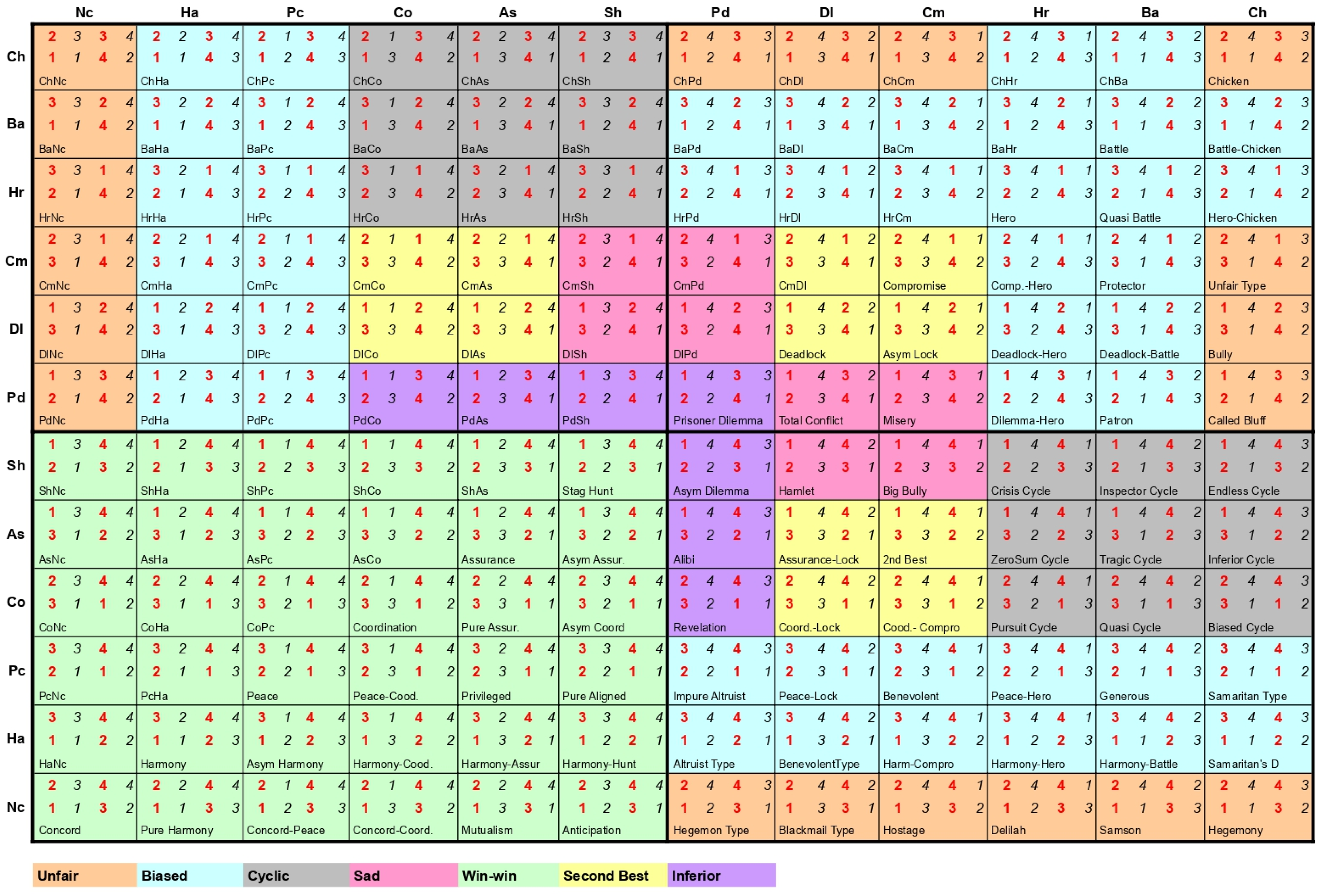
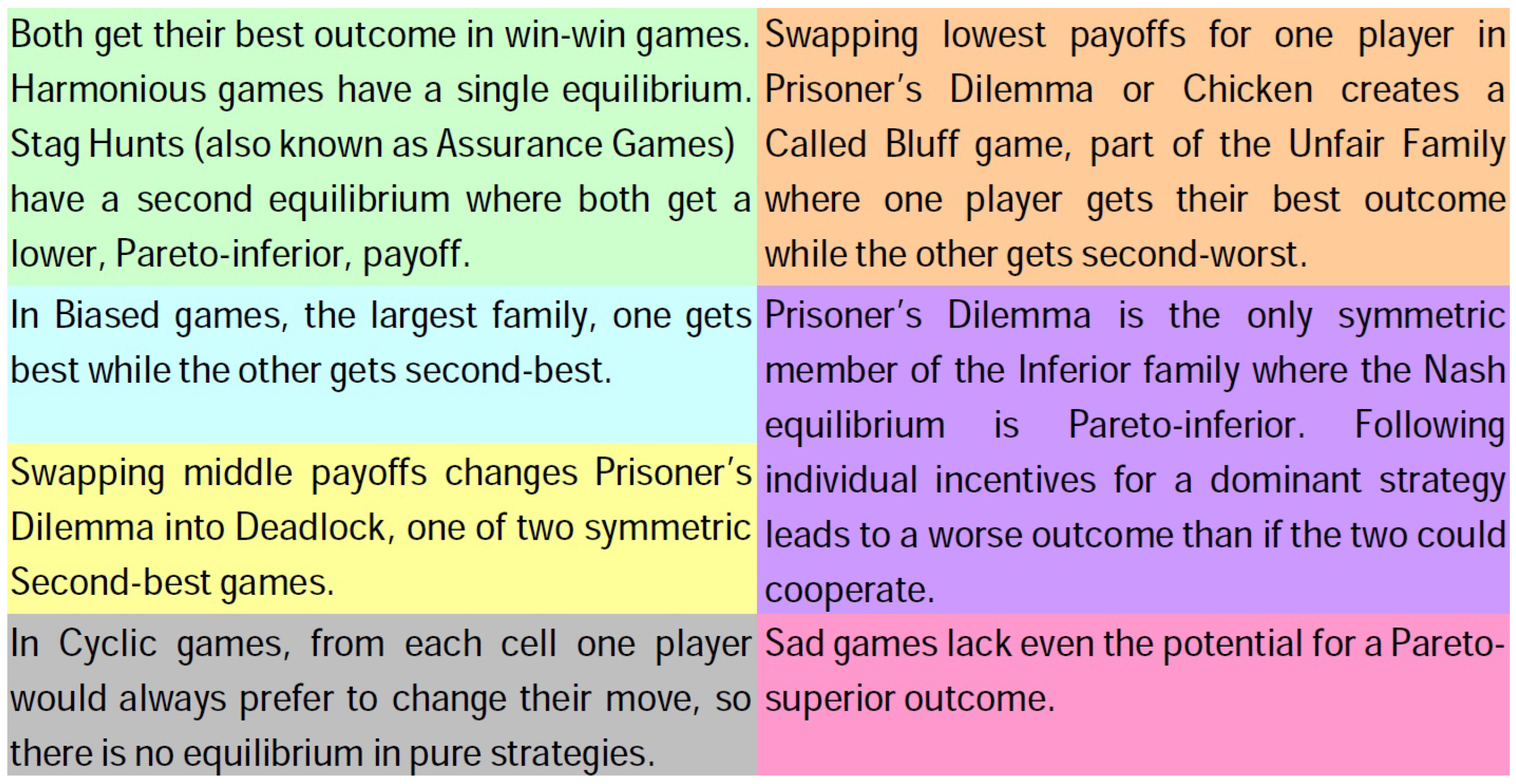
Figure 5 presents the $2\times 2$ games in a periodic table (Bruns, 2015a), which are organized around the symmetric $2\times 2$ games on a diagonal axis, highlighting the twelve strict ordinal games in which each DM has four distinct utilities. The patterns of utilities of the symmetric games combine to form asymmetric games, thus constituting a convenient basis for naming the games. The utilities in Nash equilibria classify the games into families, which are represented by colors according to Figure 6. It is worth noting here that the concept of cyclic games in Figure 5 is not the same as the analysis of cycles in $L_h$ stability, which is being investigated in this paper. Cyclical games refer to games that do not have Nash equilibrium in pure strategies, which simply means that they do not have any $L_1$ equilibrium, as Nash stability is equivalent to $L_1$ (Fang et al., 1993).

By relating the original table, Figure 5, to our results on cycles, Figure 4, we can draw some interesting conclusions. First, our method also classifies all games in seven categories. Then, we observe that all games that present a cycle of length 2, from the horizon equal to 2, belong to the group that does not have a Nash equilibrium in pure strategies (gray group in Figure 5). Furthermore, all games in which both DMs achieve the best result in the equilibrium (green group in Figure 5) present cycle 1, from the horizon equal to 3. Finally, all games classified as “sad”, that is, those that do not even have the potential for a Pareto-superior result (pink group in Figure 5), also have cycle 1, from the horizon equal to 2.

4.2. Classification of $2\times 2$ Games Through Response Graph-Based Workflow

Omidshafiei et al. (2020) proposed a methodology based on $\alpha$-Rank response graph and game theory to characterize the topological landscape of multiplayer games. These authors demonstrate how the topological structure over games can be used to automatically generate games with interesting characteristics for learning agents.

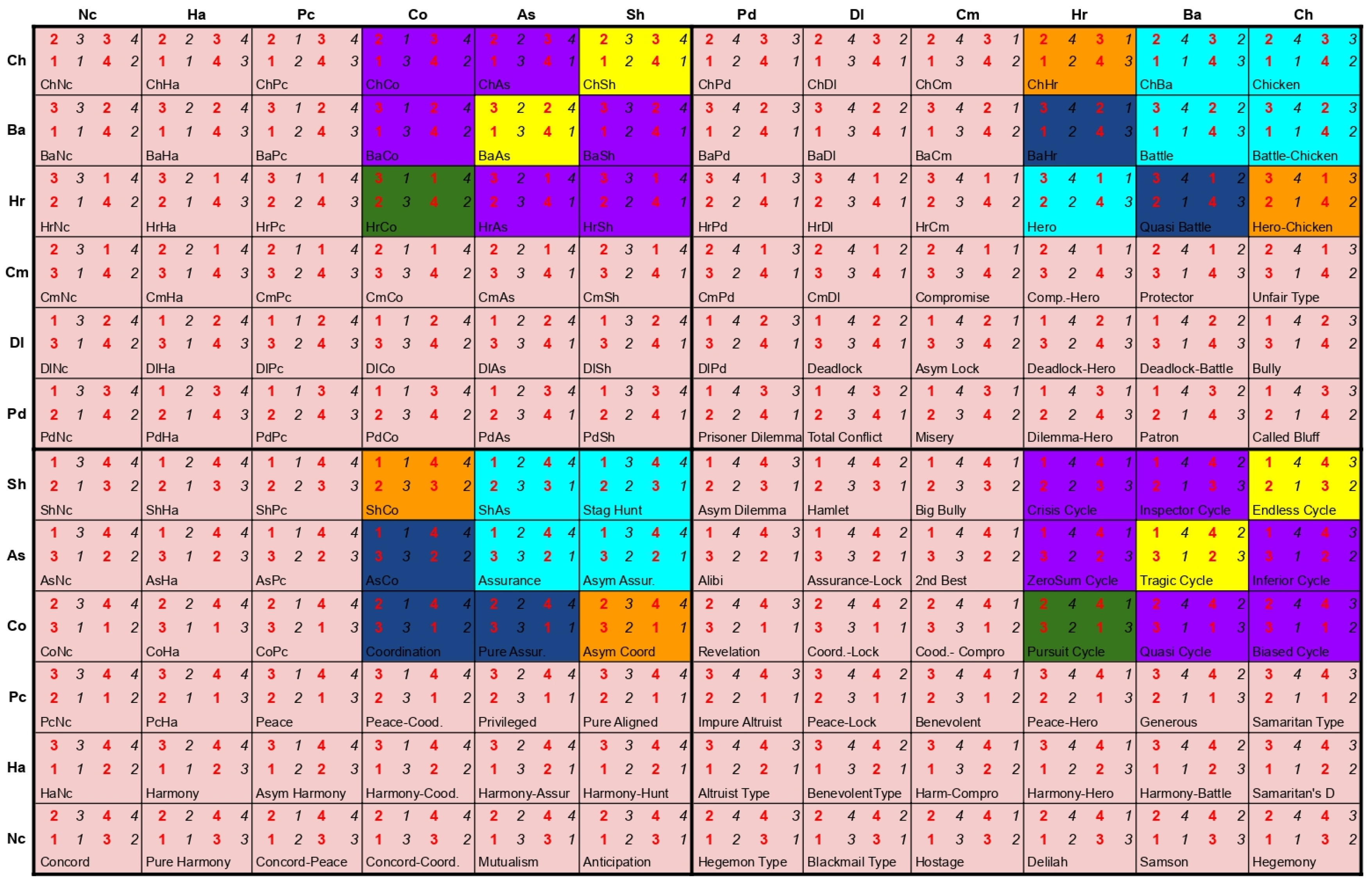
A discussion of the methodology used to classify $2\times 2$ games appears in the Supplementary Note 2 of the Supplementary Information of Omidshafiei et al. (2020). The vertices of the $\alpha$-Rank response graph consist of the four possible strategy profiles, and there is an edge between two strategy profiles if having a deviation from a single DM can switch between them. Associated with each edge is a transition probability that depends on the utilities of the deviating DM for both strategy profiles and on a parameter $\alpha$ that captures a notion of selection pressure. After computing $\alpha$-Rank response graphs, the authors symmetrize the graph, perform an spectral analysis, and collect graph measures. Finally, they ran a Principal Component Analysis on the collection of 144 games and grouped them into seven clusters based on their top 2 principal components. The results with $\alpha =0.2$ and $\alpha =0.01$ are reproduced in Figure 7 and Figure 8, respectively. As pointed out by Omidshafiei et al. (2020), the colors in these figures have no meaning; they are only used to distinguish the different group of games found by their method. An observation that can be made is that our classification, shown in Figure 4, is closer to the original classification of Bruns (2015a), shown in Figure 5, than both classifications provided in Omidshafiei et al. (2020).

Comparing the classification presented in Figure 7 with the grouping proposed in this work, shown in Figure 4, we observe that all games with a cycle length of 1, from $h=1$, and $h=6$, as well all games with a cycle length 4 from $h=2$ and $h=3$, belong to the group of games represented in light red in Figure 7. On the other hand, the games displayed in light blue, dark blue, and orange correspond to games with a cycle length of 1 from $h=3$, while the games in the green group are classified as games with a cycle length 2 from $h=2$.

By comparing the game grouping in Figure 8 with the classification proposed in Figure 4, we observe that all games with a cycle length 1, from $h=6$, and all games with a cycle length 4, from $h=3$, belong to the light red group in Figure 8. Likewise, all games with a cycle length 2 from $h=2$ are part of the yellow group in the same figure. Furthermore, the games represented in light blue, orange, and green in Figure 8 correspond to games with a cycle length 1 from $h=3$.

4.3. Harmony Index

In $2\times 2$ games, let us call the row DM as DM 0 and the column DM as DM 1. Let $u_i(s_m,s_n)$ be the utility for DM i when DM 0 chooses strategy $s_m$ and DM 1 chooses strategy $s_n$, for $i,m,n\in \{0,1\}$. The harmony index, as defined by Zizzo (2002), is given by the Pearson correlation of the utility vectors: $(u_0(s_0,s_0),u_0(s_0,s_1),u_0(s_1,s_0),u_0(s_1,s_1))$ and $\left((u_1(s_0,s_0),u_1(s_0,s_1),u_1(s_1,s_0),u_1(s_1,s_1))\right)$.1 Intuitively, the higher the harmony index is, the more in the same direction the utilities of the DMs are, increasing the likelihood of cooperative behavior in the game.

Figure 9 presents the harmony index values calculated for each $2\times 2$ game. Each index is shown in parentheses next to the corresponding game name. For example, ChNc ($0.4$) indicates that the harmony index for the ChNc game is $0.4$.

More specifically, note that the games with a cycle length of 2, from horizon $h=2$ onward (red group in Figure 9) and the games with a cycle length of 1, from horizon $h=5$ onward (intermediate gray group in Figure 9), all have harmony index values less than or equal to zero. In contrast, the games with a cycle length of 4, from horizon $h=3$ onward (dark blue group in Figure 9) and the games with a cycle length of 1, from horizon $h=6$ onward (dark gray group in Figure 9), and all games in the third quadrant (which are the win–win games) all show harmony indices greater than or equal to zero. In other words, these are games in which a positive correlation is observed between DMs’ utilities, which may lead to harmony or cooperative behavior.

In general, it can be observed that there is no well-defined relationship between the harmony index and the cycle length in $2\times 2$ games. In other words, there is no linear relationship between these variables, since, by analyzing Figure 9, it becomes clear that an increase in cycle length does not have a positive or negative trend in the harmony index.

4.4. Conflict Index

The idea of the conflict index proposed by Gimon and Leonetti (2025) is to calculate an average of the four normalized angles between the main diagonal and each line that connects the two pairs of utilities that correspond to two strategy profiles that differ in the strategy of only one DM. In this paper, we present an alternative way to obtain the same index values.

Formally, for any DM $i\in \{0,1\}$, assuming that the opponent, DM $1-i$, uses strategy $s_m$ for $m\in \{0,1\}$, we are interested in the following angle:

$${\alpha }_{i,m}=co{s}^{-1}\left({\displaystyle \frac{\overrightarrow{x}·{\overrightarrow{y}}_{i,m}}{\parallel \overrightarrow{x}\parallel \parallel {\overrightarrow{y}}_{i,m}\parallel }}\right),$$

where · represents the dot product of two vectors, $\parallel \overrightarrow{x}\parallel$ is the Euclidean norm of $\overrightarrow{x}$, $\overrightarrow{x}=(1,1)$, ${\overrightarrow{y}}_{0,m}=(u_0(s_1,s_m)-u_0(s_0,s_m),u_1(s_1,s_m)-u_1(s_0,s_m))$, and ${\overrightarrow{y}}_{1,m}=(u_0(s_m,s_1)-u_0(s_m,s_0),u_1(s_m,s_1)-u_1(s_m,s_0))$.

Since the conflict index should be invariant to role reversals between the DMs, the following normalization is used to measure how distant from orthogonality is each one of the four lines from the main diagonal:

$${\alpha }_{i,m}^{\prime }={\displaystyle \frac{\pi }{2}}-\left|\left|{\alpha }_{i,m}-{\displaystyle \frac{\pi }{2}}\right|\right|.$$

Finally, to obtain a single index between 0 and 1, the following normalized version is proposed for the conflict index:

$$CI=\left({\displaystyle \frac{2}{\pi }}\right)\left({\displaystyle \frac{1}{4}}\right)\left(\sum _{i=0}^1\sum _{m=0}^1{\alpha }_{i,m}^{\prime }\right).$$

Intuitively, the higher the conflict index is, the more the increase of utility of one DM implies decrease in the utility of the other DM. Thus, a higher conflict index increases the likelihood of non-cooperative behavior.

Figure 10 presents the conflict index values calculated for each one of the $2\times 2$ games. Each index is shown in parentheses next to the corresponding game name. For example, PdNc ($0.5$) indicates that the conflict index for the PdNc game is 0.5. We note that all games with cycle length 2 from horizon 2, displayed in red in Figure 10, have a conflict index greater than or equal to 0.64, indicating a non-cooperative situation for these games. Almost all games with cycle length 1 from horizon 2, with the unique exception of games ChCm and Cmch, have conflict indices greater than or equal to 0.5, also indicating a non-cooperative trend of these games.

5. Conclusions

In this work, we explore cycles in $L_h$ stability. We illustrate this cyclic analysis using the periodic table for $2\times 2$ games, as presented by Bruns (2015a). In this analysis, we were able to confirm, in $2\times 2$ games, a conjecture made by Fang et al. (1993) that all $L_h$ cycles have length 1, 2, or 4. We do not address them here, but similar questions arise regarding the more recent stability definitions that also depend on horizon, such as $maximi{n}_h$ (Rêgo & Vieira, 2019), credible maximin (Rêgo et al., 2023), optimism–pessimism stability (Sabino & Rêgo, 2023, 2025), and minimax regret stability (Sabino & Rêgo, 2024). Whether the conjecture made by Fang et al. (1993) is valid for a more general class of games remains an open question.

Our study generates a new classification of $2\times 2$ games according to the length of the cycle and to the horizon in which the cycles begin. Finally, we relate our classification with those of Bruns (2015a) and of Omidshafiei et al. (2020). Finally, we also investigate how harmony and conflict indices vary across our classes of games.

References

1. Brams, S. (1977). Deception in 2 × 2 games. Journal of Peace Science, 2, 171–203. [Google Scholar] [CrossRef]
2. Brams, S., & Kilgour, D. (2009). How democracy resolves conflict in difficult games. In S. Levin (Ed.), Games, groups, and the global good (pp. 229–241). Springer. [Google Scholar]
3. Bruns, B. (2015a). Atlas of 2 × 2 games: Transforming conflict and cooperation (Working paper). Vincent and Elinor Ostrom Workshop in Political Theory and Policy Analysis. [Google Scholar]
4. Bruns, B. (2015b). Names for games: Locating 2 × 2 games. Games, 6(4), 495–520. [Google Scholar] [CrossRef]
5. Fang, L., Hipel, K. W., & Kilgour, D. M. (1993). Interactive decision making: The graph model for conflict resolution (Vol. 3). John Wiley & Sons. [Google Scholar]
6. Fishburn, P., & Kilgour, D. (1990). Binary 2 × 2 games. Theory and Decision, 29(3), 165–182. [Google Scholar] [CrossRef]
7. Fraser, N. M., & Hipel, K. W. (1984). Conflict analysis: Models and resolutions (Vol. 11). North-Holland. [Google Scholar]
8. Fraser, N. M., & Kilgour, D. M. (1986). Non-strict ordinal 2 × 2 games: A comprehensive computer-assisted analysis of the 726 possibilities. Theory and Decision, 20(2), 99–121. [Google Scholar] [CrossRef]
9. Gimon, D., & Leonetti, A. B. (2025). On quantifying the conflict in 2 × 2 games. In M. T. Escobar, A. Turón, G. Ke, & J. Aguarón (Eds.), Proceedings of the 25th international conference on group decision and negotiation, Zaragoza, Spain, June 15–18 (pp. 21–29). INFORMS GDN. [Google Scholar]
10. Howard, N. (1971). Paradoxes of rationality: Games, metagames, and political behavior. MIT Press. [Google Scholar]
11. Kilgour, D. M. (1985). Anticipation and stability in two-person noncooperative games. Dynamic Models of International Conflict, 26–51. [Google Scholar] [CrossRef]
12. Kilgour, D. M., & Fraser, N. M. (1988). A taxonomy of all ordinal 2 × 2 games. Theory and Decision, 24(2), 99–117. [Google Scholar] [CrossRef]
13. Kilgour, D. M., Hipel, K. W., & Fang, L. (1987). The graph model for conflicts. Automatica, 23(1), 41–55. [Google Scholar] [CrossRef]
14. Nash, J. F. (1950). Equilibrium points in n-person games. Proceedings of the National Academy of Sciences of the United States of America, 36(1), 48–49. [Google Scholar] [CrossRef] [PubMed]
15. Omidshafiei, S., Tuyls, K., Czarnecki, W. M., Santos, F. C., Rowland, M., Connor, J., Hennes, D., Muller, P., Perolat, J., Vylder, B. D., Gruslys, A., & Munos, R. (2020). Navigating the landscape of multiplayer games. Nature Communications, 11, 5603. [Google Scholar] [CrossRef] [PubMed]
16. Rapoport, A., & Guyer, M. (1966). A taxonomy of 2 × 2 games. General Systems, 11, 203–214. [Google Scholar]
17. Rapoport, A., Guyer, M. J., & Gordon, D. G. (1976). The 2 × 2 game. University of Michigan Press. [Google Scholar]
18. Rêgo, L. C., & Vieira, G. I. A. (2017). Symmetric sequential stability in the graph model for conflict resolution with multiple decision makers. Group Decision and Negotiation, 26, 775–792. [Google Scholar] [CrossRef]
19. Rêgo, L. C., & Vieira, G. I. A. (2019). Maximinh stability in the graph model for conflict resolution for bilateral conflicts. IEEE Transactions on Systems, Man, and Cybernetics: Systems, 50(10), 3760–3769. [Google Scholar] [CrossRef]
20. Rêgo, L. C., Vieira, G. I. A., & Kilgour, D. M. (2023). The graph model for conflict resolution and credible maximin stability. IEEE Transactions on Systems, Man, and Cybernetics: Systems, 53(2), 947–956. [Google Scholar] [CrossRef]
21. Robinson, D., & Goforth, D. (2004). Topology of 2 × 2 games (1st ed.). Routledge. [Google Scholar] [CrossRef]
22. Sabino, E. R., & Rêgo, L. C. (2023). Optimism pessimism stability in the graph model for conflict resolution for multilateral conflicts. European Journal of Operational Research, 309(2), 671–682. [Google Scholar] [CrossRef]
23. Sabino, E. R., & Rêgo, L. C. (2024). Minimax regret stability in the graph model for conflict resolution. European Journal of Operational Research, 314(3), 1087–1097. [Google Scholar] [CrossRef]
24. Sabino, E. R., & Rêgo, L. C. (2025). Introducing Credible Movements in the Optimism Pessimism Stability in the Graph Model. Group Decision and Negotiation, 34(1), 177–207. [Google Scholar] [CrossRef]
25. Zagare, F. (1984). Limited-move equilibria In 2 × 2 games. Theory and Decision, 16, 1–19. [Google Scholar] [CrossRef]
26. Zizzo, D. J. (2002). On the measurement of harmony in normal form games (Economics series working papers No. 116). University of Oxford, Department of Economics. Available online: https://ideas.repec.org/p/oxf/wpaper/116.html (accessed on 9 September 2025).
Figure 2. BaCo game graph model.
Games 16 00054 g002
Figure 3. Game tree of horizon 5 from state s 1 with initial move from DM i.
Games 16 00054 g003
Figure 4. Diagram of the topology of games 2 × 2 by L h cycles and horizons.
Games 16 00054 g004
Figure 5. 2 × 2 Game topology diagram. Adapted from (Bruns, 2015a).
Games 16 00054 g005
Figure 6. Color legend for game table 2 × 2 . Adapted from (Bruns, 2015a).
Games 16 00054 g006
Figure 7. Clusters of 2 × 2 games based on high α -Rank, for α = 0.2 . Source: Adapted from Supplementary Material of Omidshafiei et al. (2020).
Games 16 00054 g007
Figure 8. Clusters of 2 × 2 games based on low α -Rank, for α = 0.01 . Source: Adapted from Supplementary Material of Omidshafiei et al. (2020).
Games 16 00054 g008
Figure 9. Harmony index for all 2 × 2 strictly ordinal games.
Games 16 00054 g009
Figure 10. Conflict index for all 2 × 2 strictly ordinal games.
Games 16 00054 g010