

“Anything Goes” in an Ultimatum Game?


Department of Political Economy & Moral Science, University of Arizona, Social Sciences 213, 1145 E. South Campus Drive, Tucson, AZ 85721, USA
Games 2025, 16(4), 36; https://doi.org/10.3390/g16040036
Submission received: 8 June 2024
/
Revised: 4 June 2025
/
Accepted: 4 July 2025
/
Published: 9 July 2025
(This article belongs to the Special Issue Evolution of Cooperation and Evolutionary Game Theory)
Abstract
I consider an underexplored possible explainer of the “surprising” results of Ultimatum Game experiments, namely, that Proposers and Recipients consider following only some of all the logically possible strategies of their Ultimatum Game. I present an evolutionary analysis of different games having the same set of allowable Proposer offers and functions that determine Proposer and Recipient payoffs. For Unrestricted Ultimatum Games, where Recipients may choose from among any of the logically possible pure strategies, populations tend to evolve most often to Nash equilibria where Proposers make the lowest allowable offer. However, for Threshold Reduced Ultimatum Games, where Recipients must choose from among minimum acceptable offer strategies, and for Range Reduced Ultimatum Games, where Recipients must choose from among pure strategies that spurn offers that are “too high” as well as “too low”, populations tend to evolve most often to Nash equilibria where Proposers offer substantially more than the lowest possible offer, a result that is consistent with existing Ultimatum Game experimental results. Finally, I argue that, practically speaking, actual Proposers and Recipients will likely regard some reduction of the Unrestricted Ultimatum Game as their game because, for them, the strategies of this reduction are salient.
1. Introduction
The Ultimatum Game is one of the simplest of asynchronous division games. Two agents, a Proposer and a Recipient, have an opportunity to divide some fixed quantity of a good, such as a cake or a sum of money. The Proposer offers the Recipient some fraction x of M. Then the Recipient either accepts or spurns the Proposer’s offer. If the Recipient accepts, the Recipient receives the offered x-share and the Proposer keeps the remaining -share. If the Recipient spurns, both get nothing. Ultimatum Games and their variants have been mainstays of experimental economics ever since Werner Güth, Rolf Schmittberger, and Bernd Schwarze published the first Ultimatum Game experimental study in 1982 (Güth et al., 1982). In their original study, forty-two subjects engaged in two rounds of twenty-one Ultimatum Games, where M was 4–10 German marks. In the first round, the average Proposer offer was just over , only two Recipients spurned, and one of these Recipients spurned an offer of more than 1 mark. In the second round, the average Proposer offer was , six Recipients spurned and five of these Recipients spurned offers of at least 1 mark.1 In Behavioral Game Theory, Colin Camerer wryly remarks, “In 1982, Güth, Schmittberger and Schwarze reported the kind of empirical finding that surprises only economists” (Camerer, 2003, p. 43).
Ultimatum Games generate great interest because the standard backwards induction analysis of these games is so simple, yet actual individuals who engage in these games so systematically fail to follow the outcomes predicted by this analysis. According to this well-known analysis, the Proposer should offer the lowest possible positive x-share, which the Recipient should then accept. Starting with the original study of Güth et al. (1982), subjects in Ultimatum Game experiments tend not to follow the outcomes they “should” follow according to this analysis. Camerer (2003, pp. 48–83) and Güth and Kocher (2014) summarize the best-known results of Ultimatum Game experiments. Phenomena consistent with the original results of Güth et al. (1982) have been confirmed in many experiments performed in different cultures having high degrees of cooperative activity and of market integration.2 In these cultures, modal and median Proposer offers are usually – and mean offers are –. Proposers seldom make especially low offers of – or hyperfair offers of more than . Recipients seldom spurn offers of – and spurn offers of less than about half the time. Experimental subjects of some cultures with lower degrees of cooperative activity and of market integration behave somewhat differently. In some experiments in these cultures, the modal and mean Proposer offers are much lower than those of the more cooperative and market-integrated cultures and Recipients hardly ever spurn offers. Additionally, in some of these cultures, Proposers sometimes do offer more than and Recipients tend to reject these hyperfair offers!
What explains all this “surprising” behavior in Ultimatum Games? The ongoing research program motivated by this question has two main areas that overlap considerably. Researchers working in the first main area propose and test with experiments with different models of how real individuals perceive and evaluate their options in an Ultimatum Game. Researchers working in the second main area analyze evolutionary models of behavioral patterns that might evolve among the members of a population who engage in Ultimatum Games repeatedly over time. In my opinion, the existing research focuses on questioning underlying assumptions of the standard backwards induction analysis regarding what motivates agents’ choices and how agents choose. This analysis assumes that the agents who engage in an Ultimatum Game are Bayesian rational, so that each consistently chooses so as to maximize her expected payoff, and nontuistic, so that the payoff of each depends solely upon her own endowment of goods, and not upon the endowments of others. Some directly challenge the idea that real individuals are nontuistic. For example, Fehr and Schmidt (1999) and Bicchieri (2005, pp. 100–139) propose utility functions where a Recipient’s payoff can depend in part upon what the Proposer receives and what he receives. Others challenge the idea that real individuals always choose as Bayesian rational agents choose. For example, Gale et al. (1995), Skyrms (2014), and Harms (1997) propose evolutionary models where those in the roles of Proposer and Recipient do not always follow options that maximize expected payoff. Overall, this existing research tries to explain “surprising” behavior in Ultimatum Games by exploring how actual individuals might differ from the homo economicus of some economics textbooks.
In this paper, I consider another and an underexplored possible explainer of these “surprising” results, namely, that the agents consider following only some of all the logically possible strategies of their Ultimatum Game. Such agents effectively engage in a reduction of their Ultimatum Game. The Ultimatum Game of the standard backwards induction analysis is a game of perfect information, where the Recipient first observes the Proposer’s offer and then chooses either to accept or to spurn. In this “ordinary” Ultimatum Game, the Recipient’s choice given a particular offer does not depend upon what he would have chosen at any of the other offers. The Recipient can follow any of the logically possible pure strategy responses to the set of Proposer offers. In this “ordinary” or Unrestricted Ultimatum Game (hereafter Unrestricted UG), “anything goes” for the Recipient in terms of allowable strategies, which is why I use the adjective “unrestricted” for emphasis. In this paper, I will propose that, for many games having an Ultimatum Game-like structure where the Recipient either accepts or spurns the Proposer’s offer, the Proposer and Recipient will regard only some special subset of all the logically possible strategies in the corresponding Unrestricted UG as live options for them. This is because, in these games, the set of Recipient pure strategies in the corresponding Unrestricted UG will be so large, and many of the constituent Recipient pure strategies so complex, that actual Proposers and actual Recipients will focus their attention exclusively upon some subset of the logically possible Recipient pure strategies, and the pure strategy profiles containing them, that they regard as “natural” or salient for them. Such agents effectively engage in a reduced Ultimatum Game where they follow their ends of one of these salient strategy profiles.
In fact, many existing Ultimatum Games studies are based upon a particular reduced Ultimatum Game. In these studies, the Recipients are either instructed to focus upon or allowed to follow only threshold strategies. A threshold strategy, also known as a monotone or minimum acceptable offer strategy, is such that a Recipient accepts all and only offers equal to or greater than some threshold share. The resulting game is a Threshold Reduced Ultimatum Game (hereafter Threshold RUG). In some experiments, Recipients are asked to give their responses in terms of threshold strategies.3 Nearly all evolutionary studies of the Ultimatum Game limit the Recipient pure strategies to threshold strategies.4 A Threshold RUG is vastly simpler, and consequently easier to analyze, than its counterpart Unrestricted UG. However, I will argue below that, from a rational choice perspective, there is no good reason to regard any particular subset of Recipient strategies, including the threshold strategies, as a priori privileged.
How do restrictions on the pure strategies the Recipients may follow affect the outcomes of an Ultimatum Game? This question has not been addressed systematically in previous Ultimatum Game studies. In particular, to date, there have been no experimental studies that compare how Proposers and Recipients tend to choose in Unrestricted UGs and in Threshold RUGs. Likewise, there have been no evolutionary studies that compare evolutionary processes applied to both Unrestricted UGs and Threshold RUGs. In this paper, I present an evolutionary analysis of sets of Ultimatum Games where the Proposer’s allowable offers are held fixed and the Recipient’s set of pure strategy responses can vary. More specifically, in a given set of these n-piece Ultimatum Games, the Proposer may make one of n distinct offers and each resulting game in the set is characterized by one of the following Recipient strategy sets:
- (U.1)
- All logically possible pure strategies (“anything goes”), so that the game is an n-piece Unrestricted UG;
- (U.2)
- Threshold strategies, so that the game is an n-piece Threshold RUG;
- (U.3)
- Singleton strategies where the Recipient accepts only exact offers, so that the game is an n-piece Singleton Restricted Ultimatum Game (hereafter Singleton RUG), and
- (U.4)
- Range strategies where the Recipient accepts only offers lying within a given “connected” range, so that the game is an n-piece Range Restricted Ultimatum Game (hereafter Range RUG).
I apply a 2-population replicator dynamic model of evolution to the games in these sets and show by example that populations whose members’ behavior evolves according to this model tend to reach quite different outcome distributions depending upon which pure strategies Recipients may follow. In n-piece unrestricted UGs, populations tend to evolve most often to Nash equilibria where the Proposer is “most greedy” and makes the lowest possible offer. However in n-piece Threshold RUGs, Singleton RUGs, and Range RUGs, populations tend to evolve most often to Nash equilibria where the Proposer offers substantially more than the lowest possible offer. Therefore, for an evolving Recipient population, “less can be more”, in the sense that Recipient populations whose pure strategies are restricted in certain ways can more often reach equilibria more favorable to them than a lowest possible offer equilibrium than can Recipient populations where “anything goes”.
The remainder of the paper is structured as follows: In Section 2, I discuss some related evolutionary studies of Ultimatum Games. Most of these earlier studies focus upon Threshold RUGs, and none try to compare the evolution of behavior in Threshold UGs and in Unrestricted UGs, as is done in this paper. In Section 3, I argue that, a given set of Proposer offers and a pair of payoff functions characterize an entire family of games. Members of this family include an Unrestricted UG and games with various restrictions on Recipient strategy sets such as a Threshold RUG, a Singleton RUG, and a Range RUG. I refer to all of the games in such a given family as Ultimatum Games, although admittedly, only the Unrestricted UG is a “true” Ultimatum Game by definition. In Section 4, I apply a 2-population replicator dynamic model to each of the four games (U.1), (U.2), (U.3), and (U.4) for and . Here, I give the results of a series of simulations of replicator dynamic evolution applied to these games. In Section 5, I first discuss in more detail how the Section 4 simulation results are related to the results of previous evolutionary Ultimatum Game studies. I next discuss how the Section 4 results support my claims above that populations that engage in an n-piece Unrestricted UG evolve most often to Nash equilibria most favorable to the Proposer, while populations that engage in an n-piece Threshold RUG, Singleton RUG, or Range RUG evolve most often to Nash equilibria that are better for the Recipient than equilibria most favorable to the Proposer. Interestingly, for the n-piece Unrestricted UG, while the limits of replicator dynamic evolution are most often Nash equilibria where the Proposer makes the smallest possible offer, most of these equilibria are not subgame perfect. Replicator dynamic simulation results for the n-piece Threshold RUG are consistent with the results of earlier evolutionary studies of Threshold RUGs and also are broadly consistent with well-known results of Ultimatum Game experiments such as those discussed above. However, this does not amount to a vindication of the emphasis on or limitation to threshold strategies in many existing Ultimatum Game studies. This is because one obtains simulation results for the n-piece Range RUG similar to those of the n-piece Threshold RUG. Therefore, it is not so clear that evolutionary analyses should focus on Threshold RUGs, after all. Finally, in the closing Section 6, I argue that the Section 3 examples suggest that the Ultimatum Games of a given set of Proposer offers lie along a continuum of strategy sets. I argue that, from a purely rational choice perspective, the “right” Ultimatum Game is the Unrestricted UG, where “anything goes” for Recipient pure strategies. However, I also argue that, from a practical standpoint, in most cases, actual Proposers and Recipients will likely regard some reduced Ultimatum Game as their game. Here, I discuss in more detail why I believe that strategy salience is important in understanding how actual Proposers and Recipients understand and engage in an Ultimatum Game and merits further investigation.
2. Related Evolutionary Ultimatum Game Studies
The evolutionary analyses of n-piece Ultimatum Games given below complement the previous studies of Skyrms (2014), Harms (1997), Roth and Erev (1995), and Gale et al. (1995). These earlier studies explore how behavior might evolve in a Threshold RUG or an Unrestricted UG without trying to compare the evolutions of behaviors in several different types of n-piece Ultimatum Games as is done in this paper. All of these studies incorporate the results of computer simulations of evolutionary dynamics, as is done in this paper. In most of these earlier studies, as in this paper, the n-piece Ultimatum games analyzed have so many pure strategy profiles that the properties of the evolutionary dynamics applied to these games can only be explored computationally. Skyrms (2014) and Harms (1997) apply a 1-population replicator dynamic to n-piece Ultimatum Games where the members of a single population alternate between the roles of Proposer and Recipient and must adopt an overall strategy specifying which offer to make in the Proposer role and which offers to accept in the Recipient role. Unlike most authors who apply evolutionary dynamics to Ultimatum Games, Skyrms (2014) and Harms (1997) analyze some Unrestricted Ultimatum Games. Skyrms (2014) analyzes an Ultimatum Minigame, where one in the Proposer role can offer either a -share or an x-share for and in the Recipient role can follow any of the 4 logically possible pure strategy responses to the possible offers. Harms (1997) analyzes a similar Ultimatum Minigame and some 5-piece Ultimatum Games where one in the Recipient role can follow any of the 32 logically possible pure strategy responses to the possible offers. In the final section of his essay, Harms (1997) applies a 1-population replicator dynamic to a 12-piece Ultimatum Game where, in this case, he limits the Recipient pure strategies to the threshold strategies. Skyrms (2014) and Harms (1997) explore how certain weakly dominated strategies in the Ultimatum Games they analyze can persist in a population that evolves according to a 1-population replicator dynamic.
Roth and Erev (1995) and Gale et al. (1995) analyze n-piece Threshold RUGs using 2-population dynamical models. Roth and Erev (1995) and Gale et al. (1995) explore how evolutionary forces might produce behavioral patterns in two Proposer and Recipient populations similar to the “surprising” patterns observed in Ultimatum Game laboratory experiments. Roth and Erev (1995) apply a reinforcement learning model to a 9-piece Threshold RUG that has 9 Nash equilibria in pure strategies, including a subgame perfect equilibrium.5 Roth and Erev (1995) find that, in their simulations, when the orbits of reinforcement equilibrium converge, they tend to converge to Nash equilibria more favorable to the Recipient than the subgame perfect equilibrium. Gale et al. (1995) apply 2-population replicator dynamic models to a 40-piece Threshold RUG that has 40 Nash equilibria in pure strategies, including a subgame perfect equilibrium. In several sets of replicator dynamic simulations, they find that the populations converge most frequently to a Nash equilibrium substantially more favorable to the Recipient than the subgame perfect equilibrium.
3. Ultimatum Game Families
An Ultimatum Game, either unrestricted or reduced, is characterized by a set , a class of subsets of Z, and a pair of functions and that are strictly increasing over and where .6 Each Proposer pure strategy is an element , that is,
Each recipient pure strategy is a function of the form
So Z, the set of allowable offers, characterizes the Proposer’s pure strategies, and , the class of acceptance sets, characterizes the Recipient’s pure strategies. For a Proposer’s pure strategy, I use the admittedly clumsy identity function notation to emphasize that the pure strategies of both the Proposer and the Recipient are characterized by subsets of Z, although, for the Proposer, these subsets are always singletons. For a given pure strategy profile , the Recipient’s and Proposer’s respective payoff functions and are defined by
and
where is the indicator function of the set E.7 Therefore, the Recipient’s and the Proposer’s payoffs are determined entirely by , , and the acceptance sets of that “turn on” and when is in the acceptance set of a Recipient pure strategy and otherwise and otherwise “turn off” and . Below I will refer to and as the payoff determining functions. Throughout this paper, I will adopt the following common interpretation of this game: The Proposer and the Recipient have a chance to share a pie M, a fixed quantity of a homogeneous good. Any share of M is worth to the Proposer and to the Recipient. At a given strategy profile , with the Proposer offers an x-share of a pie to the Recipient, and with , the Recipient accepts (A) if and spurns (S) if . If the Recipient accepts , he receives the offered x-share, and the Proposer receives the remaining -share, and they achieve the payoff vector . If the Recipient spurns , they lose control over the disposition of the pie M, and both end up with a 0-share and achieve the payoff vector .
Can an acceptance set E be any subset of Z? If so, then “anything goes” for the Recipient; that is, the Recipient can follow any of the logically possible strategy responses to possible Proposer offers. In this case, the Proposer and Recipient are engaged in an Unrestricted UG where , the power class of Z. However, as noted in the Introduction, many Ultimatum Game studies restrict the Recipient pure strategies to the threshold strategies. Additionally, other limitations on the Recipient’s pure strategies in an Ultimatum Game are possible. In fact, I propose that a given Z of allowable Proposer offers together with a pair of payoff determining functions and characterize a whole family of games where the Proposer makes some offer that the Recipient then either accepts or spurns. A given member of this family is characterized by a particular class of acceptance sets. I will refer to such a family as a family of Ultimatum Games, though, in a sense, only the Unrestricted Ultimatum Game of this family is a “true” Ultimatum Game.
To illustrate the proposal just made, here, I give several examples of 5-piece Ultimatum Games, where, for each of these games, and . In these games, the pie is effectively divided into 6 equal-sized pieces of equal value to both the Proposer and the Recipient, and the Proposer must offer the Recipient at least 1 but no more than 5 pieces. Figure 1 summarizes an extensive form representation of the corresponding 5-piece Unrestricted UG. One might regard the Figure 1 game as simply the Ultimatum Game for this Z and payoff determining functions and , since, as in the general description of an Ultimatum Game in the Figure 1 game, the Proposer simply chooses for some , and then after observing , the Recipient then follows either A or S. The Figure 1 game is a game of perfect information with a unique subgame perfect equilibrium defined by the Proposer following the path and the Recipient following the paths A-if--if--if--if--if-. As the name suggests, in this 5-piece Unrestricted UG, “anything goes” for the Recipient, that is, , and the Recipient may follow any of the logically possible pure strategy responses to the Proposer’s possible offers. Figure 2 gives a strategic form representation of the Figure 1 game.
![Games 16 00036 g001]()
![Games 16 00036 g002]() In this game, is the Recipient strategy of accepting all offers, is the Recipient strategy of spurning all offers, and each of the other 30 pure Recipient strategies fall somewhere “in between” and in the sense that each requires the Recipient to accept some offers and to spurn others. For the Recipient, strictly dominates and weakly dominates the other 30 pure strategies. The Figure 2 game has 160 pure strategy profiles and 31 Nash equilibria in pure strategies, none of which are strict. One of these equilibria is , where the Proposer is “most greedy” and makes the lowest allowable offer and the Recipient is “most submissive” and accepts all offers. Every other pure strategy Nash equilibrium has the Recipient follow a pure strategy that requires him to spurn some positive offers. This game also has many partially mixed Nash equilibria where the Proposer offers and the Recipient follows a mixed strategy over all the pure strategies that accept . For example, if the Proposer follows , then, for every mixed strategy of the form
where is a probability distribution, and is a Nash equilibrium.8 These partially mixed Nash equilibria are members of Nash equilibrium components of this game. Nash equilibrium components of this and other Ultimatum Games will figure prominently in the evolutionary analysis in Section 4. is the unique Nash equilibrium where the Recipient is required to follow a best response to each possible offer, and characterizes the subgame perfect equilibrium of the Figure 1 game. Here and in the sequel, I will follow the lead of other Ultimatum Game studies and refer to any Nash equilibrium where the Recipient follows a best response to every Proposer offer as a subgame perfect equilibrium of the relevant Ultimatum Game, although, as I will explain shortly below, in some cases, I regard this a slight abuse of terminology. In the Figure 2 game, the subgame perfect equilibrium is one of 16 pure strategy Nash equilibria where the Recipient accepts the lowest offer . Therefore, if in fact the Proposer and the Recipient follow the paths and A-if- in the Figure 1 extensive form game, it is not a forgone conclusion that they are following their ends of the subgame perfect equilibrium of this game. The Recipient might be following one of the 15 pure strategies that accept other than the “most submissive” .
In this game, is the Recipient strategy of accepting all offers, is the Recipient strategy of spurning all offers, and each of the other 30 pure Recipient strategies fall somewhere “in between” and in the sense that each requires the Recipient to accept some offers and to spurn others. For the Recipient, strictly dominates and weakly dominates the other 30 pure strategies. The Figure 2 game has 160 pure strategy profiles and 31 Nash equilibria in pure strategies, none of which are strict. One of these equilibria is , where the Proposer is “most greedy” and makes the lowest allowable offer and the Recipient is “most submissive” and accepts all offers. Every other pure strategy Nash equilibrium has the Recipient follow a pure strategy that requires him to spurn some positive offers. This game also has many partially mixed Nash equilibria where the Proposer offers and the Recipient follows a mixed strategy over all the pure strategies that accept . For example, if the Proposer follows , then, for every mixed strategy of the form
where is a probability distribution, and is a Nash equilibrium.8 These partially mixed Nash equilibria are members of Nash equilibrium components of this game. Nash equilibrium components of this and other Ultimatum Games will figure prominently in the evolutionary analysis in Section 4. is the unique Nash equilibrium where the Recipient is required to follow a best response to each possible offer, and characterizes the subgame perfect equilibrium of the Figure 1 game. Here and in the sequel, I will follow the lead of other Ultimatum Game studies and refer to any Nash equilibrium where the Recipient follows a best response to every Proposer offer as a subgame perfect equilibrium of the relevant Ultimatum Game, although, as I will explain shortly below, in some cases, I regard this a slight abuse of terminology. In the Figure 2 game, the subgame perfect equilibrium is one of 16 pure strategy Nash equilibria where the Recipient accepts the lowest offer . Therefore, if in fact the Proposer and the Recipient follow the paths and A-if- in the Figure 1 extensive form game, it is not a forgone conclusion that they are following their ends of the subgame perfect equilibrium of this game. The Recipient might be following one of the 15 pure strategies that accept other than the “most submissive” .
Figure 1.
Five-piece unrestricted UG in extensive form.

Figure 2.
Five-piece unrestricted UG in strategic form (pure strategy Nash equilibria shaded).

Figure 3 summarizes the corresponding 5-piece Threshold RUG.
![Games 16 00036 g003]() As the name indicates, in the Figure 3 game, the Recipient’s pure strategies are the five threshold strategies only. In this game,
This game has 25 pure strategy profiles and 5 Nash equilibria in pure strategies, including the subgame perfect equilibrium that is also the unique strict Nash equilibrium. This game also has partially mixed Nash equilibria where the Proposer offers and the Recipient follows a mixed strategy over the pure strategies that accept . One can obtain the Figure 3 5-piece Threshold RUG by deleting in the Figure 2 game the 135 pure strategy profiles where the Recipient’s pure strategy is not a threshold strategy. However, unlike the Figure 2 game, the Figure 3 game is not derived from a game of perfect information. This game has no extensive form representation that is a game of perfect information, and in some of its extensive form representations, all of the Nash equilibria are subgame perfect. Figure 4 gives one such extensive form representation.
As the name indicates, in the Figure 3 game, the Recipient’s pure strategies are the five threshold strategies only. In this game,
This game has 25 pure strategy profiles and 5 Nash equilibria in pure strategies, including the subgame perfect equilibrium that is also the unique strict Nash equilibrium. This game also has partially mixed Nash equilibria where the Proposer offers and the Recipient follows a mixed strategy over the pure strategies that accept . One can obtain the Figure 3 5-piece Threshold RUG by deleting in the Figure 2 game the 135 pure strategy profiles where the Recipient’s pure strategy is not a threshold strategy. However, unlike the Figure 2 game, the Figure 3 game is not derived from a game of perfect information. This game has no extensive form representation that is a game of perfect information, and in some of its extensive form representations, all of the Nash equilibria are subgame perfect. Figure 4 gives one such extensive form representation.
![Games 16 00036 g004]() The Figure 4 game has no proper subgames, and so all of the Nash equilibria of this game are subgame perfect. So I think it is a slight abuse of terminology to refer to as the subgame perfect equilibrium of the Figure 3 game. However, since is the only Nash equilibrium that requires the Recipient to follow a best response to each Proposer offer, I think no confusion will arise by referring to as the subgame perfect equilibrium of the Figure 3 game and other 5-piece Ultimatum Games that contain this equilibrium.
The Figure 4 game has no proper subgames, and so all of the Nash equilibria of this game are subgame perfect. So I think it is a slight abuse of terminology to refer to as the subgame perfect equilibrium of the Figure 3 game. However, since is the only Nash equilibrium that requires the Recipient to follow a best response to each Proposer offer, I think no confusion will arise by referring to as the subgame perfect equilibrium of the Figure 3 game and other 5-piece Ultimatum Games that contain this equilibrium.
Figure 3.
Five-piece threshold RUG (pure strategy Nash equilibria shaded).
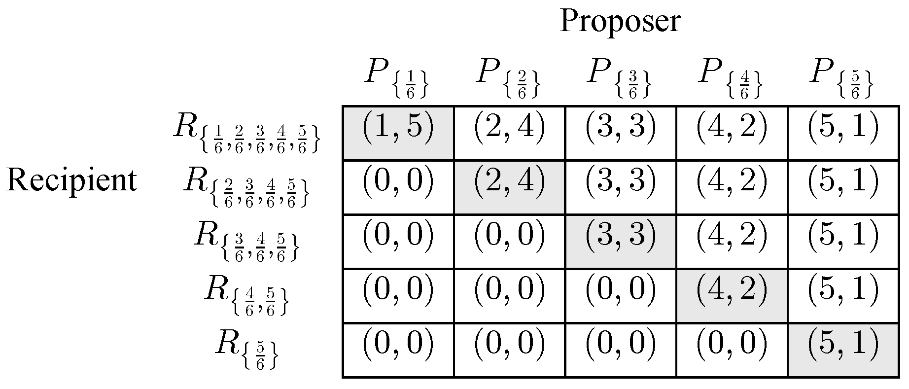
Figure 4.
Extensive form representation of Figure 3 game.
Figure 4.
Extensive form representation of Figure 3 game.
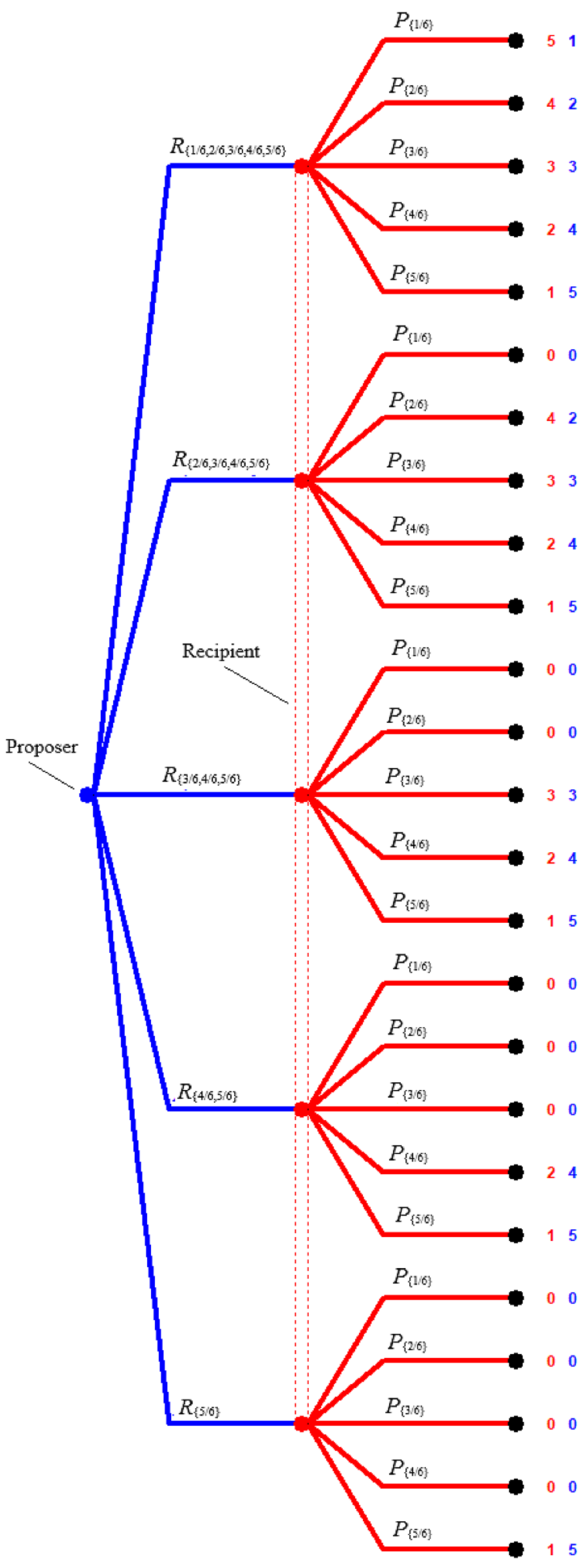
Figure 5 summarizes the corresponding 5-piece Singleton RUG.
In this game,
As the name of this game suggests, if the Recipient follows the singleton strategy for , then he accepts an offer of an -share of the pie M and no other offers. Informally, the Proposer has to get the offer “just right” in order to gain the Recipient’s acceptance. Since is not one of the Recipient’s acceptance sets in this game, the subgame perfect equilibrium of the Figure 2 and Figure 3 games is not present in the Figure 5 game. This game has 25 pure strategy profiles, 5 pure strategy Nash equilibria, and 26 mixed or partially mixed Nash equilibria. Unlike in the Figure 2 and Figure 3 games, in this game, all of the pure strategy Nash equilibria are strict. The Figure 5 game is an impure coordination game, sometimes called a discrete contract game (Young, 1998, p. 132), where the two engaging agents have available to them several strict Nash coordination equilibria over which their preferences conflict.
Figure 6 summarizes one more example of a member of this family of 5-piece Ultimatum Games.
![Games 16 00036 g006]() In this 5-piece Range RUG, the class of acceptance sets is
Each of the 15 acceptance sets of the Figure 6 game is “connected” in the sense that each defines a “range” over the ordered 6-tuple . More precisely, each acceptance set in is of the form for . The of the Figure 6 game includes the acceptance sets of the threshold strategies and the singleton strategies. Therefore, the Recipient can spurn offers that are “too low” or not exactly “on target”. This also includes some acceptance sets where the Recipient spurns offers that are “too high” and acceptance sets where the Recipient spurns offers that are either “too low” or “too high”. One obtains the Figure 6 game by deleting from the Figure 2 game the 85 strategy profiles where the Recipient follows a strategy , where the acceptance set E is “disconnected” in the sense that the Recipient accepts each of a pair of “endpoint” offers and but spurns some offers in between the acceptable “endpoint” offers. The Figure 6 game has 75 pure strategy profiles and 15 pure strategy Nash equilibria, including the subgame perfect equilibrium . None of these pure strategy Nash equilibria are strict. This game also has partially mixed Nash equilibria where the Proposer offers and the Recipient follows a mixed strategy over the pure strategies that accept .
In this 5-piece Range RUG, the class of acceptance sets is
Each of the 15 acceptance sets of the Figure 6 game is “connected” in the sense that each defines a “range” over the ordered 6-tuple . More precisely, each acceptance set in is of the form for . The of the Figure 6 game includes the acceptance sets of the threshold strategies and the singleton strategies. Therefore, the Recipient can spurn offers that are “too low” or not exactly “on target”. This also includes some acceptance sets where the Recipient spurns offers that are “too high” and acceptance sets where the Recipient spurns offers that are either “too low” or “too high”. One obtains the Figure 6 game by deleting from the Figure 2 game the 85 strategy profiles where the Recipient follows a strategy , where the acceptance set E is “disconnected” in the sense that the Recipient accepts each of a pair of “endpoint” offers and but spurns some offers in between the acceptable “endpoint” offers. The Figure 6 game has 75 pure strategy profiles and 15 pure strategy Nash equilibria, including the subgame perfect equilibrium . None of these pure strategy Nash equilibria are strict. This game also has partially mixed Nash equilibria where the Proposer offers and the Recipient follows a mixed strategy over the pure strategies that accept .
Figure 6.
Five-piece range RUG (pure strategy Nash equilibria shaded).

4. Evolutionary Dynamics Applied to -Piece Ultimatum Games
4.1. Description of the Replicator Dynamic Model
To explore the evolution of strategies in Ultimatum Games, I applied a replicator dynamic model to several members of families of n-piece Ultimatum Games. The evolution of strategies is described in terms of population states. For the first population, the Proposers, a Proposer population state is a distribution , where is the proportion of Proposers that follow and offer i of n pieces.9 denotes the special case where, at time t, all Proposers follow the pure strategy , and is of the form , where the ith component is 1. denotes the set of all possible Proposer population states or Proposer strategy simplex. For the second population, the Recipients, a Recipient population state is a distribution , where are the pure strategies for a Recipient as defined by and are the proportion of Recipients that follow . denotes the special case where, at time , all Recipients follow the pure strategy , and is of the form , where the jth component is 1. denotes the set of all possible Recipient population states or Recipient strategy simplex. denotes the product simplex of Recipient and Proposer strategy profiles. If the population states can vary according to time, then and are respectively the Proposer population state at time t and the Recipient population state at time t, where is the proportion of Proposers that follow at t and is the proportion of Recipients that follow at t.
The distributions of the population states and are respectively equivalent to the distributions of the mixed Proposer strategy
and the mixed Recipient strategy
A distribution pair characterizes a Nash equilibrium when the corresponding mixed strategy profile is a Nash equilibrium. A closed and connected set characterizes a Nash equilibrium component when each characterizes a Nash equilibrium. For ease of expositions, I will use the Section 3 strategy notations and the distribution notations presented here somewhat interchangeably to refer to strategies, strategy profiles, and Nash equilibria.
The 2-population replicator dynamic model I apply to the n-piece Ultimatum Games is summarized as follows: and are respectively the Proposer population and Recipient population initial states. For the Proposer population, the orbit evolves as from the initial state according to the n equations, as follows:
where, at time t, is the average payoff for a Proposer following , is the overall average payoff for Proposers, and is the Proposer mutation rate. For the Recipient population, the orbit evolves as from the initial state according to the equations, as follows:
where, at time t, is the average payoff for a Recipient following , is the overall average payoff for Recipients, and is the Recipient mutation rate.10 The equations of (1) and (2) define the laws of motion for the -perturbed replicator dynamic applied to this Ultimatum Game. In the special case where , (1) and (2) reduce to
and
the laws of motion of the deterministic replicator dynamic are applied to this Ultimatum Game.
If the orbits and of the 2-population deterministic replicator dynamic are applied to an Ultimatum Game, each approaches a limit distribution, that is, as and as ; then defines a Nash equilibrium. Additionally, for sufficiently small and , where the ratio remains constant, if the orbits and of the -perturbed replicator dynamic approach the limits as and as , then as , where is a Nash equilibrium. Some single Nash equilibria and some Nash equilibrium components can be attracting sets of replicator dynamics. For a given Nash equilibrium , if a set of distributions exists such that, for each initial state pair , the replicator orbits and converge respectively to and , then is the basin of attraction of and denotes the size of the basin , that is, the fraction of that occupies. Similarly, for a given Nash equilibrium component , if a set of distributions exists such that, for each initial state pair , the replicator orbits and converge respectively to some , then is the basin of attraction of and denotes the size of .
One can interpret the replicator dynamic as a model of how population members learn by imitation to follow more successful strategies. According to this imitation learning interpretation, at a given time t, a fraction of each population updates their current strategies, and if these updaters observe others in their population following strategies that are achieving higher payoffs than the overall average payoff given the current population states, they change to one of these strategies. For the deterministic replicator dynamic with laws of motion defined by (3) and (4), at any given time t, all updating Proposer and Recipient population members apply the learning rule correctly. For the -perturbed replicator dynamic with laws of motion defined by (1) and (2), at any give time t, the fraction of the updating Proposers applies the learning rule correctly and the fraction of the updating Proposers mutates, and the fraction of the updating Recipients applies the learning rule correctly, and the fraction of the updating Recipients mutates. If a Proposer mutates, then she adopts any of the n alternative Proposer pure strategies with equal probability. If a Recipient mutates, then he adopts any of the alternative pure strategies determined by with equal probability. One can interpret a mutation as a Proposer or a Recipient “slipping” by misperceiving the game in which they engage. A Proposer or Recipient who “slips” this way misapplies the learning rule so that the strategy she follows might differ from the strategy she would follow by applying the learning rule correctly.
4.2. Description of the Computer Simulations
I ran a series of simulations of 2-population replicator dynamics on the members of two sets of four games of a family of n-piece Ultimatum games. I built the simulator programs and ran these simulations using MATLAB Version 24.2.11 Each of these two sets of four n-piece games included
- (U.1)
- The n-piece Unrestricted UG;
- (U.2)
- The n-piece Threshold RUG;
- (U.3)
- The n-piece Singleton RUG; and
- (U.4)
- The n-piece Range RUG.
The first set of four games is the 5-piece Ultimatum Games discussed in Section 3. The second set of four is 10-piece counterpart games of the section Section 3 games.
To each member of each set of n-piece games, I applied four instances of the 2-population replicator dynamic model, as follows:
- (i)
- The deterministic replicator dynamic;
- (ii)
- The -perturbed replicator dynamic;
- (iii)
- The -perturbed replicator dynamic; and
- (iv)
- The -perturbed replicator dynamic.
I applied the deterministic replicator in order to explore which sets of Nash equilibria of Ultimatum Games can be attracting sets of the replicator when all populations members apply the imitation learning rule correctly. I applied the 0.001, 0.01-perturbed replicator dynamic, where , in order to produce results that can be readily compared with those of Gale et al. (1995), whose most striking findings occur when the Recipient mutation rate is much higher that the Proposer mutation rate . I applied the 0.001, 0.001-perturbed and -perturbed replicator dynamics in order to explore the effects of mutation in the learning process when Proposers and Recipients mutate at the same rate.
I built the simulator of the system of differential equations defined by (1) and (2) using a MATLAB ordinary differential equation solver that approximates the path each equation traces from its initial condition with a Runge–Kutta method. For each n-piece Ultimatum Game discussed below, I ran four simulations, one for each of the four instances of the 2-population replicator dynamic listed above. Each simulation consisted of 10,000 orbit pairs of 5000 time cycles for each orbit pair. For each of the 10,000 orbit pairs of a given simulation, the initial points that were the initial Proposer and Recipient population states and were selected at random from the simplexes and . I chose the large number of time cycles for each orbit pair of a simulation to ensure that each convergent orbit had sufficient time to approach its final limit.12
In each of these simulations, all or nearly all of the 10,000 orbit pairs converged to the -level, that is, reached a final state where at least of the Proposer population and at least of the Recipient population were following their ends of a pair of limits that either were or approached a Nash equilibrium. More specifically, for each 0.99, 0.99-convergent orbit pair, at the end of the 5000 time cycles, at least of the Proposer population was following a distribution and at least of the Recipient population was following a distribution where either characterizes or approximates a Nash equilibrium of the particular n-piece Ultimatum Game. For the results discussed below, I count the corresponding orbit pair as having reached the Nash equilibrium limit when this orbit pair converged to at least the level. This will make the subsequent discussion of the specific simulations somewhat less cumbersome and should cause no confusion since the simulations are run on either the deterministic replicator or a -perturbed replicator, where both values are approaching 0, and as already noted, the limit as and is a Nash equilibrium.
Below I summarize the simulator results for the 5-piece and 10-piece Ultimatum Games. I give considerably more explanation of the 5-piece Ultimatum Game results than the 10-piece Ultimatum Game results since the reader may easily apply the discussion of the 5-piece Ultimatum Game results to the 10-piece Ultimatum Game results.
4.2.1. Five-Piece Ultimatum Games
As discussed in Section 3, for these games, and . Requiring the Proposer to offer a positive share of the pie ensures that if a corresponding 5-piece Ultimatum Game has a subgame perfect equilibrium, then this subgame perfect equilibrium is unique.
Table 1 summarizes the -convergence rates of the simulations run on the four 5-piece Ultimatum games. For example, for the Unrestricted 5-piece Ultimatum Game and the -perturbed replicator dynamic where , the convergence rate was since 9999 of the 10,000 orbit pairs of this simulation converged to the level. For this game and the deterministic replicator dynamic, the -perturbed replicator dynamic and the -perturbed replicator dynamic, the convergence rate was because, for these simulations, all 10,000 orbit pairs converged to the level.
In most of the simulations, the limits of a convergent orbit pair consisted of a distribution pair of the form , equivalent to a Proposer offering and a Recipient following some mixture over the pure Recipient strategies that accept . For this reason, the simulation results in the following figures and tables are given in terms of Proposer offers. Figure 7 summarizes the distributions of Proposer strategies at the final population states of the simulations run on the four 5-piece Ultimatum Games. Table 2 summarizes the accompanying sizes of the basins of attraction of single-point Nash equilibria or Nash equilibrium components of these simulations.
One overall finding for the unrestricted 5-piece Ultimatum Game is that the populations converged most frequently to equilibria where Proposers are “most greedy” and offer the lowest allowable -share, but in general, these equilibria were not subgame perfect. For the deterministic replicator dynamic applied to this game, over the 10,000 orbit pairs, the modal offer was , with 6298 of the orbit pairs converging to a Nash equilibrium of the form , where the Proposer orbit converged to the state that defines the pure strategy and the Recipient orbit converged to some state equivalent to some mixture over the 16 pure Recipient strategies that accept . If denotes the set of the distributions equivalent to these mixtures, then together with forms a Nash equilibrium component
From the simulation results, the basin of attraction of this Nash equilibrium component has the size . This 5-piece Unrestricted UG has three more Nash equilibrium components structurally similar to that have non-negligible basins of attraction of the deterministic replicator dynamic: , where Proposers offer and , , where Proposers offer and and , where Proposers offer and . Therefore, when applied to the Unrestricted 5-piece Ultimatum Game, the deterministic replicator dynamic converged most often, and indeed in a substantial majority of the time, to some Nash equilibrium, where Proposers are “most greedy” and offer only . However, any one of these attracting Nash equilibria was generally not the subgame perfect equilibrium, because the Recipients’ pure strategies were some distribution in over the 16 pure strategies that accept rather than being concentrated on the distribution of the “most submissive” .
When the -perturbed replicator dynamics with and were applied to the unrestricted 5-piece Ultimatum Game, in each case, the populations again converged most often to a Nash equilibrium, where Proposers offer and Recipients accept this offer. For the -perturbed replicator dynamic, 6712 of the orbit pairs converged to a single partially mixed Nash equilibrium . The distribution
puts positive weight on all 16 pure Recipient strategies, where Recipients accept a offer, the highest being and the lowest being . The Nash equilibrium has the largest basin of attraction of this dynamic with , but this equilibrium is of course different from the subgame perfect equilibrium , and in fact, none of the 10,000 orbit pairs converged to the subgame perfect equilibrium. For the -perturbed replicator dynamic, and over 90% of the orbit pairs converged to some Nash equilibrium in , where the Recipient distribution puts positive weight on all 16 pure Recipient strategies, where the Recipient accepts . Again, none of the orbit pairs converged to the subgame perfect equilibrium. The limits for this dynamic were somewhat more “diffuse” than those of the 0.001, 0.01-perturbed replicator dynamic, because, in this dynamic, the mutation rates and are both so low. Strikingly, when the 0.01, 0.01-perturbed replicator dynamic was applied to the Unrestricted 5-piece Ultimatum Game, all 10,000 orbit pairs converged to a point at or near a partially mixed Nash equilibrium , where, again, the Recipient distribution puts positive weight on all 16 pure strategies that accept . In the distribution
the highest weight is and the lowest weight is . Therefore, for the -perturbed replicator dynamic, is a global attractor, that is, , the size of the entire product simplex . Additionally, when both Proposers and Recipients mutate at the same relatively high rate of , the two populations always converge to a Nash equilibrium, where the Proposer is “most greedy”, but not to the subgame perfect equilibrium.
Applying the replicator dynamics to the Threshold 5-piece RUG produces a dramatically different general finding. For this game and for these four replicator dynamics, the subgame perfect equilibrium has non-negligible basins of attraction, but the populations evolve most often to equilibria where Proposers offer . For the deterministic replicator, if an orbit pair converged so that , then , which makes intuitive sense since is the only Nash equilibrium where the Proposer offer is . For this dynamic, the subgame perfect equilibrium has a basin of attraction of size . For this dynamic, if an orbit pair converged so that , then the Recipient orbit converges to some distribution equivalent to a mixture over and . This makes intuitive sense since, as noted in Section 3, this game has partially mixed Nash equilibria where the Proposer offers and the Recipient mixes over and . In fact, these equilibria form a component of size , substantially larger than that of the subgame perfect equilibrium. For this Threshold RUG, there are similarly structured Nash equilibrium components where the Proposer offers and the Recipient mixes over , and , and where the Proposer offers and the Recipient mixes over , , and . These components also have non-negligible basins of attraction of sizes and . None of the orbit pairs of this dynamic approached a Nash equilibrium where the Proposer offers .
For the three -perturbed replicator dynamics with and applied to the Threshold 5-piece RUG, the results are qualitatively similar to those applied to the Unrestricted 5-piece UG in that higher mutation rates produce more “concentrated” sets of dynamic limits. For these perturbed replicator dynamics, all of the convergent orbit pairs approach a Nash equilibrium where the Proposer offers or . For the -perturbed replicator dynamic, the subgame perfect equilibrium has a basin of attraction of size , and has a basin of attraction of size . For the -perturbed replicator dynamic, when , the Recipient orbit approaches the limit . The subgame perfect equilibrium has a basin of attraction of size , and has a basin of attraction of size . Similarly, for the -perturbed replicator dynamic, when , the Recipient orbit approaches some limit near the distribution . The subgame perfect equilibrium has a basin of attraction of size , and has a basin of attraction of size . Interestingly, the limits of the -perturbed dynamic were slightly more dispersed than those of the -perturbed, which may be because, for the former dynamic, both populations have the relatively high mutation rate .
The simulation results of the Singleton 5-piece RUG are unsurprising, and I will discuss these only briefly. For all four replicator dynamics applied to this game, all 5 pure strategy Nash equilibria have non-negligible basins of attraction of sizes at least . Additionally, for all four of these dynamics, the equilibrium , where the Proposer offers , that is, half the pie, and the Recipient accepts only an offer of half the pie has by a small margin, the largest basin of attraction with . Such results are to be expected because the Singleton 5-piece RUG is a contract game where every pure strategy Nash equilibrium is both strict and Pareto optimal. In general, a strict Nash equilibrium is always an attractor of a 2-population replicator dynamic, and , being the strongest attractor, is consistent with Young’s (1998, pp. 131–143) findings for related adaptive dynamics applied to contract games.
The results of applying the replicator dynamics to the Range 5-piece RUG are somewhat similar to those of the Threshold 5-piece RUG. For three of the replicator dynamics, populations evolve most often to equilibria where Proposers offer . For the deterministic replicator, if an orbit pair converged so that , then the Recipient orbit converged to some distribution equivalent to a mixture, the 8 pure Recipient strategies that accept . If denotes the Nash equilibrium component of these limit pairs, then . This game has similarly structured Nash equilibrium components , , and , where Proposers respectively offer , , and , and the single Nash equilibrium , where Proposers offer . For the deterministic replicator, , , and have non-negligible basins of attraction with , and . None of the 10,000 orbit pairs approached the Nash equilibrium .
For the -perturbed replicator dynamics, only the two Nash equilibrium components and have non-negligible basins of attraction, with and . For the -perturbed replicator dynamics, only two Nash equilibria have non-negligible basins of attraction. One of these Nash equilibria is , where the Recipient mixes with positive weight over each of the 5 pure Recipient strategies that accept , with highest weight on and lowest weight on . The other of these Nash equilibria is , where the Recipient mixes with positive weight over each of the 8 pure Recipient strategies that accept , with the highest weight on and the lowest weight on . For this dynamic, the basins of attraction of these equilibria have the sizes and . Interestingly, for the -perturbed replicator dynamics, there is a global attractor where Proposers are “most greedy”, and that is not the subgame perfect equilibrium. This attractor is the Nash equilibrium , where the Recipient mixes with positive weight over each of the 5 pure Recipient strategies that accept , with the highest weight on and the lowest weight on . This result suggests that, for a Range RUG, if both mutations rates and are relatively high, then evolution favors an equilibrium where Proposers are “most greedy”. However, as the next set of results shows, this conclusion is unwarranted in general.
4.2.2. Ten-Piece Ultimatum Games
For these 10-piece Ultimatum games, and . As was the case for the 5-piece Ultimatum games, in these 10-piece games, the Proposer must offer a positive share of the pie. This ensures that if a corresponding 10-piece Ultimatum Game has a subgame perfect equilibrium, this subgame perfect equilibrium is unique. One way that these 10-piece Ultimatum Games differ from the Section 3 5-piece Ultimatum Games is that, in these 10-piece games, the Proposer may offer the whole pie.
Table 3 summarizes the convergence rates of the simulations run on the four 10-piece Ultimatum Games.
Figure 8 summarizes the distributions of Proposer strategies at the final population states of the simulations run on the four 10-piece Ultimatum Games. Table 4 summarizes the accompanying sizes of the basins of attraction of single point Nash equilibria or Nash equilibrium components of these simulations.
In the Unrestricted 10-piece UG, the Recipient has 1024 pure strategies, where each nonempty is of the form , where , and . This game has 1023 Nash equilibria in pure strategies, including the subgame perfect equilibrium . Each of these 1023 pure strategy equilibria is of the form , and each allowable alternative offer , …, is the Proposer’s part of at least one of these pure strategy equilibria. This game has a number of Nash equilibrium components, including
where is the set of distributions equivalent to the set of mixtures over the 512 Recipient pure strategies that accept . For all four of the replicator dynamics of the simulations, was the modal offer and some set of Nash equilibria, where the Proposer distribution is , which has a basin of attraction of size of at least . For the deterministic replicator, for each orbit pair where , the Recipient orbit converged to some limit in and . For all four of the replicator dynamics, some set of Nash equilibria where the Proposer distribution is for have non-neglibible basins of attraction with sizes that decrease as i increases.
In the Threshold 10-piece RUG, the Recipient has 10 pure strategies characterized by
This game has 10 Nash equilibria in pure strategies of the form for . The subgame perfect equilibrium is the only strict Nash equilibrium. For all four of the replicator dynamics of the simulations, the subgame perfect equilibrium has a non-negligible basin of attraction, but for each of these dynamics, or was the modal offer. For the deterministic -perturbed and -perturbed replicator dynamics, the modal offer was , and some set of Nash equilibria where the Proposer distribution is has a basin of attraction of size of at least . For the deterministic replicator, for each orbit pair where , the Recipient orbit converged to some limit that characterizes a partially mixed strategy assigning positive weight to , and and , which is a best response to . These limits are points in a Nash equilibrium component and for the deterministic replicator dynamic . For the -perturbed replicator dynamics, the modal offer is , and for this game, a partially mixed Nash equilibrium of the form has the largest basin of attraction with .
In the Range 10-piece RUG, the Recipient has 55 pure strategies characterized by
This game has 55 Nash equilibria in pure strategies, including the subgame perfect equilibrium , and each allowable alternative offer is the Proposer’s part of at least one of these pure strategy equilibria. For all four of the replicator dynamics of the simulations, an equilibrium or equilibrium component where the Proposer offers have non-negligible basins of attraction, but only for the -perturbed replicator dynamic, does this basin have a size larger than . For the deterministic -perturbed and -perturbed replicator dynamics, the modal offer was , and some set of Nash equilibria where the Proposer distribution is has a basin of attraction of size of at least . For the deterministic replicator, for each orbit pair where , the Recipient orbit converged to some limit that characterizes a partially mixed strategy assigning positive weight to the 24 strategies where the Recipient accepts , which is a best response to . These limits are points in a Nash equilibrium component , and for the deterministic replicator dynamic . For the -perturbed replicator dynamics, the modal offer is , and for this game, a partially mixed Nash equilibrium of the form , which is a “near global” attractor with .
5. Discussion
5.1. Relationship of the Section 4 Replicator Dynamic Model to Previous Studies
Gale et al. (1995) give the most systematic previous evolutionary analysis of an n-piece Threshold RUG. They apply two 2-population -replicator dynamic models to their 40-piece Threshold UG. The 2-population replicator dynamic model I apply in Section 4 is equivalent to the first of these two models. Gale et al. (1995) note that since these replicator dynamic models applied to their Threshold UG involve 80 differential equations, they approximate the orbits of these equations by computer simulation rather than analytically, in a manner similar to the computer simulations of this paper.13 For each of their simulations, they report only the modal offer of Proposers. For their first set of simulations, they use the 2-population -replicator dynamic model that has laws of motion defined by (1) and (2). For this first set of simulations, Gale et al. (1995) set the initial population states as uniform distributions so that each of the 40 possible strategies in each population was followed by of the population. For each of these simulations where , the modal offer was , that is, 9 pieces, which is a -share of the pie. For their second set of simulations, Gale et al. (1995) use a model of variable mutation probabilities across strategy alternatives, where and can vary over time and the probability that a mutant adopts a given strategy can also vary across the set of alternative pure strategies. In this second model, the probability of “slipping” by following a given pure strategy increases as the expected cost given the current population states and of following by mistake decreases. This has the effect of increasing the probability of Recipient mutation when Proposers make low offers. For this second model, the overall mutation rates and are functions of mutant strategy expected payoffs that converge as . For this second set of simulations, they used the uniform distribution initial population states as in their first set of simulations. For each of these simulations, the overall mutation rates for Proposers and Recipients converged to respective limits and such that and the modal offer was always . In a final and most systematic simulation, Gale et al. (1995) apply a -perturbed replicator dynamic where and as for each of the 1600 different initial conditions where all Proposers begin with one of their 40 possible offers and all Recipients begin with one of their 40 possible threshold strategies. They find that, for this set of initial conditions, the modal Proposer offers converges to or unless the initial condition is such that Recipients begin at for some , in which case, the modal Proposer offer converges to .
Like Gale et al. (1995), Skyrms (2014), and Harms (1997), I use replicator dynamics to model the evolution of behavior in Ultimatum Games. Like Gale et al. (1995), I interpret the deterministic replicator dynamic as a simple model of learning by imitation and perturbed replicator dynamics as extensions of the learning model that introduce mistakes in the learning process. As just noted above, the 2-population -perturbed replicator dynamic model I apply to the n-piece Ultimatum Games of Section 4 is equivalent to the first 2-population model Gale et al. (1995) apply to their 40-piece Threshold RUG. In this model, the mutation rates and are fixed and mutants in each population follow each alternative pure strategy with equal probability, that is, all possible mutant strategies are equally likely. In this paper, I limit my analysis to the Section 4 model and do not apply Gale et al.’s (1995) second model. Again, in Gale et al.’s (1995) second 2-population model, the mutation rates can vary over time and the probability that a mutant adopts a given pure strategy can also vary across the set of alternative pure strategies. The underlying intuition of this second model is that a Recipient tends to be less careful about following the learning rule correctly and more prone to “slip” if he expects to have less to lose should he indeed “slip”. In this way, the Proposers and Recipients in this second model are somewhat more cognitively sophisticated than in the first model. In my opinion, making the Proposers and Recipients more sophisticated in this way “loads the dice” to some extent in favor of their converging to equilibria that are more favorable to Recipients. I adopt the conditions of Gale et al.’s (1995) first 2-population model, which effectively assumes more naive Proposers and Recipients than the Proposers and Recipients of their second model.
I ran some of the Section 4 simulations using a -perturbed replicator dynamic with the aim of producing results that compare well with Gale et al.’s (1995) simulation results, especially those where . For the simulations of the n-piece Ultimatum Games, including the n-piece Threshold Ultimatum Game discussed above, the members of the set of 10,000 initial conditions are not restricted either to a uniform distribution across pure strategies or to all members of each population following a single pure strategy. Rather, each of the 10,000 initial conditions is a pair of distributions of Proposer pure strategies and Recipient pure strategies chosen at random from the full strategy simplexes for Proposers and for Recipients defined by the game. Therefore, in this respect, these 10,000 orbit simulations are more systematic than even Gale et al.’s (1995) most systematic simulation of 1600 orbit pairs, though, of course, the Proposer pure strategy set of their Threshold 40-piece Ultimatum Game gives Proposers and Recipients more finely grained pure strategy choices than the Proposer pure strategy set of the Threshold 10-piece Ultimatum Game.
5.2. The Significance of the Section 4 Simulation Results
One central aim of this paper is to explore how behavior might evolve in Ultimatum Games other than Threshold RUGs. As noted in the Introduction, limiting Recipient pure strategies to threshold strategies greatly simplifies the resulting evolutionary analysis. This is largely due to they fact that when the Proposer can make n offers, the Resulting Threshold RUG is an game, and there is exactly one pure strategy Nash equilibrium for each Proposer offer for . Other Ultimatum Games for this Z can have far more strategy profiles and far more Nash equilibria. In particular, the corresponding Unrestricted UG is a game and has Nash equilibria in pure strategies, and as the Section 3 and Section 4 examples show, most of the Proposer offers have associated Nash equilibrium components that are connected subsets of . Even for the relatively low number , simply constructing the Proposer and Recipient payoff matrices of the 10-piece Unrestricted UG of Section 4 is challenging. Additionally, the 2-population replicator dynamic applied to this game involves 1034 differential equations defined by (1) and (2) for and , so that completing just one run of 10,000 simulations on this game required many hours to run on a computer. Therefore, it is not surprising that, previously, there has been little evolutionary analysis of other sorts of n-piece Ultimatum Games, including especially Unrestricted n-piece Ultimatum Games.
The Section 4 simulation results confirm a general finding of earlier evolutionary studies of Ultimatum Games such as those of Roth and Erev (1995) and of Gale et al. (1995). In the 5-piece and 10-piece Threshold RUGS, for all four of the replicator dynamics used in the simulations, populations of Proposers and Recipients tend to evolve most frequently to Nash equilibria, where Proposers offer substantially more than the minimum allowable offer and Recipients do not accept all offers. The subgame perfect equilibrium has some attracting power for all four of these dynamics. However, for all four of these dynamics, the overwhelming majority of orbit pairs of this dynamic converge to equilibria more favorable to the Recipient than the subgame perfect equilibrium. For the simulations of three of these dynamics on the 10-piece Threshold RUG, including the -perturbed replicator dynamic, the modal offer is a -share of the pie, plainly significantly better than the minimum -share offer. This is consistent with Gale et al.’s (1995) finding that if is greater than to a sufficiently high degree, the modal offer is at least a -share of their 40-piece game, whereas the minimum offer is only a -share. Additionally, for the -perturbed replicator dynamic, more than 89% of the orbit pairs converged to an equilibrium where the Proposer offers a -share, even though, here, . This result suggests that even when both populations mutate at a relatively high rate, they still tend to evolve to an equilibrium better for Recipients than the subgame perfect equilibrium.
However, the Section 4 simulation results also confirm the hypothesis that in n-piece Unrestricted UGs where “anything goes” for Recipients, the Proposer and Recipient populations tend to evolve most often to Nash equilibria where Proposers are “most greedy” and offer and all Recipients acquiesce and accept this lowest offer. In the 10-piece Unrestricted UG, Nash equilibria where Proposers offer , and have some limited attracting power for the deterministic and the -perturbed replicator dynamic, but for all four replicator dynamics used in the simulations, nearly half the orbit pairs converge to a Nash equilibrium where the Proposer offers .
The n-piece Ultimatum Games discussed in Section 4, where the Recipient pure strategies are some reduction of the set of all logically possible pure Recipient strategies, share common features. For each of the 10-piece Threshold, Singleton, and Range RUGs, for three of the four replicator dynamics used in the simulations, the equilibrium or equilibrium component with the largest basin of attraction of this dynamic is such that Proposers offer at least . For the -perturbed replicator dynamic, more than 97% of the orbit pairs converged to an equilibrium where the Proposer offers . Evidently for an evolving Recipient population, “less can be more”, in the sense that evolutionary forces can tend to produce equilibria more favorable to Recipients having fewer pure strategy choices than Recipients who can choose from among all logically possible pure strategies.
6. A Continuum of Ultimatum Games
In Section 3, I proposed that a given set Z of allowable Proposer offers together with payoff determining functions and characterizes a family of Ultimatum Games. This family includes an Unrestricted UG together with various reduced Ultimatum Games. Here, I make a closely related proposal: The Ultimatum Games of a given Z and a given pair and lie along a continuum, where at the one endpoint is the Unrestricted UG where the acceptance sets are all the sets of , and at the other endpoint is an Ultimatum Game, where the acceptance sets are Z and ∅ only. This new proposal is obviously inspired by and analogous to Thomas Schelling’s claim in The Strategy of Conflict that noncooperative games lie along a continuum where at one endpoint are the zero-sum games of pure conflict and at the other endpoint are the games of pure coordination Schelling (1980, pp. 84, 88–89). At the Unrestricted UG of the one endpoint, the Recipient has the strategically richest possible set of pure strategy alternatives. In the Unrestricted UG where “anything goes”, the Recipient can to tailor his response to any given offer. At the Ultimatum Game of the other endpoint where , the Recipient has the poorest set of pure strategy alternatives, as in this game, the Recipient can only either accept all offers or spurn all offers.14 Along this strategic richness continuum, the Singleton RUG lies much closer to the endpoint where . One can think of the Singleton RUG as an Ultimatum Game where the Recipient is quite limited in his ability to understand and to implement strategies, so limited that, for this Recipient, a given strategy consists of accepting a specific offer and spurning any other offer, no matter how any “wrong” offer might be related to the uniquely “right” offer. One can think of the Unrestricted UG as an Ultimatum Game where the Recipient is especially savvy in his ability to understand and to implement strategies.
Along this strategy richness continuum, are there any points where game theorists should focus their attention. In practice, game theorists limit their analyses either to Unrestricted UGs or to Threshold RUGs. The Section 3 and Section 4 examples show that these are not the only possibilities. I maintain that, from a purely rational choice perspective, the Unrestricted UG is the proper game for analysis. As the Figure 1 game illustrates, the extensive form representation of an Unrestricted UG is a game of perfect information. This representation includes a set of proper subgames, one for each possible Proposer offer, that are degenerate in that only the Recipient moves in each proper subgame. Additionally, in each proper subgame where the Proposer makes a positive offer, accepting is his unique best response. The Proposer can then predict this and then make the smallest possible positive offer as her best response. This is a sketch of the standard backwards induction analysis, and to carry out this analysis, one apparently needs to assume only that the Proposer and the Recipient are rational and know the payoff structure of the game and that the Proposer knows these facts. That is, only one level of knowledge above the first-level individual knowledge of rationality and the payoff structure of the game is needed, and only on the Proposer’s side. Therefore, the epistemic requirements needed for the standard backwards induction analysis are minimal and plausible, and when the game is the Unrestricted UG, this analysis predicts that the agents will follow a subgame perfect equilibrium.
Looking at the problem from another angle, from a rational choice perspective, is any reduction of an Unrestricted Ultimatum Game warranted? I believe that, from this perspective, there is no good reason to reduce the logically possible Recipient strategy set in any particular way beyond eliminating the strategy of spurning all offers. I will use the 5-piece Ultimatum Games of Section 3 to defend this claim. In the Figure 2 game and are Recipient pure strategies, and strictly dominates . Therefore, if the Proposer and Recipient have common knowledge of the payoff structure of the Figure 2 game and that they are Bayesian rational, they will rule out their following any strategy profile including .15 However, given this common knowledge only, they will not rule out any of the other pure strategy profiles. Each of these other strategy profiles is rationalizable according to the rationalizability concept first introduced by B. Douglas Bernheim (1984) and David Pearce (1984). Given this common knowledge, for each of these profiles, the Proposer’s strategy is a best response given some conjecture she has over the Recipient’s strategies, and the Recipient’s part is the best response given some conjecture he has over the Proposer’s strategies. This is true even though weakly dominates every other Recipient strategy other than the strictly dominated .16 Therefore, there is no a priori reason to reduce the 5-piece Unrestricted UG of Figure 2 in any particular way, other than perhaps deleting the profiles including . While some Ultimatum Game studies do in fact limit the Recipient’s pure strategies to the threshold strategies, I believe there is no reason from a rational choice perspective to regard the threshold strategies or any other proper subset of all the logically possible pure strategies as a privileged strategy set.
However, I also believe that, practically speaking, the set of pure strategies that agents will consider as live options in an Ultimatum Game will be neither so strategically poor as the set of only the singleton strategies nor so strategically rich as all the logically possible pure strategies. Put another way, I maintain that an Ultimatum Game as the agents perceive the game will lie somewhere along the continuum of Ultimatum Games between the positions where Recipients choose from only the singleton strategies and where for the Recipient “anything goes”. On the one hand, I doubt that actual agents would be so strategically naive as to consider following only singleton strategies. The experimental evidence is plainly not compatible with the hypothesis that actual Proposers and Recipients are this strategically naive. If the subjects in Ultimatum Game experiments did perceive their games as Singleton Ultimatum Games, then one would expect many Proposers to offer shares of the pie greater than -shares and many Recipients to reject offers better than -shares of the pie, contrary to what happens in practice. On the other hand, I also doubt that actual agents in most Ultimatum Games having few of any official restrictions on their pure strategy sets would consider all of the logically possible strategies as live options. To suppose that the agents in an Ultimatum Game can and do consider all of the logically possible pure strategies as live options is to suppose they are akin to a pair of supercomputers. Perhaps ideally rational agents are indeed akin to supercomputers, but the research on Ultimatum Games aspires to explain how we reason and choose in such games.
I conjecture that, in many if not most cases, the set of pure strategy profiles the agents in an Ultimatum Game will actually contemplate following will be much smaller than the set of all logically possible pure strategy profiles. I believe that, in an Ultimatum Game where the Proposer has a large number of allowable offers, many of the logically possible Recipient pure strategies are so complex or defined in terms of such peculiar criteria that actual agents who engage in this Ultimatum Game are unlikely to consider following them or even be unaware of them. Indeed, even for n-piece Ultimatum Games where n is as low as 5 or 10, I suspect that actual Proposers and Recipients who engage in such games might not be fully aware of all the logically possible pure strategy options. I think actual agents in a 5-piece Ultimatum Game might not even realize the Recipient has 32 distinct logically possible pure strategies, and I think it even more likely that actual agents in a 10-piece Ultimatum Game might not realize the Recipient has 1024 distinct logically possible pure strategies. In a 10-piece Ultimatum Game, two of these pure strategies are and , where
has the Recipient accept any odd number of equal sized shares and no other offers, and has the Recipient accept any prime number of equal sized shares and no other offers. and may be possibilities for the Recipient in the sense that he is permitted to follow either of these pure strategies. However, I suspect an actual Recipient would not think of following either or unless he were cued by a researcher to be aware of and as possible options. I think actual agents who engage in Ultimatum Games are likely to focus their attention on some subset of the logically possible pure strategies they find easy to recognize and “natural” for them to follow.
In short, I am arguing that practically speaking, the actual Ultimatum Game in which actual agents engage is defined by the set of pure strategies they regard as salient. Schelling (1980, pp. 53–80, 111–118) and David K. Lewis in Convention (Lewis, 1969, pp. 35–42) argue that the individuals who engage in coordination problems can follow equilibria of successful coordination far more often than random chance would predict if these individuals regard certain equilibria as focal or salient; that is, these equilibria “stand out” from among the set of available equilibria. Long before Schelling (1980) and Lewis (1969), David Hume in his watershed analysis of convention argued that many conventions are rooted in psychologically prominent criteria, such as a “finders-keepers” convention for determining initial ownership of goods in certain contexts (Hume, 1751/1998, 1739–1740/2000).17 Salience is usually thought of as a property of equilibria. However, strategies can also have salience, and strategy salience can contribute to equilibrium salience. Lewis (1969, pp. 37–38) demonstrates the importance of strategy salience by example. Adapting Lewis’s (1969) example, suppose Helen calls Fabio and their phone conversation is cut off. How do Fabio and Helen resume their phone conversation? Their problem is summarized by the pure coordination game of Figure 9.
![Games 16 00036 g009]() Helen and Fabio can solve their telephone problem by following an equilibrium in contingency strategies.18 However, which equilibrium in contingency strategies? Should they follow where Helen call backs and Fabio receives now since today Helen was the original caller? Or should they follow now since Fabio called back while Helen received when their call yesterday was cut off? Or should they follow now since today is Sunday and Helen called back while Fabio received on a previous Sunday when their call was cut off? Or…? In fact there infinitely many different contingency strategy equilibria they might follow. Lewis maintains that precedent is an important source of salience. Lewis also stresses that when we try to follow precedent, we rely upon analogy and that in fact a given interaction can share different analogies with past interactions. Additionally, he believes that, fortunately, in many cases, we tend to notice only one analogy between a current interaction and a precedent, so that we use this one analogy to guide our conduct and coordinate successfully. In a coordination problem like Helen and Fabio’s telephone problem, a contingency strategy that characterizes an equilibrium such as
Helen and Fabio can solve their telephone problem by following an equilibrium in contingency strategies.18 However, which equilibrium in contingency strategies? Should they follow where Helen call backs and Fabio receives now since today Helen was the original caller? Or should they follow now since Fabio called back while Helen received when their call yesterday was cut off? Or should they follow now since today is Sunday and Helen called back while Fabio received on a previous Sunday when their call was cut off? Or…? In fact there infinitely many different contingency strategy equilibria they might follow. Lewis maintains that precedent is an important source of salience. Lewis also stresses that when we try to follow precedent, we rely upon analogy and that in fact a given interaction can share different analogies with past interactions. Additionally, he believes that, fortunately, in many cases, we tend to notice only one analogy between a current interaction and a precedent, so that we use this one analogy to guide our conduct and coordinate successfully. In a coordination problem like Helen and Fabio’s telephone problem, a contingency strategy that characterizes an equilibrium such as
Figure 9.
Telephone game (pure strategy Nash equilibria shaded).
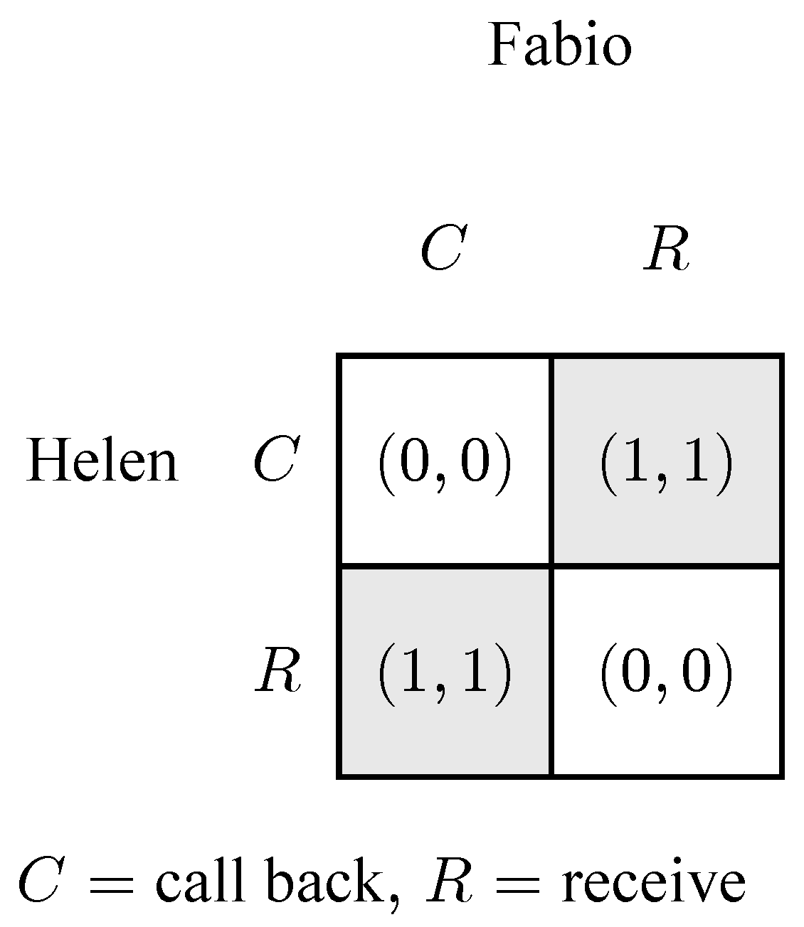
- C when I am the original caller, and R otherwise.
can be salient for the agents involved because they take note of the fact that in past similar situations the original caller called back and in the main they disregard the other analogies between these similar situations.
Salience can originate from many different factors, but it is well established that the salience of a particular equilibrium or strategy is relative to a particular community and dependent upon the common background of this community.19 Why do some Ultimatum Game studies limit the Recipient pure strategy set to the threshold strategies? I conjecture that for the economists who design these studies, the threshold strategies form a salient strategy set. The idea of a minimally acceptable offer may have some psychological prominence for those who are accustomed to thinking of homo economicus, an individual of the sort who for whom generally “more is better than less” so that if he would accept at least , he would certainly accept for any . In the experimental studies where Recipient subjects are asked to give their minimum acceptable offers, the instructions they receive may contribute to the salience of the threshold strategy set for them since they presumably know all subjects receive these instructions. Therefore, what is part of the experimenters’ common background becomes part of the Recipient subjects’ common background.
However, I also suggest the threshold strategy set is not the only possible salient strategy set of an Ultimatum Game. I introduced the n-piece Range RUGs of Section 3 and Section 4 with an admittedly ulterior motive. I conjecture that some communities could regard the range strategies as salient because for the members of these communities the fact that a certain offer lies in one of a set of ranges of offers is psychologically prominent, where the ranges include but are not limited to the ranges of threshold strategies. As discussed in Section 4, the simulation results of the 10-piece Threshold RUG and the 10-piece Range RUG are similar, in that for both games the populations converge most often to equilibria more favorable to Recipients than the subgame perfect equilibrium. This finding is compatible with the results of the best-known Ultimatum Game laboratory experiments run with subjects from cultures having relatively high degrees of cooperative activity and market integration. Therefore, the evidence of these experiments is at least compatible with these subjects thinking their game is a Range Ultimatum Game, even though in many of these experiments they are cued to think of their game as a Threshold Ultimatum Game. Additionally, as noted in the Introduction, in Ultimatum Game experiments run with subjects from some other cultures, Proposers sometimes make hyperfair offers and Recipients sometimes reject hyperfair offers. Henrich et al. (2001), Henrich et al. (2005) and Henrich et al. (2014) report the results of some of these experiments. Henrich et al. (2014) report some particularly striking findings on a set of Ultimatum Games run on subjects from 14 different societies, including seven African, two Papua New Guinean, one Oceanic, one Siberian, three Latin American and one rural North American. In 10 of these societies, some Proposers made hyperfair offers. Additionally, in 10 of these societies, subjects who were asked to indicate which offers they would reject reported they would reject some hyperfair offers as well as some unfair offers. In a number of these societies the probability of reported intended rejection increases as the offer increases from 60% to 100% of the pie. Moreover, Henrich et al. (2001), Henrich et al. (2005) and Henrich et al. (2014) report that subjects from the Au and the Gnau populations of Papua New Guineaactually do reject both hyperfair and unfair offers with nearly equal frequency. Various explanations for this phenomenon of hyperfair punishment have been proposed. To give only one example, Gintis et al. (2005, p. 29) note that in Melanesian cultures one can seek higher status by making a large gift, and one might reject the offer of such a gift in order to avoid accepting the subordinate status that comes with accepting a large gift. So hyperfair punishment in Ultimatum Games might occur in some societies like the Au and Gnau societies because the Proposers and Recipients are applying norms of competitive gift-giving to their Ultimatum Game. However, whatever the explanation of hyperfair punishment might be, I propose that for those in cultures where hyperfair punishment is observed, range strategies, that include strategies that reject offers that are “too high” as well as “too low”, might be the salient strategies so that their Ultimatum Game is a Range RUG.
The evolutionary analysis of Section 4 shows that the final distribution of evolved equilibria in an Ultimatum Game depends in no small part upon which pure strategy set defines the Recipients’ pure strategies in this Ultimatum Game. The Section 4 analysis also at least suggests that for actual communities whose members learn by experience, if the community members regard a certain proper subset of the logically possible Recipient strategies as salient strategies then they can converge to equilibria where the Proposer is not being most greedy far more often than if “anything goes” for Recipients. Again, “less can be more” for Recipients in terms of the strategies they actually employ. In my opinion strategy salience in Ultimatum Games has not been considered directly before with the partial exception of studies that examine threshold strategies, and even these studies do not recognize that strategy salience is playing a role when the Recipients are encouraged to follow or even limited to following threshold strategies. As the possibilities describe above illustrate, the strategy set that the agents in an Ultimatum Game regard as salient, that is, as their strategy set, might vary markedly across communities according to a variety of background conditions. And which strategy set is their strategy set can markedly influence how agents learn to play their Ultimatum Game over time. Future work might explore which pure strategies in an Ultimatum Game are indeed salient for actual communities and how this strategy salience interacts with how they learn in repeated Ultimatum Games.
Funding
This research received no external funding.
Data Availability Statement
The raw data supporting the conclusions of this article will be made available by the author on request.
Acknowledgments
I thank Tianzhe Cozette Shen for her work in editing the submission version of this manuscript.
Conflicts of Interest
The author declares no conflicts of interest.
| 1 | In this round, all but one Proposer offered or more of the sum at stake, and this share was always at least 1 mark. The exceptional Proposer offered of 5 marks, and the Recipient spurned. Of the five cases where Recipients spurned an offer of at least 1 mark, in four of these cases, the Proposer offered or less. |
| 2 | Camerer (2003, p. 72) reports that market integration is an index that combines the existence of a national language, the existence of a labor market for cash wages, and the existence of farming of crops for cash. |
| 3 | Camerer (2003, p. 49) notes that cueing the subjects this way elicits information regarding likely responses to all offers. |
| 4 | In a survey of recent evolutionary game theory work on Ultimatum Games, Debové, Baumard, and André give a definition of a threshold strategy and then discuss all of the works of this survey in terms of this definition (Debove et al., 2016). |
| 5 | Here, I follow the practice of previous Ultimatum Game studies such as Roth and Erev (1995) and Gale et al. (1995) and refer to a Nash equilibrium where a Recipient accepts any positive offer as subgame perfect. In Section 3, I explain why I think this is a slight but harmless abuse of terminology. |
| 6 | In this paper I will limit my discussion to Ultimatum Games where Z is a finite set, which reflects the conditions of most Ultimatum Game experiments where the good at stake is a sum of money divisible up to only finitely many increments. Of course one can also define Continuous Ultimatum Games where Z = [0, 1] or some infinite proper subset of [0, 1]. |
| 7 | While the Proposer moves first, for strategic form representations, it is convenient to arrange the pure strategy profiles and payoff vectors in this manner, which, following the usual conventions of game theory, makes the Recipient the row player and the Proposer the column player in a strategic form representation of an Ultimatum Game. |
| 8 | If an Agent j in a game has the pure strategy set , then denotes a mixed or partially mixed strategy for Agent j, where Agent j chooses with probability . |
| 9 | denotes the column vector transpose of the ordered n-tuple . |
| 10 | In fact, in (1), one of the n equations is redundant, and in (2), one of the m equations is redundant because and are equivalent to probability distributions and are thus fully determined by of the equations of (1) and of the equations of (2). |
| 11 | The code of these simulators and the simulation data are available from the author upon request. |
| 12 | Some of my own preliminary simulations on Ultimatum Games confirm one of Gale et al.’s (1995) findings in their analysis. Gale et al. (1995) discovered that the Proposers and the Recipients can tend to learn very slowly according to their 2-population replicator dynamic models and only might reach a final limit after many cycles of learning. Similarly, in their reinforcement learning simulations, Roth and Erev (1995) found that Proposers and Recipients can learn only very slowly to reach an equilibrium in an Ultimatum Game, and in their simulations, they allow the reinforcement learning to run for time cycles. In some preliminary simulations, I also found that the Proposers and the Recipients tend to learn slowly according to (1) and (2), which is why I chose the high number of 5000 time cycles for each orbit for the simulations discussed in this paper. |
| 13 | Interestingly, Gale et al. (1995) acknowledge that the full set of possible Recipient strategies are functions of the form , and they note that this is an unmanageably large strategy set. They immediately limit Recipient pure strategies to the 40 threshold strategies, resulting in a Threshold RUG. Indeed, the corresponding Unrestricted UG has pure Recipient strategies. |
| 14 | If one goes even further and considers or , then the results are degenerate games where the Recipient has no strategy option at all. If one sets , then the Recipient rejects all offers, so that there is effectively only one possible outcome where for any . If , then the Recipient can only accept all offers, and the resulting degenerate game is a Dictator Game. Experimental research on Dictator Games complements the experimental research on Ultimatum Games. Camerer (2003, pp. 56–58) summarizes the best-known results of Dictator Game experiments. |
| 15 | A proposition A is common knowledge among the members of a group if each member knows that all know A and knows that all can infer the consequences of this mutual knowledge. Lewis (1969, p. 56–57) presented one of the first analyses of common knowledge. |
| 16 | Note that, for each of these profiles, the Proposer’s and the Recipient’s pure strategies are parts of Nash equilibria. Therefore, each of these profiles is compatible with common knowledge of Bayesian rationality and the payoff structure of the game, the defining conditions of rationalizability. For example, for the nonequilibrium profile , and are corresponding Nash equilibria. Suppose the Proposer’s conjecture is that she believes with probability one that the Recipient will follow his part of and the Recipient’s conjecture is that he believes with probability one that the Proposer will follow her part of . Then is a best response for the Proposer and is a best response for the Recipient; therefore, is rationalizable. |
| 17 | See especially A Treatise of Human Nature (Hume, 1739–1740/2000), Book III, Part I, Sections 1–3 and An Enquiry Concerning the Principles of Morals (Hume, 1751/1998), Section III, Part II and Appendix III. |
| 18 | |
| 19 |
References
- Aumann, R. J. (1974). Subjectivity and correlation in randomized strategies. Journal of Mathematical Economics, 1(1), 67–96. [Google Scholar]
- Aumann, R. J. (1987). Correlated equilibrium as an expression of Bayesian rationality. Econometrica: Journal of the Econometric Society, 55, 1–18. [Google Scholar]
- Bernheim, B. D. (1984). Rationalizable strategic behavior. Econometrica: Journal of the Econometric Society, 52, 1007–1028. [Google Scholar]
- Bicchieri, C. (2005). The grammar of society: The nature and dynamics of social norms. Cambridge University Press. [Google Scholar]
- Camerer, C. (2003). Behavioral game theory: Experiments in strategic interaction. Princeton University Press. [Google Scholar]
- Debove, S., Baumard, N., & André, J.-B. (2016). Models of the evolution of fairness in the ultimatum game: A review and classification. Evolution and Human Behavior, 37(3), 245–254. [Google Scholar]
- Fehr, E., & Schmidt, K. M. (1999). A theory of fairness, competition, and cooperation. The Quarterly Journal of Economics, 114(3), 817–868. [Google Scholar]
- Gale, J., Binmore, K. G., & Samuelson, L. (1995). Learning to be imperfect: The ultimatum game. Games and Economic Behavior, 8(1), 56–90. [Google Scholar]
- Gintis, H., Bowles, S., Boyd, R., & Fehr, E. (2005). Moral sentiments and material interests: Origins, evidence, and consequences. In Moral sentiments and material interests: The foundations of cooperation in economic life. The MIT Press. [Google Scholar] [CrossRef]
- Güth, W., & Kocher, M. G. (2014). More than thirty years of ultimatum bargaining experiments: Motives, variations, and a survey of the recent literature. Journal of Economic Behavior & Organization, 108, 396–409. [Google Scholar]
- Güth, W., Schmittberger, R., & Schwarze, B. (1982). An experimental analysis of ultimatum bargaining. Journal of Economic Behavior & Organization, 3(4), 367–388. [Google Scholar]
- Harms, W. (1997). Evolution and ultimatum bargaining. Theory and Decision, 42, 147–175. [Google Scholar]
- Henrich, J., Boyd, R., Bowles, S., Camerer, C., Fehr, E., Gintis, H., & McElreath, R. (2001). In search of homo economicus: Behavioral experiments in 15 small-scale societies. American Economic Review, 91(2), 73–78. [Google Scholar]
- Henrich, J., Boyd, R., Bowles, S., Camerer, C., Fehr, E., Gintis, H., McElreath, R., Alvard, M., Barr, A., Ensminger, J., Henrich, N. S., Hill, K., Gil-White, F., Gurven, M., Marlowe, F. W., & Tracer, D. (2005). “Economic man” in cross-cultural perspective: Behavioral experiments in 15 small-scale societies. Behavioral and Brain Sciences, 28(6), 795–815. [Google Scholar] [PubMed]
- Henrich, J., Ensminger, J., Barr, A., & McElreath, R. (2014). Major empirical results: Markets, religion, community size, and the evolution of fairness and punishment. In Experimenting with social norms: Fairness and punishment in cross-cultural perspective (pp. 89–148). Russell Sage Foundation. [Google Scholar]
- Hume, D. (1998). David hume: An enquiry concerning the principles of morals: A critical edition (T. L. Beauchamp, Ed.). Clarendon Press. (Original work published 1751). [Google Scholar]
- Hume, D. (2000). A treatise of human nature: Being an attempt to introduce the experimental method of reasoning into moral subjects (D. F. Norton, & M. J. Norton, Eds.). Oxford University Press. (Original work published 1739–1740). [Google Scholar]
- Lewis, D. K. (1969). Convention: A philosophical study. Wiley-Blackwell. [Google Scholar]
- Mehta, J., Starmer, C., & Sugden, R. (1992). An experimental investigation of focal points in coordination and bargaining: Some preliminary results. In Decision making under risk and uncertainty: New models and empirical findings (pp. 211–219). Springer. [Google Scholar]
- Mehta, J., Starmer, C., & Sugden, R. (1994a). Focal points in pure coordination games: An experimental investigation. Theory and Decision, 36, 163–185. [Google Scholar]
- Mehta, J., Starmer, C., & Sugden, R. (1994b). The nature of salience: An experimental investigation of pure coordination games. The American Economic Review, 84(3), 658–673. [Google Scholar]
- Pearce, D. G. (1984). Rationalizable strategic behavior and the problem of perfection. Econometrica: Journal of the Econometric Society, 52, 1029–1050. [Google Scholar]
- Roth, A. E., & Erev, I. (1995). Learning in extensive-form games: Experimental data and simple dynamic models in the intermediate term. Games and Economic Behavior, 8(1), 164–212. [Google Scholar]
- Schelling, T. C. (1980). The strategy of conflict: With a new preface by the author. Harvard University Press. [Google Scholar]
- Skyrms, B. (2014). Evolution of the social contract (2nd ed.). Cambridge University Press. [Google Scholar]
- Vanderschraaf, P. (1995). Convention as correlated equilibrium. Erkenntnis, 42(1), 65–87. [Google Scholar]
- Vanderschraaf, P. (2018). Strategic justice: Convention and problems of balancing divergent interests. Oxford University Press. [Google Scholar]
- Young, H. P. (1998). Individual strategy and social structure: An evolutionary theory of institutions. Princeton University Press. [Google Scholar]
Figure 5.
Five-piece singleton RUG (pure strategy Nash equilibria shaded).

Figure 7.
Final state Proposer strategy distributions, simulations of replicator dynamics applied to 5-piece Ultimatum Games (proposer strategies in terms of number of pieces offered).
Figure 7.
Final state Proposer strategy distributions, simulations of replicator dynamics applied to 5-piece Ultimatum Games (proposer strategies in terms of number of pieces offered).
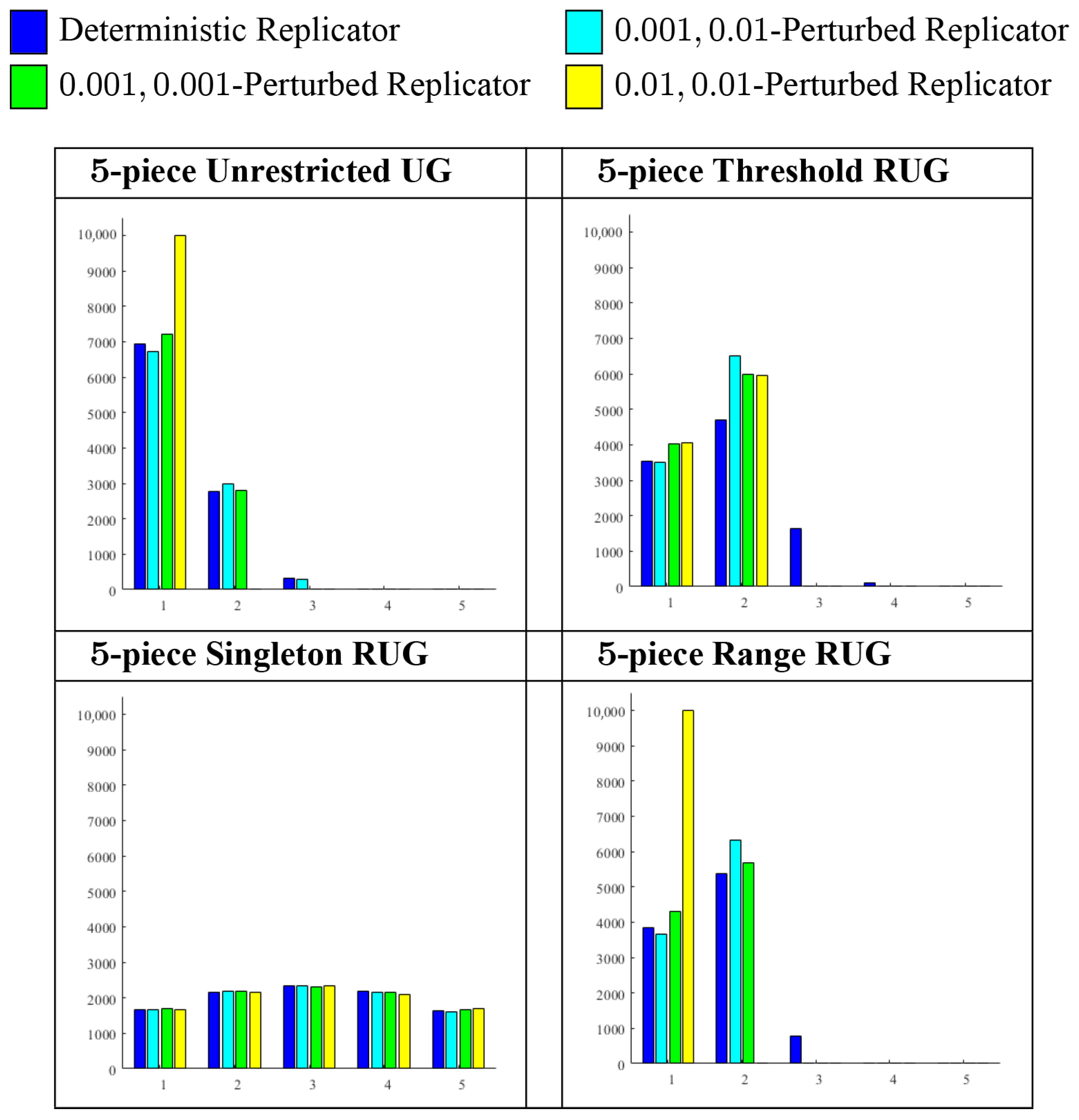
Figure 8.
Final State Proposer strategy distributions, simulations of 0.001, 0.01 perturbed replicator applied to 10-piece Ultimatum Games (Proposer strategies in terms of number of pieces offered).
Figure 8.
Final State Proposer strategy distributions, simulations of 0.001, 0.01 perturbed replicator applied to 10-piece Ultimatum Games (Proposer strategies in terms of number of pieces offered).


Table 1.
Convergence rates of 0.99, 0.99, simulations of replicator dynamics applied to 5-piece Ultimatum Games.
Table 1.
Convergence rates of 0.99, 0.99, simulations of replicator dynamics applied to 5-piece Ultimatum Games.
| , -Perturbed Replicator Dynamics | ||||
|---|---|---|---|---|
| Unrestricted UG | 1.0 | 1.0 | 0.9999 | 1.0 |
| Threshold RUG | 1.0 | 1.0 | 1.0 | 0.9999 |
| Singleton RUG | 1.0 | 1.0 | 1.0 | 1.0 |
| Range RUG | 1.0 | 1.0 | 1.0 | 1.0 |
Table 2.
Sizes of basins of attraction, simulations of replicator dynamics applied to 5-piece Ultimatum Games.
Table 2.
Sizes of basins of attraction, simulations of replicator dynamics applied to 5-piece Ultimatum Games.
| , -Perturbed Replicator Dynamics | |||||
|---|---|---|---|---|---|
| Proposer | |||||
| Offer | |||||
| Unrestricted UG | 0.6298 | 0.6712 | 0.7206 | 1.0 | |
| 0.2756 | 0.2982 | 0.2793 | 0.0 | ||
| 0.0314 | 0.0306 | 0.0 | 0.0 | ||
| 0.0002 | 0.0 | 0.0 | 0.0 | ||
| 0.0 | 0.0 | 0.0 | 0.0 | ||
| Threshold RUG | 0.3540 | 0.3495 | 0.4030 | 0.4095 | |
| 0.4709 | 0.6505 | 0.5970 | 0.5954 | ||
| 0.1643 | 0.0 | 0.0 | 0.0 | ||
| 0.0108 | 0.0 | 0.0 | 0.0 | ||
| 0.0 | 0.0 | 0.0 | 0.0 | ||
| Singleton RUG | 0.1637 | 0.1622 | 0.1670 | 0.1706 | |
| 0.2193 | 0.2173 | 0.2147 | 0.2104 | ||
| 0.2328 | 0.2339 | 0.2306 | 0.2355 | ||
| 0.2170 | 0.2187 | 0.2185 | 0.2169 | ||
| 0.1672 | 0.1679 | 0.1692 | 0.1666 | ||
| Range RUG | 0.3851 | 0.3667 | 0.4314 | 1.0 | |
| 0.5363 | 0.6333 | 0.5686 | 0.0 | ||
| 0.0767 | 0.0 | 0.0 | 0.0 | ||
| 0.0019 | 0.0 | 0.0 | 0.0 | ||
| 0.0 | 0.0 | 0.0 | 0.0 | ||
Table 3.
Convergence rates of 0.99, 0.99, simulations of replicator dynamics applied to 10-piece Ultimatum Games.
Table 3.
Convergence rates of 0.99, 0.99, simulations of replicator dynamics applied to 10-piece Ultimatum Games.
| , -Perturbed Replicator Dynamics | ||||
|---|---|---|---|---|
| Unrestricted UG | 0.9996 | 0.9998 | 0.9998 | 0.9999 |
| Threshold RUG | 1.0 | 1.0 | 0.9995 | 1.0 |
| Singleton RUG | 0.9780 | 1.0 | 1.0 | 1.0 |
| Range RUG | 0.9989 | 0.9988 | 0.9995 | 0.9988 |
Table 4.
Sizes of basins of attraction, simulations of replicator dynamics applied to 10-piece Ultimatum Games.
Table 4.
Sizes of basins of attraction, simulations of replicator dynamics applied to 10-piece Ultimatum Games.
| , -Perturbed Replicator Dynamics | |||||
|---|---|---|---|---|---|
| Proposer | |||||
| Offer | |||||
| Unrestricted UG | 0.4714 | 0.4515 | 0.4622 | 0.4578 | |
| 0.3448 | 0.3627 | 0.3614 | 0.3609 | ||
| 0.1544 | 0.1501 | 0.1530 | 0.1575 | ||
| 0.0290 | 0.0272 | 0.0231 | 0.0236 | ||
| 0.0 | 0.0005 | 0.0001 | 0.0001 | ||
| 0.0 | 0.0 | 0.0 | 0.0 | ||
| 0.0 | 0.0 | 0.0 | 0.0 | ||
| 0.0 | 0.0 | 0.0 | 0.0 | ||
| 0.0 | 0.0 | 0.0 | 0.0 | ||
| 0.0 | 0.0 | 0.0 | 0.0 | ||
| Threshold RUG | 0.1050 | 0.1000 | 0.1052 | 0.1076 | |
| 0.3168 | 0.3163 | 0.4139 | 0.8924 | ||
| 0.3464 | 0.3529 | 0.4788 | 0.0 | ||
| 0.1846 | 0.2308 | 0.0016 | 0.0 | ||
| 0.0430 | 0.0 | 0.0 | 0.0 | ||
| 0.0041 | 0.0 | 0.0 | 0.0 | ||
| 0.0001 | 0.0 | 0.0 | 0.0 | ||
| 0.0 | 0.0 | 0.0 | 0.0 | ||
| 0.0 | 0.0 | 0.0 | 0.0 | ||
| 0.0 | 0.0 | 0.0 | 0.0 | ||
| Singleton RUG | 0.0066 | 0.0686 | 0.0672 | 0.0673 | |
| 0.0931 | 0.0986 | 0.0961 | 0.1003 | ||
| 0.1227 | 0.1208 | 0.1218 | 0.1252 | ||
| 0.1332 | 0.1355 | 0.1297 | 0.1377 | ||
| 0.1375 | 0.1367 | 0.1399 | 0.1363 | ||
| 0.1276 | 0.1297 | 0.1357 | 0.1348 | ||
| 0.1188 | 0.1278 | 0.1277 | 0.1218 | ||
| 0.1047 | 0.1084 | 0.1036 | 0.1036 | ||
| 0.0744 | 0.0739 | 0.0783 | 0.0730 | ||
| 0.0 | 0.0 | 0.0 | 0.0 | ||
| Range RUG | 0.0231 | 0.0215 | 0.1052 | 0.0220 | |
| 0.4285 | 0.4098 | 0.4139 | 0.9768 | ||
| 0.4412 | 0.4697 | 0.4788 | 0.0 | ||
| 0.0998 | 0.0978 | 0.0016 | 0.0 | ||
| 0.0062 | 0.0 | 0.0 | 0.0 | ||
| 0.0001 | 0.0 | 0.0 | 0.0 | ||
| 0.0 | 0.0 | 0.0 | 0.0 | ||
| 0.0 | 0.0 | 0.0 | 0.0 | ||
| 0.0 | 0.0 | 0.0 | 0.0 | ||
| 0.0 | 0.0 | 0.0 | 0.0 | ||
Disclaimer/Publisher’s Note: The statements, opinions and data contained in all publications are solely those of the individual author(s) and contributor(s) and not of MDPI and/or the editor(s). MDPI and/or the editor(s) disclaim responsibility for any injury to people or property resulting from any ideas, methods, instructions or products referred to in the content. |
© 2025 by the author. Licensee MDPI, Basel, Switzerland. This article is an open access article distributed under the terms and conditions of the Creative Commons Attribution (CC BY) license (https://creativecommons.org/licenses/by/4.0/).
Share and Cite
MDPI and ACS Style
Vanderschraaf, P.P. “Anything Goes” in an Ultimatum Game? Games 2025, 16, 36. https://doi.org/10.3390/g16040036
AMA Style
Vanderschraaf PP. “Anything Goes” in an Ultimatum Game? Games. 2025; 16(4):36. https://doi.org/10.3390/g16040036
Chicago/Turabian StyleVanderschraaf, Peter Paul. 2025. "“Anything Goes” in an Ultimatum Game?" Games 16, no. 4: 36. https://doi.org/10.3390/g16040036
APA StyleVanderschraaf, P. P. (2025). “Anything Goes” in an Ultimatum Game? Games, 16(4), 36. https://doi.org/10.3390/g16040036
Note that from the first issue of 2016, this journal uses article numbers instead of page numbers. See further details here.