1. Introduction
Insider trading has long been a key research topic in financial economics and legal regulation. The majority of traditional studies focus on the information asymmetry of insider trading and its impact on market efficiency, as well as broader macro-level issues such as insider trading in the global economic environment (
Kamensky et al., 2020). While the increasing economic and political integration of markets continues to shape financial structures, information flows (
Alkharafi & Alsabah, 2025), and the strategies of traders, less attention has been paid to the role of individual heterogeneity among insider traders. In particular, the individual heterogeneity of insider traders, as rational decision-making subjects with information advantages, especially differences in risk attitudes, may influence the selection of trading strategies, market equilibrium price formation, and regulatory effectiveness. Insider traders should be risk-neutral in classical theoretical models like the
Kyle (
1985) model. However, traders can be risk-averse or risk-seeking due to personal characteristics, incentives, or variations in the market environment. Among other things,
Ausubel (
1990) suggests that risk-averse insider traders prefer to diversify their trades or shorten the period of holding their positions in order to avoid regulatory risk. Risk-averse insiders, on the other hand, maximize their informational advantage through leverage or more covert trading strategies to gain more returns. This heterogeneous risk mentality impacts not only individual trading behavior but also the rate at which the value of a financial instrument is integrated into its price and market liquidity. Market liquidity is a core attribute of financial markets, reflecting the ability of assets to be realized quickly at a reasonable price.
Amihud (
2002) portrays market liquidity through the four-dimensional indexes of market width, depth, elasticity, and immediacy. As a result, it is of research interest to investigate the impact of various types of insider traders on market liquidity.
Such problems can be traced back to
Kyle (
1985). The model assumes the existence of a risk-neutral insider trader with private information about the asset’s value, a risk-neutral market maker, and noise traders. The insider trader chooses the volume of trades based on profit maximization in a Nash equilibrium. Noise traders determine trading volumes through noise trading, which is based on their fears of hype or incomplete information. Therefore, the additional price fluctuations caused by noise trading do not reflect the true value of stocks. The market maker sets prices by observing the aggregate order flow. The pricing rule coefficient
represents the market depth parameter;
is used to measure the size of the market depth. Market depth measures how much a trader can buy or sell in a market without causing a significant change in the price. A person can jump in (trade a lot) without hitting the bottom (changing the price much) in deeper water.
The model derives the optimal insider trading strategy and market maker pricing rule by solving for the Nash equilibrium, revealing the dynamic value integration process that occurs in the price. Research has shown that the intensity of insider traders’ trades,
, is related to the precision of the information and the amount of market noise traded. The more precise the information (the smaller the
), or the larger the volume of noise trading (the larger the
), the more aggressively the insider trader will trade (the larger the
). The market depth parameter,
, is determined by the precision of the information and the volume of noise trading, suggesting that an increase in noise trading increases market depth.
Kyle (
1985) researched the trading strategies of insider traders, the linear pricing rules of market makers, the determinants of market depth, and the process of integrating value into price, providing the theoretical foundation for subsequent research on insider trading and market liquidity.
Subsequent research has been based on the
Kyle (
1985) model. For example,
Subrahmanyam (
1991) introduced risk-averse insider traders based on the
Kyle (
1985) model. It was found that market liquidity is non-monotonically related to the number of risk-averse insider traders, the degree of risk aversion of insider traders, and the accuracy of insider traders’ information, while the presence of risk-averse insider traders leads to a reduction in the volume of insider trading and a slower integration of value into price. The
Holden and Subrahmanyam (
1992) model was then modified by introducing multiple insider traders to the
Kyle (
1985) model. This competition led to the release of information into the market more quickly, which affected price efficiency and market liquidity.
Holden and Subrahmanyam (
1994) extended the
Holden and Subrahmanyam (
1992) model further by introducing several risk-averse insider traders and extending the model from a single-period insider trading model to a multi-period trading model. The model was solved by backward recursion to obtain a unique linear equilibrium that satisfies the model. The results demonstrated that both monopolistic and competitive insider traders could trade quickly with insider information, resulting in a lower market depth initially, a significant increase later on, and a quicker integration of private information into the market price.
Foster and Viswanathan (
1996) further explored the modeling of multi-period insider trading in settings where several insider traders had access to diverse information.
Back et al. (
2000) investigated a continuous-time insider trading model conditional on the
Foster and Viswanathan (
1996) model and given a unique linear equilibrium under the condition of imperfect correlation of information signals.
Baruch (
2002) provided a continuous version of the
Holden and Subrahmanyam (
1994) model. In contrast,
Zhang (
2004) made the first effort to simulate the best strategy of risk-averse insider traders in the context of information disclosure based on
Huddart et al. (
2001).
Relevant research has continued to be conducted in recent years.
Daher et al. (
2020) extended
Kyle’s (
1985) model to two insider traders, one being risk-neutral and the other risk-averse. By comparing the works of
Tighe and Michener (
1994) (a risk-neutral insider trader model) and
Holden and Subrahmanyam (
1994) (a risk-averse insider trader model), the influence of different risk attitudes of insider traders on market depth and the speed at which value is integrated into prices was discovered. The relationship between risk aversion and market depth was derived. That is, the risk aversion coefficient increases with the increase in market depth. Furthermore, compared to the work of
Tighe and Michener (
1994), the market depth of this model has consistently been relatively low. This intuitively suggests that the participation of risk-averse insider traders weakens trading willingness, thereby reducing market depth. Compared to those of
Holden and Subrahmanyam (
1994), the results have become more complex and require discussion on a case-by-case basis.
Daher et al. (
2014) extended the
Kyle (
1985) model of the private information transaction of a single asset to a multi-asset strategic transaction under the competitive correlation of the product market and found that insiders would conduct cross-asset strategic transactions, the price influence matrix showed asymmetry, and the market liquidity significantly depended on the intensity of product competition.
Jiang and Liu (
2022) extended the
Kyle (
1985) model to the case of two insider traders, one risk-neutral trader and one risk-seeker, and examined the effect of their level of self-confidence as well as the strength of the private information flow on market stability.
Daher et al. (
2023) conclude that a market with asymmetric information has a unique equilibrium solution if the information structure and the traders’ strategies satisfy specific constraints.
Daher and Saleeby (
2023) extended the
Kyle (
1985) model to the case of two risk-neutral insider traders and investigated the effect of the insider trader’s internal signaling error term on linear equilibrium uniqueness.
Carré et al. (
2022) extended the
Kyle (
1985) model to situations in which insider traders may be subject to additional trading penalties that increase the size of their trades and described how effective insider trading penalties, from a regulator’s point of view, can be in terms of market liquidity and the speed of price incorporation into prices.
Through a review of the previous literature, the influence of herding behavior, investors’ cognitive bias, etc., on the market has been studied and confirmed. However, research on how the scale of risk-averse insider traders systematically acts on the market microstructure is relatively scarce. We have filled this gap by studying and examining the impact of insider traders’ mixed risk attitudes (risk-neutral vs. risk-averse) on the financial market. Our first contribution is that, based on the framework of
Daher et al. (
2020), this study extends the original model by incorporating one risk-neutral and one risk-averse insider trader into a hybrid model with multiple risk-neutral and risk-averse insider traders. Furthermore, as noted by
Dieci et al. (
2006), the number of risk-neutral and risk-averse insider traders characterizes market mood. The linear equilibrium of the market can help us to understand how the market reaches a stable state under different information and expectations and provide theoretical support for investment decisions, risk management, and policy design. Given this, our second contribution is that this paper derives the unique linear equilibrium of the model through backward recursion, and, based on this, the optimal strategy of insider traders and the pricing rules of market makers are analyzed to reveal the dynamic process by which value integrates into price. It has been discovered that the trading volume of risk-neutral insider traders is consistently higher than that of risk-averse insider traders, which is consistent with the intuition that risk-averse insider traders trade conservatively to reduce the danger of price volatility.
Daher et al. (
2020) focused on the impact of different risk attitudes of insider traders on market depth, whereas
Foucault et al. (
2023) revealed the role of market liquidity in the importance of financial markets. As a result, this article compares the market liquidity of three different market models: the model with multiple risk-neutral and multiple risk-averse insider traders, the market with only multiple risk-neutral insider traders, and the market with only multiple risk-averse insider traders. It is found when this paper’s model is compared to the model with risk-neutral insider traders only, that the market liquidity is higher in the model with risk-neutral insider traders only, which intuitively means that, due to the presence of multiple risk-averse insider traders in this paper’s model, it weakens the incentives to trade, which, in turn, reduces the liquidity of the market. However, when this paper’s model is compared to the model with risk-averse insider traders only, the situation becomes more complicated and market liquidity depends heavily on the number of risk-averse insider traders.
This paper is structured as follows:
Section 2 examines an equilibrium model with the presence of both multiple risk-neutral and risk-averse insider traders in the market, solves for the parameters that characterize the equilibrium, and analyzes the effect of the number of risk-averse insider traders on the market equilibrium.
Section 3 comparatively analyzes the parameters related to market liquidity in the model with multiple risk-neutral insider traders and the model with multiple risk-averse insider traders. In
Section 4, we conduct the plotting through numerical simulation. In
Section 5, the conclusions of the paper are drawn. The proofs are presented in
Appendix A.
2. The Model
Referring to
Kyle’s (
1985) model, it is assumed that there are four types of traders in the market:
risk-neutral insider traders,
risk-averse insider traders,
noise traders, and
risk-neutral market makers (
Daher et al., 2020). More market makers compete to suppress information monopolies and reduce the information advantage of insider traders, which is the same as the assumption of
Daher et al. (
2020). The liquidation value of a tradable risky asset in the market is a random variable
, which is normally distributed with mean
and variance
, i.e.,
∼
. Noise traders, representing investors who do not observe
, have a trading volume denoted by
, which is normally distributed with mean 0 and variance
, i.e.,
∼
. Assume that the random variables
and
are independent. Risk-averse insider traders use a negative exponential utility function (
Holden & Subrahmanyam, 1994), and this utility function is often used to describe the risk preference of economic entities, indicating that economic entities are risk-averse. As the level of wealth increases, marginal utility decreases; that is, the additional satisfaction brought by the increase in wealth will gradually decrease. This is in line with people’s usual attitude towards risk; that is, under the same expected return, they tend to choose the option with lower risk:
where
A is the risk aversion coefficient. The deeper the degree of risk aversion is, the larger
A is.
In a deal, the insider trader receives the asset liquidation value because risk-neutral insider traders have the advantage of non-public, important, and valuable information. This advantage enables them to convert the value of information into excess profits through precise timing and trading strategies in an information-asymmetrical market. Therefore, risk-neutral insider traders choose their trading volume by maximizing the expected profits. Risk-averse traders, due to the diminishing marginal utility of wealth, are more sensitive to risks and do not simply pursue high returns. On the contrary, they rely on the expected utility function to find the optimal trading strategy that balances returns and risks in order to maximize their personal economic interests. Therefore, risk-averse insider traders determine their trading volume through maximizing the utility function. Moreover, insider traders are unaware of each other’s knowledge. In a semi-strong efficient market, market makers price based on the total order flow . Through the signal extraction function of the order flow, they decode the private information of market participants into public prices. While playing the role of a liquidity provider, they achieve a zero-expected loss equilibrium under risk neutrality. The market maker cannot view the separate values , , and .
The profits for each of the two types of insider traders are as follows:
.
Definition 1. The Nash equilibrium is the vector formed by three functions :
(a) Profit maximization by risk-neutral insider traders,for any ; (b) The maximization of the negative utility function of risk-averse insider traders,for any ; (c) Under semi-strong efficient market conditions, pricing rules satisfyThe equilibrium is linear if there exist constants μ and λ with the form The adoption of a linear pricing function by market makers is a mathematical necessity of Bayesian inference under the assumption of normal distribution, and it is also the simplest solvable form for the interaction between informed traders and market makers’ strategies to reach equilibrium. It balances information efficiency, operational feasibility, and risk control, and is the standard modeling paradigm of market microstructure theory.
Based on the above conditions, we obtain the following equilibrium model, in which the meaning of each parameter symbol is shown in
Table 1 and the definition of each variable is shown in
Table 2.
Proposition 1. A linear equilibrium exists and is unique in the presence of risk-neutral and risk-averse insider traders. It is characterized by the following:
(i) and
(ii), and the parameter λ is satisfied: The following lemma is obtained from Proposition 1:
Lemma 1. When the number of risk-averse insider traders tends to be infinite, risk-averse insider traders do not tend to trade, which is equivalent to only risk-neutral insider traders trading in the market. If the number of risk-neutral insider traders , the trading volume is the same as the monopoly trading volume of Kyle (1985). When , the trading volume and the two coefficients of the pricing equation are the same as those of Daher et al. (2020). It should be noted that models with mixed risk attitudes affect equilibrium trading orders. Proposition 1 suggests that the trading volume is asymmetric across the two risk attitudes. Specifically, risk-neutral insider traders trade more than risk-averse insider traders. Although both insider traders are fully aware of the value of risky assets, we note that risk-neutral insider traders dominate risk-averse insider traders in terms of trading. Intuitively, this result is related to the fact that risk-averse insider traders trade less aggressively than risk-neutral insider traders.
It can also be observed that the number of risk-averse insider traders has a direct impact on the calculation of the equilibrium results. More specifically, there is a direct effect on the market liquidity parameter
. Indeed, considering an insider trader in
Kyle (
1985) is risk-neutral, there is an explicit solution for the market liquidity parameter. However, when the insider traders are risk-averse, the market liquidity parameter
is a solution to a quadratic equation. Thus, we can obtain the relationship between
and
through differentiation, and the next lemma (Lemma 2) reveals the relationship between the two.
Lemma 2. where is the solution of a monic cubic polynomial concerning λ. Due to the complexity of the result of the computation, the exact form of the point will not be given here. Lemma 2 shows that the relationship between and is not monotonic, and the effect between the two values can only be observed for different ranges of . What is known, however, is that can take its maximum value , and the number of risk-averse insider traders tends to zero.
In the following section, the market liquidity parameter of the hybrid model is compared to the market liquidity parameter in the model of the market with only risk-neutral insider traders and the market liquidity parameter in the model of the market with only risk-averse insider traders, respectively.
3. Comparative Analysis
Before presenting the conclusions, we will calculate each parameter in the models with only risk-neutral insider traders and only risk-averse insider traders in the market, respectively, through the equilibrium conditions of Definition 1.
Proposition 2. When there are risk-neutral insider traders, N3 noise traders, and risk-neutral market makers in the market, the Nash equilibrium is given by the following:
(i) Profit maximization:
(ii)
where , Proposition 3. When there are risk-averse traders, N3 noise traders, and risk-neutral market makers in the market, the Nash equilibrium is given by the following:
(i) The maximization of the negative utility function:
(ii) , where is the unique positive root of the next quadratic equation:
The technique of proving Propositions 2 and 3 is parallel to Proposition 1; hence, it is omitted here.
The above two propositions provide help for the subsequent graphing as well as the proof of Lemma 3.
Lemma 3. The λ in this paper’s model is always lower than the market liquidity parameter of the model where insider traders are only risk-neutral (). However, compared to the market liquidity parameter () of the model with only risk-averse insider traders, the magnitude relationship depends on the number of risk-averse insider traders:
(a)
(b) There exists a risk-averse number of insider traders such thatwhere . Lemma 3 shows the effect of different risk attitudes on , the market liquidity parameter. In part (a) of Lemma 3, it is found that the addition of risk-averse insider traders to the market has an impact on market liquidity compared to a market with only risk-neutral insider traders. The results show that the market liquidity parameter in the model with mixed risk attitudes is smaller than that in the model with only risk-neutral insider traders in the market . The market can trade faster and at reasonable prices when there are only risk-neutral insider traders.
The following table systematically compares the trading volumes and market liquidity of four different models to more intuitively demonstrate the differences among models composed of different trading entities.
Based on Proposition 1 and Proposition 2 as well as the
Daher et al. (
2020) model, we present the trading volume and market liquidity parameters of each insider trader in
Table 3.
From
Table 3, we find that the trading volume of risk-neutral insider traders is greater than that of risk-averse insider traders in the two types of insider trader models with mixed risk attitudes. This result is consistent with intuition; that is, the trading intensity of risk-averse insider traders is not high, and therefore the trading volume is small. Meanwhile, when
, the trading volume and market liquidity parameter equations of multiple insider trader models with mixed risk attitudes correspond equally to those of the model with one risk-neutral and one risk-averse insider trader.
In the following section, we conduct numerical simulations to generate visualized results, which are then systematically analyzed to validate the key findings further.
4. Numerical Simulation
It is also important to note that, during the plotting process, is regarded as a continuous variable.
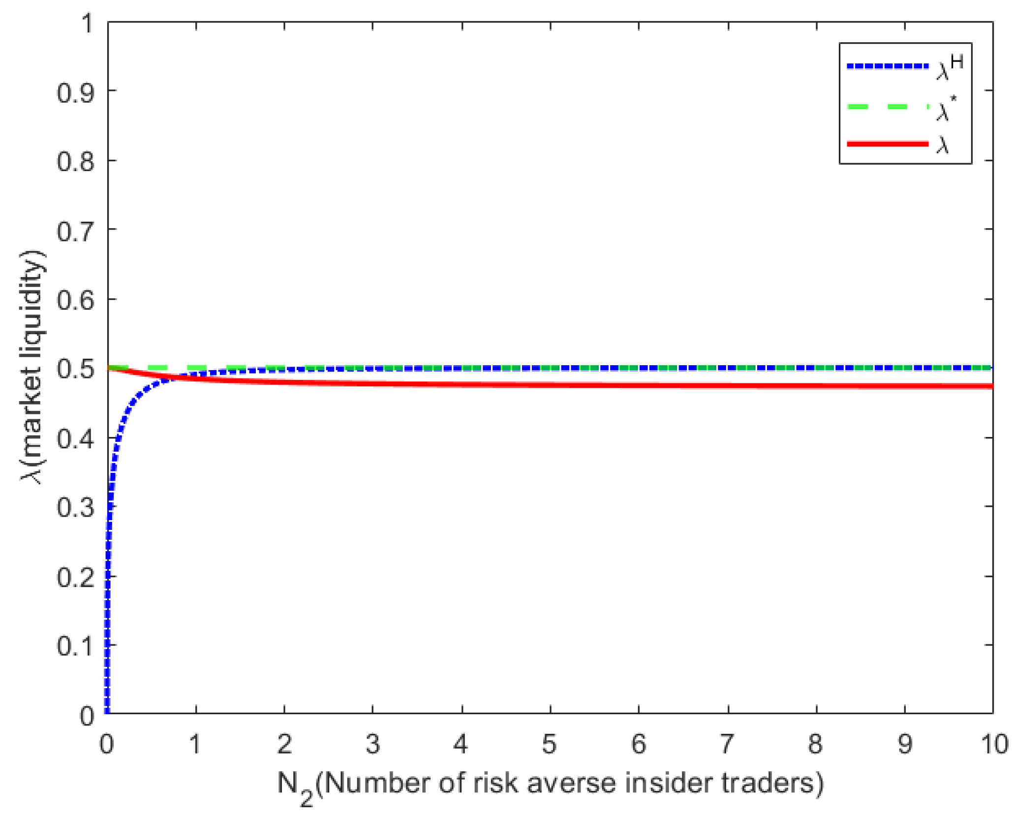
Figure 1 shows the variation of market liquidity parameter
with the number of risk-averse insider traders. It can be seen that the market liquidity parameter
is constant when the insider traders are all risk-neutral. Meanwhile, by comparing the model of mixed-risk insider traders with the model where only risk-averse insider traders exist in the market, it is concluded that, when the number of risk-averse insider traders reaches a certain level, the market liquidity in the model with only risk-averse insider traders is higher, and thus the market depth is smaller. This suggests that risk-neutral insider traders contribute to market depth. This conclusion is consistent with intuition: risk-averse insider traders tend to avoid trading, weakening market depth. This finding is consistent with the intuition that risk-averse insider traders will engage in aversive behavior towards trades, thus diminishing market depth. Therefore, the number of risk-averse insider traders is the main factor affecting market depth.
Figure 2 shows the variation of market liquidity parameter
with the number of risk-averse insider traders under different risk aversion coefficients. By observing
Figure 2, it can be seen that, as the risk aversion coefficient A increases, the intersection of
and
, which is the critical value of
in Lemma 3, becomes greater. However, regardless of the value of A, the overall direction of the curves
and
is roughly unchanged, indicating that the increase in the risk aversion coefficient A has little effect on the value of
in each curve. It is indicated that, when multiple risk-averse insider traders coexist, market liquidity is not sensitive to the degree of risk aversion of insider traders, while the number of risk-averse insider traders is the key factor affecting market liquidity. The increase in the number of risk-averse insider traders has weakened the impact of each trader’s degree of risk aversion on market liquidity. Therefore, in the stock market, from the perspective of regulators, one should pay more attention to the changes in the number of risk-averse insider traders.
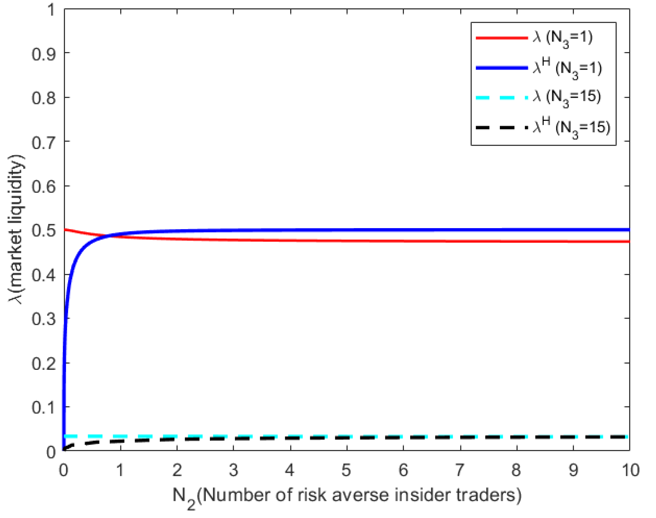
Figure 3 shows the variation of market liquidity parameter
with the number of risk-averse insider traders under different numbers of noise traders. It can be seen that the value of
decreases with an increase in
. Therefore, the following conclusions can be roughly obtained: Market liquidity weakens with the increase in the number of noise traders, and, thus, market depth increases with the increase in the number of noise traders, which is consistent with the conclusion obtained by
Kyle (
1985). Moreover, the intersection of
and
, the critical value
in Lemma 3, hardly varies with the increase in the number of noise traders
.
5. Conclusions
This paper studies and examines the impact of insider traders’ mixed risk attitudes (risk-neutral vs. risk-averse) on the financial market. The analysis shows that the number of risk-averse insider traders significantly impacts the equilibrium outcome. In the study, it is concluded that the number of risk-averse insider traders has a decreasing and then increasing relationship with market liquidity; that is, within a specific range, market liquidity decreases as the number of risk-averse insider traders increases, and, conversely, within another range, market liquidity increases as the number of risk-averse insider traders increases. Meanwhile, it is found that the market depth after the participation of risk-averse insider traders is more profound than that when only risk-neutral insider traders exist in the market. It indicates that the conservative trading strategies of risk-averse insider traders mitigate the impact of concentrated information releases on prices and, at the same time, may prompt market makers to provide more liquidity to address covert trading behaviors.
When the number of risk-averse insiders is small, their conservative trading strategies will reduce market liquidity. When the number exceeds the critical value, their progressive trading and risk diversification demands will instead enhance market depth. This phenomenon reveals that the relationship between market liquidity and information asymmetry is not one-sided. The differences in traders’ risk preferences will indirectly affect market stability.
This discovery reminds regulatory authorities that, first, the quantity threshold should be precisely regulated: regulators need to identify liquidity inflection points (such as through monitoring the risk appetite of order flows) and dynamically adjust the access scale of insider traders. Second, it reminds regulatory authorities to upgrade information disclosure: to require institutions to publicly disclose the range of risk aversion coefficients to assist market makers in optimizing pricing models and balancing information efficiency and liquidity. Finally, the incentive compatibility mechanism is designed to achieve the dual goals of market stability and efficiency.
The shortcomings of this article lie in the following: First, it is unable to provide an accurate value to determine the monotonic range of market liquidity and the number of risk-averse insider traders. Second, we assume that market makers can receive public signals and set prices based on these signals, as well as the total order flow, to study market liquidity.


