Article

Mobility Comparisons: Theoretical Definitions and People’s Perceptions

by
Michele Bernasconi
1,*,
Giulio Cinquanta
1,
Valentino Dardanoni
2 and
Vincenzo Prete
3
1
Department of Economics, University Ca’ Foscari of Venice, Cannareggio 873, 30121 Venezia, Italy
2
Department of Economics, Business and Statistics, University of Palermo, Ed. 13, Viale delle Scienze, 90128 Palermo, Italy
3
Department of Law, University of Palermo, Piazza Bologni 8, 90128 Palermo, Italy
*
Author to whom correspondence should be addressed.
Games 2025, 16(3), 24; https://doi.org/10.3390/g16030024
Submission received: 1 March 2025 / Revised: 2 May 2025 / Accepted: 6 May 2025 / Published: 8 May 2025
(This article belongs to the Section Behavioral and Experimental Game Theory)

Abstract

:
Comparing mobility is an important but controversial issue. In this paper, we argue that in a specific and relevant case, there exists a univocal and non-controversial definition of greater (exchange) mobility that allows for unambiguous comparisons. We conducted a questionnaire experiment to investigate whether people’s perceptions of social mobility align with this definition, and we found that people’s choices are broadly in line with the theoretical predictions.

1. Introduction

Understanding how people perceive social mobility—and how they judge one society to be more mobile than another—is crucial for explaining a range of social, economic, and political behaviors. Individuals assess risks in terms of potential gains or losses, much like voters form expectations about their prospects for upward or downward mobility. These perceptions, in turn, influence political preferences and support for institutional change (Acemoglu et al., 2018; Benabou & Ok, 2001).
Social mobility has important implications for both economic and political outcomes. In theoretical models, low mobility is associated with exclusionary policy preferences, religious revivalism, and resistance to institutional reform (Binzel & Carvalho, 2017; Uchida, 2018). More broadly, the way people perceive mobility shapes long-run dynamics such as strategic stability, path dependence, and intergroup interactions (Acemoglu et al., 2021). Preferences for redistribution, for instance, are known to depend on beliefs about mobility: when individuals perceive mobility to be high, support for redistribution tends to decline, as success is attributed primarily to personal effort and inequality is viewed as justifiable (Alesina et al., 2020; Fehr & Vollmann, 2022; Mengel & Weidenholzer, 2023).
Yet recent empirical research suggests that people systematically misperceive the actual level of social mobility. Upward mobility is often overestimated, while downward mobility is underestimated (Alesina & La Ferrara, 2005; Davidai, 2018; Davidai & Gilovich, 2015). These misperceptions may contribute to the puzzling negative correlation between inequality and mobility observed in the Great Gatsby Curve (Corak, 2013).
This raises a central question: are these misperceptions rooted in the ambiguity of how mobility is defined, or are they shaped more fundamentally by individual beliefs and subjective judgment? In this paper, we explore this question by focusing on comparisons of mobility for which there exists a clear, objective, and non-controversial criterion of what constitutes ‘greater mobility’.
Despite the crucial role of social mobility in several economic and social domains, the measurement of mobility is a highly controversial issue. Whether it is considered from an intragenerational or intergenerational perspective, social mobility remains a multifaceted concept. Researchers from different disciplines provide different definitions and indicators (Atkinson & Bourguignon, 1982; Benabou & Ok, 2001; Chakravarty et al., 1985; Cowell & Flachaire, 2018; D’Agostino & Dardanoni, 2009; Dardanoni, 1993; Fields, 2019; Fields & Ok, 1996; Gottschalk & Spolaore, 2002; Jäntti & Jenkins, 2015; Markandya, 1984; Van de gaer et al., 2001). The multifaceted nature of mobility also explains the considerable confusion about what higher mobility precisely means. Sociologists have provided a well-known definition of two aspects of interest in the mobility analysis: structural mobility and exchange mobility. For example, consider the social change experienced by a country following a period of economic growth, during which the number of high-status positions available for the generation of children significantly increases relative to those available for their parents. Structural mobility refers to the difference in the availability of high-status positions between parents and children. In contrast, exchange mobility focuses on the changes in social status between parents and children, that is, the extent to which children’s status depends on that of their parents.1
In this paper, we focus on exchange mobility. To isolate pure exchange mobility, we consider comparing mobility structures within the Fréchet class, i.e., mobility structures with the same marginal distributions (Fréchet, 1951). More specifically, the equality of marginals implies that the parents’ marginal distribution is the same in the two societies being compared, and the same holds for children’s marginal distributions, which may differ from those of the parents but do not vary between the two societies being compared. Furthermore, within the Fréchet class, we restrict our comparison to monotone mobility structures, where children from high-status parents always have stochastically better prospects than children from low-status parents. This assumption rules out comparisons involving scenarios that are theoretically admissible but unrealistic.2
In the first part of this paper, we argue that within this restricted class, there exists a univocal and non-controversial definition of greater (exchange) mobility that enables unambiguous mobility comparisons. We refer to this (partial) ordering as “positive dependence”.3 Then, we investigate the extent to which people’s perceptions of mobility align with the positive dependence ordering. This is achieved using a questionnaire experiment based on pairwise comparisons of different mobility scenarios, where respondents are asked to indicate which scenario they perceive as more mobile.
The approach adopted in this paper is closely related to the experimental method for inequality measurement pioneered by Amiel and Cowell (1992). In their work, the authors began with a set of widely accepted axioms for inequality comparisons and tested whether individuals in experimental settings agree with the resulting orderings. The analogy between inequality and mobility comparisons can be summarized as follows: (i) Lorenz curve comparisons (like positive dependence orderings in mobility) are meaningful only when societies have the same mean income—in our case, when marginal distributions are held constant; (ii) when income distributions share the same mean, the Lorenz criterion is broadly accepted because it corresponds to multiple alternative notions of greater inequality (Atkinson, 1970; Dasgupta et al., 1973; Kolm, 1976); similarly, within the Fréchet class, positive dependence provides an uncontroversial basis for mobility comparisons; (iii) nevertheless, just as individuals may reject Lorenz-consistent rankings in experimental inequality settings, they may also fail to align with the positive dependence ordering in mobility scenarios.
The key innovation of our paper is its emphasis on a precise definition of “pure exchange mobility,” achieved by comparing mobility structures within the Fréchet class and isolating the exchange component of social mobility by holding marginal distributions constant and thus removing the structural component. It then uniquely employs an experimental design to directly examine whether individuals’ perceptions of greater mobility align with this theoretically established definition, thus offering novel empirical insights into the intuitive comprehension of social mobility.
The rest of this paper is organized as follows: Section 2 introduces the theoretical framework and the positive dependence ordering. The questionnaire experiment and sample characteristics are presented in Section 3. Section 4 discusses the results, and Section 5 concludes the paper.

2. Mobility Comparisons

Social mobility in a society is typically represented by the joint distribution of two random variables: one indicating the social status of parents, and the other the status of their children (e.g., income quintiles, occupational categories). This joint distribution reflects two key components: the structural and exchange aspects of mobility. The structural component refers to generational changes in the availability of high-status positions; for example, shifts driven by economic growth. In contrast, the exchange component captures the degree to which families reallocate their relative positions along the social hierarchy. Both dimensions are encoded in a standard mobility table.
To illustrate this, consider the simplest case of a generic Society A, where parental and child status are each binary variables, taking values in the set { L , H } , denoting low and high status, respectively. The joint distribution of parent and child status, denoted by A ( P , C ) : R + 2 [ 0 , 1 ] , can be represented by the mobility matrix shown in Table 1.
Each cell in the table represents the joint probability of a specific parent–child status pairing. The row and column totals correspond to the marginal distributions A P and A C , which represent the overall distribution of status in the parent and child generations, respectively. Note that, in this binary framework, all mobility tables with the same values of C L and P L belong to the Fréchet class—that is, the set of joint distributions sharing the same marginals—and differ by only one parameter, a—the probability that a child from a low-status family remains low-status. In mobility analysis, changes in the marginals A P and A C are referred to as structural mobility, while the way in which these marginals are coupled to a joint distribution captures exchange mobility. In this simple case, exchange mobility is entirely governed by the association parameter a.
Furthermore, to avoid unrealistic comparisons, such as cases where children from high-status parents attain low status and vice versa, we consider mobility structures in the Fréchet class that are also monotone. This means we consider only those cases in which children from higher-status parents have better chances of attaining higher status than children from lower-status parents. In other words, the distribution of outcomes for children with high-status parents stochastically dominates that of children with low-status parents: they are more likely to reach higher positions at every level.
Let F ( P , C ) denote the monotone Fréchet class. Within this class, let A ( P , C ) and B ( P , C ) represent two joint distributions corresponding to the two hypothetical societies being compared. Table 2 illustrates the structure of a hypothetical comparison aligned with the one proposed by Questions 1–4 and 8–10 in our questionnaire experiment. In this setting—as shown in Section 3.1—it follows immediately that Society A always exhibits greater exchange mobility than Society B.4
When there are more than two social classes in the mobility tables within the Fréchet class, the mobility ordering requires that each element of the cumulative joint distribution in Society A—assumed to have greater exchange mobility—be less than or equal to the corresponding element in Society B. It follows that in all questions involving three social classes, the mobility tables can be ordered by directly comparing each element of the cumulative joint distributions. As an example, consider Question 5 (see Section 3.1), the cumulative joint distributions of which are displayed in Table 3—it can be immediately verified that Society A exhibits greater exchange mobility than Society B. The same logic applies to the mobility tables in Questions 6 and 7.
This definition of greater mobility establishes a partial order of mobility structures within F ( P , C ) , which we refer to as mobility dominance ordering, which is equivalent to the positive dependence ordering used in statistics (Atkinson & Bourguignon, 1982; Dardanoni, 1993).
In the administered questionnaire, the comparisons presented in Table 2 are translated into the format illustrated in Figure 1, which provides an example of a question comparing two societies with different levels of exchange mobility but identical structural mobility. Specifically, in both societies, the parents’ (upper panel) and the children’s (lower panel) generation have the same size, i.e., each generation consists of six individuals. However, the two societies exhibit different levels of exchange mobility. In Society A, three children from low-status parents remain in the low-status position, while the other three move to the higher-status position. The same dynamics apply to children from high-status parents: three of them remain in the same status as their parents, while the other three move down to the lower-status position. In Society B, instead, there is less exchange mobility. Specifically, only two children from low-status parents move to the high-status position, while the remaining four remain in the same social status class as their parents. According to the positive dependence ordering described earlier, we can say that A B , as the chance of moving from low-status to high-status position is greater in A relative to B. It is important to note that Society A represents the case of stochastic independence, which is the most mobile scenario used in our experiment questionnaire. Thus, following the above discussion, we formulate the hypothesis that participants completing the questionnaire should unambiguously recognize Society A as more mobile than Society B.

3. The Questionnaire Experiment

To test whether individuals perceive mobility in line with the concept of mobility dependence ordering, we conducted a questionnaire experiment. While the traditional approach in economics is to rely on revealed preference methods to infer unobserved factors from behavior, interest is now rapidly growing in using well-designed surveys to directly study factors, such as beliefs and perceptions, which preference methods may struggle to capture due to limited observable variation (Stantcheva, 2023). In the following, we describe the principles that guided the development of our questionnaire, while acknowledging some caveats.
The primary objective of the questionnaire was to ask respondents to compare two alternative mobility scenarios, where one is unambiguously more mobile than the other according to mobility dominance ordering; that is, it exhibits a higher level of exchange mobility while keeping the structural component constant. The underlying hypothesis is that individuals are able to recognize and correctly identify the scenario representing greater mobility, with people’s perceptions aligning with theoretical predictions.
The questionnaire was administered using Amazon Mechanical Turk (AMT), an online platform that enables rapid and cost-effective data collection from a diverse participant pool in the US. The AMT population does not reflect the general population, representing a limitation in terms of external validity and generalizability of the results (Aguinis et al., 2021). Some sampling biases identified in MTurk studies include the overrepresentation of younger, more educated individuals and participants from large urban areas, as well as white and non-Hispanic individuals. There is also a tendency to oversample Democratic-leaning respondents while underrepresenting Republicans and Independents. Additionally, as with most surveys, individuals at the extremes of the income distribution—both the very poor and the very wealthy—are typically underrepresented. Nevertheless, recent literature critically evaluating online survey methods has found that MTurk samples are generally more representative of the US population than traditional local convenience samples (Berinsky et al., 2012). Various prior studies have shown that AMT can be a valuable tool for exploring individuals’ views on issues related to distributive justice (Cappelen et al., 2018; Fisman et al., 2017; Kuziemko et al., 2015; Weinzierl, 2017). Given that this study represents one of the first attempts to investigate how people perceive a multifaceted concept such as intergenerational mobility, we consider AMT an appropriate starting point. Our objective was to precisely assess whether individuals’ perceptions align with a specific theoretical prediction, and AMT enables us to do so using a customizable and cost-efficient survey environment. It offers a more heterogeneous sample than university-based pools, even though certain demographics, such as students, may still be overrepresented. Participants receive a fixed monetary reward for completing the questionnaire, which is consistent with standard practices in studies of distributional perceptions. In such contexts, performance-based incentives are often difficult to implement effectively, but self-selected respondents are still likely to provide some thoughtful responses (Amiel et al., 2015; Fisman et al., 2021).5

3.1. The Questionnaire

Given the multidimensional nature of the social mobility concept, preparing a simple questionnaire is not an easy task. We followed Amiel (1999) and Amiel et al. (2015) and used “bus queues” of different colors to represent the income groups within the generation of parents and children, with colors identifying the dynasties. A set of instructions (reported in Appendix A.1) preceded the questionnaire (Cinquanta, 2020). Specifically, these instructions were designed to familiarize respondents with the concept of social mobility, defined as the process of socioeconomic status transition from the parents’ to the children’s generation. They also explain the questionnaire task, which involves choosing the most mobile societies in each of the proposed pairwise comparisons. In this regard, the instructions emphasize that parents’ socioeconomic status reflects only different life chances (circumstances), with no role for other factors such as effort and/or individual talent, which is assumed to be randomly distributed among parents’ and children’s generations. Finally, the instructions clarify that the incomes associated with each socioeconomic status are net of taxes and social transfers.
The questionnaire consists of 10 pairwise comparisons between two hypothetical societies (named A and B) displaying different levels of (exchange) mobility. These societies can be associated with mobility structures within the restricted class of monotone Fréchet matrices, where the equality of marginals holds for the marginal distributions of the parents in both alternative scenarios. The same holds for children’s marginals, although the marginals between parents and children may differ. Figure 1, described above, represents the first comparison in the questionnaire. The remaining pairwise comparisons introduce alternative scenarios with some variations.
More specifically, a subset of questions in the questionnaire focuses on comparisons involving extreme scenarios of intergenerational mobility. One such extreme is stochastic independence, which represents the most mobile scenario considered in our questionnaire. In this case, the economic status of the children is entirely unrelated to that of their parents (e.g., Society A in panel b of Figure 2). At the opposite extreme is immobility, where children’s outcomes are entirely determined by their parents’ status: all children from low-status parents remain in low-status positions, and likewise for those from high-status parents (e.g., Society B in both panels of Figure 2). In particular, in one question, we compare this immobile society with one that shows a certain degree of exchange mobility (Question 4—Figure 2a). In a second question, we present a direct comparison between the two polar cases: perfect immobility and stochastic independence (Question 10—Figure 2b). The underlying hypothesis is that people are able to correctly recognize the scenario exhibiting the higher level of mobility.
Questions 2 and 3 replicate the comparison presented in Question 1, but introduce changes in the income levels of the two generations, reflecting economic decline (Question 2—Figure 3a) or economic growth (Question 3—Figure 3b). It is important to note that the societies being compared still maintain the same level of structural mobility; the only difference between them is the level of exchange mobility. The rationale behind these questions is to assess whether individuals can still recognize the society with the higher mobility, even when the income support changes.
A third group of questions presents comparisons of mobility structures with three social classes and exchange mobility involving: (i) the middle and top classes (Question 5—Figure 4a); (ii) the bottom and middle classes (Question 6–Figure 4b); and (iii) the entire society (Question 7—Figure 4c). Comparing responses across this group of questions can provide insight into whether people’s perceptions of mobility change depending on which social classes are involved in the mobility process.
The final pair of questions explores scenarios in which the size of the dynasties differs (Question 8—Figure 5a) and where income growth is introduced (Question 9—Figure 5b). By incorporating these additional dimensions, the goal was to examine whether people could still recognize the society that exhibits the highest level of mobility.
These 10 pairwise comparisons were presented to a first group of participants in the questionnaire experiment. To minimize ordering effects, both the sequence of the questions and the positioning of the two alternative scenarios (Society A and Society B) were randomized across participants. A second group of participants received the same 10 comparisons; however, in this version, the level of mobility in the less mobile society (i.e., Society B) is further reduced in Questions 1–7, making the difference in mobility between the two scenarios more pronounced (see Appendix A.2). We refer to this modified version of the questionnaire as Q*.bis, to distinguish it from the standard version. Participants were randomly assigned to one of the two questionnaire versions—standard or Q*.bis.

3.2. The Sample

The questionnaire was administered in July 2019 to a sample of 258 respondents from the US, recruited through AMT. We excluded 16 respondents who failed to correctly answer three control questions designed to detect careless responses. The final sample included 242 respondents, with 115 assigned to the bis version of the questionnaire. On average, participants completed the survey in 11 min and received a standard participation fee of $1.
Table 4 reports summary statistics for the final sample,6 which includes a majority of male (62%) and white (72%) participants, with an average age of 35 years. Most respondents (58%) live alone, being either single or divorced. In terms of educational background, 12% hold a master’s degree, 49% a bachelor’s degree, and the remaining 39% possess a high school diploma. These demographic characteristics are broadly consistent with the general profile of the AMT population, which, as noted above, tends to be younger and more educated than the overall US population (Paolacci et al., 2010).7
The second panel of Table 4 provides additional information on respondents’ perceptions about their economic prospects relative to either their parents or the national average. Most respondents perceive their current standard of living to be in line with or above the average experienced by both the average American citizen (P1) and their own parents (P2). Interestingly, this perception is more pronounced when the comparison is made with their parents. Furthermore, a majority of participants believe they do not face lower income opportunities than their parents (P3).
Finally, the third panel of Table 4 presents respondents’ evaluations of mobility, both as a desirable social feature (V1) and as an indicator of equality of opportunity (V2). In both dimensions, the majority of respondents express strong support and agreement with these values.

4. Results

This section presents the results of the questionnaire experiment, which suggest that people’s perceptions of social mobility generally align with theoretical predictions based on the mobility dependence ordering. In other words, respondents tend to recognize societies with higher levels of exchange mobility. This pattern emerges in various comparisons, particularly when extreme scenarios (e.g., highest mobility or complete immobility) are involved. However, the picture becomes less clear-cut, and respondents’ perceptions become less aligned with theory when additional factors, such as income changes between generations, are taken into account. In these cases, comparisons appear to become more complex for respondents. Overall, the findings indicate that while people’s perceptions generally align with theoretical predictions, they may be influenced by the specific context and the presence of additional economic factors.
Figure 6 summarizes the questionnaire results, showing for each question the share of responses indicating either Society A or Society B as the most mobile. The percentage of respondents reporting no mobility differences between the two alternative scenarios represents the omitted category. To simplify exposition, in each pairwise comparison, Society A always exhibits greater mobility than Society B.
The evidence from Figure 6a shows that respondents’ choices are generally consistent with theoretical predictions in comparisons of Q4 and Q10, which involve the less mobile scenario (immobility). A test of the difference of proportions confirms that the differences are statistically significant. When the extreme scenario proposed is the most mobile society, i.e., stochastic independence (Q1), respondents’ perceptions of mobility remain aligned with theoretical predictions and statistically significant. However, it is worth noting that the share of respondents indicating Society A as the most mobile increases in comparison with the less mobile scenario (compare Q1 with Q4 and Q10).
Table 5 reports the bivariate distribution of choices made by participants in the comparisons (Q1, Q4), (Q1, Q10), and (Q4, Q10), where the majority of respondents confirm the choice of Society A in comparisons with the less mobile scenario (Q4, Q10). There is also evidence of a tendency to switch from Society B (or equivalence) to Society A as one moves from Q1 to Q4 and Q10.
The evidence from respondents to the Q*.bis questionnaire—where the level of mobility in the less mobile society (i.e., Society B) is further reduced, thereby increasing the difference in exchange mobility—is qualitatively the same (see Figure 6b). Table 6 confirms that the majority of respondents who chose Society A in question Q1bis (Q4bis) also chose Society A in questions Q4bis and Q10bis (Q10bis), with a reduced tendency to change their answers when switching from one question to another.
Responses to questions proposing comparisons of mobility structures with three social classes (Q5, Q6, and Q7) suggest that respondents’ choices remain broadly consistent with theoretical predictions. The differences between the choice of Society A or Society B are highly significant (see Figure 6a). Furthermore, Society A is chosen more often when the mobility process involves the bottom and the middle classes (Q6) than when it involves the middle and top classes (Q5). Results for respondents to the bis questionnaire confirm this pattern, with a larger share choosing Society A (see Figure 6b). The evidence of the joint distributions for this group of questions shows that the relative majorities of choices are (Society A, Society A) in all three pairs (see Table 7 and Table 8).
Introducing changes in the income support of the two social classes makes comparisons more difficult. In particular, proposing the same comparison for Question 1 (with the most mobile scenario, i.e., stochastic independence) but with either economic decline or growth in the income of children, makes the comparison not statistically significant (Questions 2 and 3 in Figure 3a,b). That is, the perception of the same mobility process changes when additional elements are included. This fact could be interpreted as a genuine difference in opinion, reflecting the multidimensional nature of the mobility phenomenon.
The confounding effect of income changes between generations is further confirmed by the respondents’ choices in Questions 8 and 9. In the former comparison (Q8), people’s choices remain consistent with theoretical predictions, with significant differences between answers for A and for B. In the latter comparison (Q9), however, respondents appear to have more difficulty identifying the society with greater mobility. The joint distributions for (Q2, Q3) and (Q8, Q9), reported in Table 9 and Table 10 for the two groups of respondents, show that in both pairs, the relative majorities of choice are for (Society A, Society A). However, these shares are lower compared to those for the previous questions.
Finally, Table 11 presents the results of a multinomial logit regression where the dependent variable is the answer to each question. We included a question-specific indicator variable and controls related to the characteristics of respondents described in Table 4 (i.e., demographics, economic prospects, and subjective values associated with social mobility). The results show that the probability of selecting the more mobile society (i.e., Society A in each question) is higher than the probability of choosing Society B (relative to the indifference scenario) for all questions, except for comparisons where changes in income support are included. The regression also shows that the evaluation of mobility as a sign of equality of opportunity is positively correlated with the choice of Society A as the more mobile one.

5. Concluding Remarks

Our research connects central features of the theoretical definition of social mobility with people’s perceptions, aiming to foster a crucial dialogue between abstract measurements of mobility and lived experience.
Can we compare the exchange mobility of two mobility structures and unequivocally assess one as being more mobile than another? We show that such comparisons yield an unambiguous answer within the restricted class of monotone mobility tables in the Fréchet class. In this setting, there exists an ordering—positive dependence—that provides a non-controversial notion of greater exchange mobility. We argue that this ordering represents the counterpart of the Lorenz ordering in inequality comparison, where its uncontroversial nature arises from the existence of many, broadly accepted, equivalent notions of greater exchange mobility.
Do people’s perceptions of (exchange) mobility align with positive dependence ordering? Evidence from our questionnaire experiment suggests that respondents’ perceptions largely match theoretical predictions when the comparisons involve two social classes and an extreme scenario (either stochastic independence or immobility). Similar results are observed for mobility structures involving three social classes, with respondents’ choices being sensitive to the social classes engaged in the mobility process.
However, some inconsistencies emerge when economic growth or decline is introduced into the incomes of the two generations. In such cases, the same mobility process, perceived as the most mobile with no income changes, may no longer be recognized as such. This finding underscores that the multifaceted nature of social mobility comparisons, even when focusing solely on the exchange component. These deviations from theoretical predictions reflect the differences of opinion inherent in the multidimensional concept of mobility. In this respect, our findings align with those of the seminal paper by Amiel and Cowell (1992), which showed that even something uncontroversial, such as the Lorenz curve ordering in inequality comparisons, may not hold in an experimental setting, where unconventional responses arise due to factors shaping respondents’ thinking.
As with similar online questionnaire research, the study has some caveats. Online surveys are becoming increasingly popular, even among economists, for exploring hidden factors such as the beliefs, judgments, and perceptions that influence individual behavior. Online platforms have multiplied their use, making it easier and cheaper for potential participants to access questionnaires (Stantcheva, 2023). Along with ease of use, some of the classic problems associated with directly measuring people’s judgments and opinions, rather than trying to infer them from behavior, have also increased.
The evidence that people’s judgments are only broadly consistent with the theoretical measures of greater exchange mobility may be affected by some of these problems. People self-select into online labor markets for survey research. This leads to some sampling biases. For example, the fact that the pool of Amazon Mechanical Turk subjects overrepresents younger, more educated, and urban residents may affect perceptions of mobility, as these respondents can be more attuned to mobility dynamics than older, less educated, and rural individuals. A more diverse sample—geographically and socio-economically—might reveal different departures from theoretical definitions of mobility. Online survey responses can also be affected by lapses in attention or carelessness. Just as it is important not to be held hostage by theoretical conventions, it is also important to be aware of the biases that can affect people’s judgments and the limitations of the methods used to recover them.
In fact, we see the evidence presented in this paper as part of a broader research program aimed at better understanding the complex phenomenon of social mobility. This requires the integration of insights from a variety of methods, based on theory, behavioral observations, and by directly asking people for their opinions and perceptions. Mainly, we believe that a fuller understanding of social mobility must account for the nuances of human behavior and perceptions, including in the context of key policy areas like education, labor markets, access to other markets, and wider economic opportunities (Day & Fiske, 2017). Perceptions of mobility shape support for policies such as progressive taxation and welfare, influencing both their effectiveness and political viability. They can affect which policies people do or do not support, and even more fundamentally the way in which the wider political game contributes to the stability of democracy (Acemoglu et al., 2018).
If economic and political models fail to align with how people see social mobility in practice, the accuracy of these models and the policies derived from them may be compromised. Understanding how people perceive mobility is not just an exercise in curiosity, but a crucial step for both policymakers seeking to promote social change and researchers seeking to understand societies.

Supplementary Materials

The following supporting information can be downloaded at: https://www.mdpi.com/article/10.3390/g16030024/s1.

Author Contributions

All authors contributed equally to all parts of this work, namely conceptualization, methodology, formal analysis, writing. All authors have read and agreed to the published version of the manuscript.

Funding

M.B. and G.C. gratefully acknowledge VERA Labex at University Ca’ Foscari of Venice for funding the questionnaire study. V.D. and V.P. gratefully acknowledge funding by the European Union—Next Generation EU, in the framework of the GRINS—Growing Resilient, Inclusive and Sustainable Project (GRINS PE00000018). The views and opinions expressed are solely those of the authors and do not necessarily reflect those of the European Union, and the European Union cannot be held responsible for them.

Data Availability Statement

The original contributions presented in the study are included in the Supplementary Material, further inquiries can be directed to the corresponding author.

Acknowledgments

We thank two anonymous reviewers and the academic editor for valuable suggestions that improved our manuscript.

Conflicts of Interest

The authors declare that they have no conflicts of interest related to this study and that they have no personal or financial relationships that could influence the research they conducted in this paper.

Appendix A

Appendix A.1. Instructions

The questionnaire is about mobility. Mobility is defined as the process through which people move in a socio-economic system from the parents generation to the children’s generation. The questionnaire involves 10 questions in which we ask you to compare the mobility of two hypothetical societies. Figure A1 shows the format of a typical question. The figure shows mobility in two hypothetical societies: Society A and Society B. In each society there are two generations: the parents and their children. Parents’ incomes are shown in the upper part of the display. For example, in Society A (on the left of the figure), there are 6 parents depicted in blue with income $40,000, and 6 parents depicted in red with income $60,000. The same is true for Society B, shown on the right of the display. Each parent in each society gives birth to a child. Children’s incomes are shown in the lower part of the display. The colour of children is the same as their parents. Thus, a blue parent will have a blue child and a red parent will have a red child. Children’s income may, however, be different from their parents’, both in absolute terms and in the ranks of the income parade.
For example, in Society A, there are six children with an income of $60,000 and six children with an income of $80,000. Their colours show the following: two children depicted in red with an income of $60,000 come from parents with an income of $60,000; and four children depicted in blue with an income of $60,000 come from parents with an income of $40,000. Four children depicted in red with an income of $80,000 come from parents with an income of $60,000; and two children depicted in blue with an income of $80,000 come from parents with an income of $40,000. In Society B, there are also six children with an income of $60,000 and six children with an income of $80,000. The red colour of the children with income $80,000 shows that they all come from parents with income $60,000; while the blue colour of the children with income $60,000 shows that they all come from parents with income $40,000.
Figure A1. Example of a question.
Games 16 00024 g0a1
In some questions, the income distributions of the two generations may be composed of three income groups. For example, the display in Figure A2 shows a Society A in which there are six parents depicted in green with an income of $20,000, six parents depicted in blue with an income of $80,000, and six parents depicted in red with an income of $100,000; the income distribution of children shows that the six children from the green parents have an income of $20,000, the six children from the blue parents have an income of $80,000, and the six children from the red parents have an income of $100,000.
Figure A2. Example of a society with three income classes.
Games 16 00024 g0a2
In the questionnaire, you will face 10 comparisons of pairs of hypothetical societies shown in displays similar to those of Figure A1. In each pairwise comparison, you are asked to state which society, according to your view, has to be considered more mobile. If you think that the two societies are equally mobile, you can give this answer at the bottom of each question. At the end of the comparisons, you will also find some further questions, asking for some personal information. When giving your answers, you have to consider that only different life chances determine parents’ income groups. This means that parents’ income groups do not depend on their own natural abilities, such as aptitude, talent, and skills. Indeed, in the societies that you are comparing, people’s natural abilities are randomly distributed among both parents’ and children’s generations. Finally, people’s income points out the net income after taxes and social transfers.

Appendix A.2. Questions Q1bis–Q7bis

Figure A3. Comparisons with extreme scenario.
Games 16 00024 g0a3
Figure A4. Comparisons with income changes.
Games 16 00024 g0a4
Figure A5. Comparisons with three social classes.
Games 16 00024 g0a5

Notes

1
Some recent studies have focused on combining evaluations of structural and exchange mobility. Ray and Genicot (2023) analyse the conditions under which economic growth provides greater benefits to individuals who are relatively worse off than to those who are better off, and call this condition upward mobility. In a similar vein, Van de gaer and Palmisano (2021) studied the conditions for positive welfare gains from economic development, dividing them into growth, mobility, and fluctuation aversion effects. Here, we are only concerned with the measurement of mobility, not its valuation from a welfare perspective. (For a discussion of the issues involved in assessing multidimensional well-being; see Decancq et al., 2015).
2
Dardanoni et al. (2012) provides empirical justification for monotonicity, describing it as a “fact of life”, as monotone transition matrices characterize most observed mobility processes. Theoretical properties of monotone mobility matrices are discussed in Dardanoni (1995).
3
See Bartolucci et al. (2001) for statistical inference on this ordering.
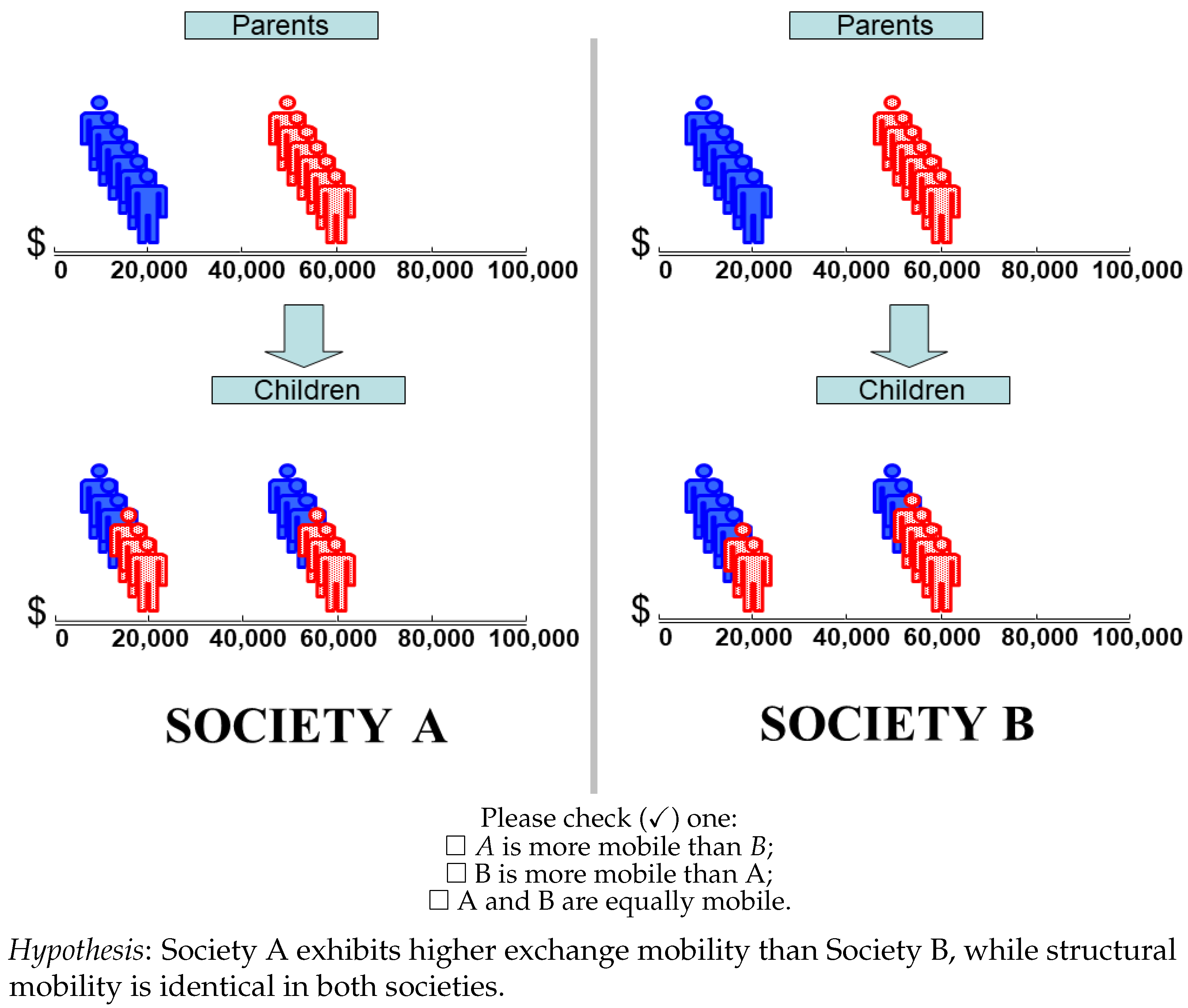
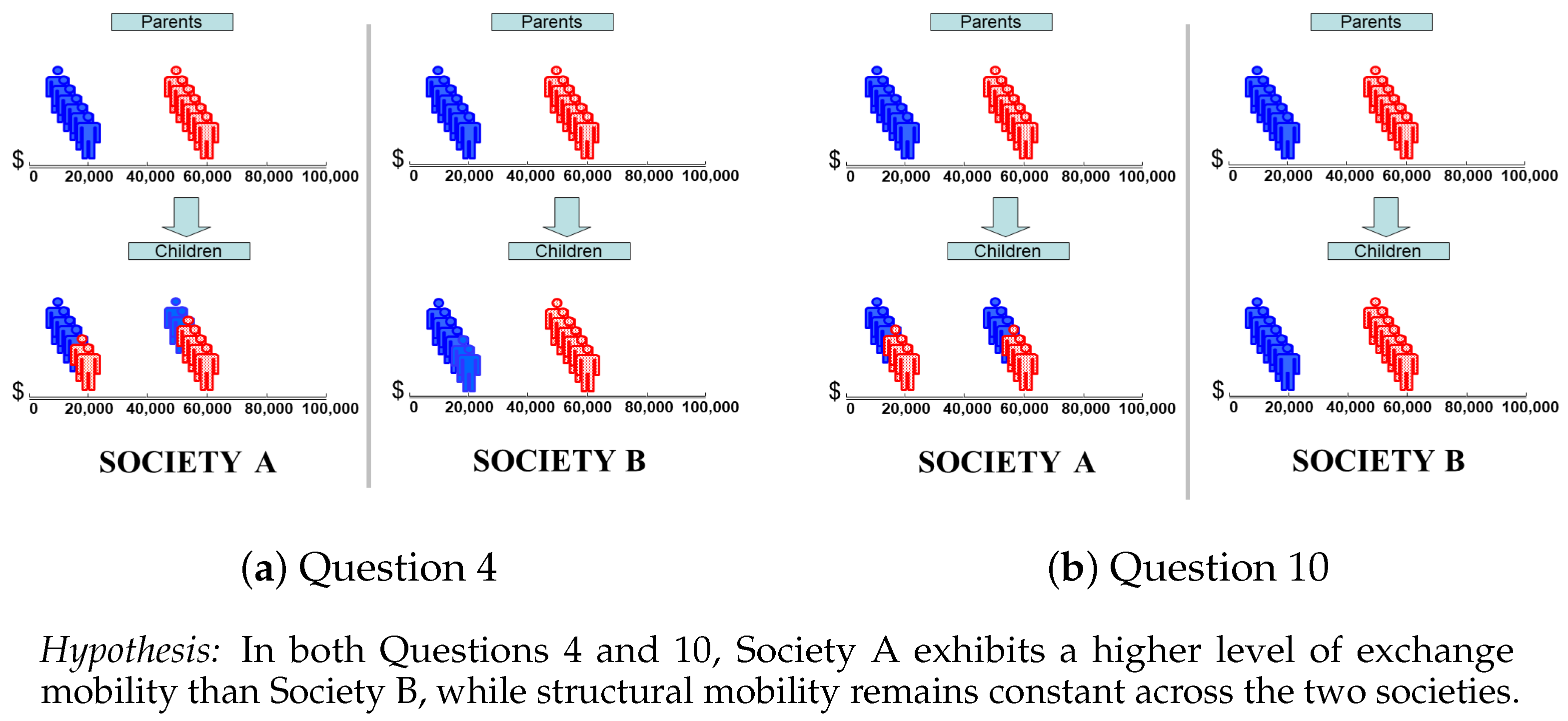
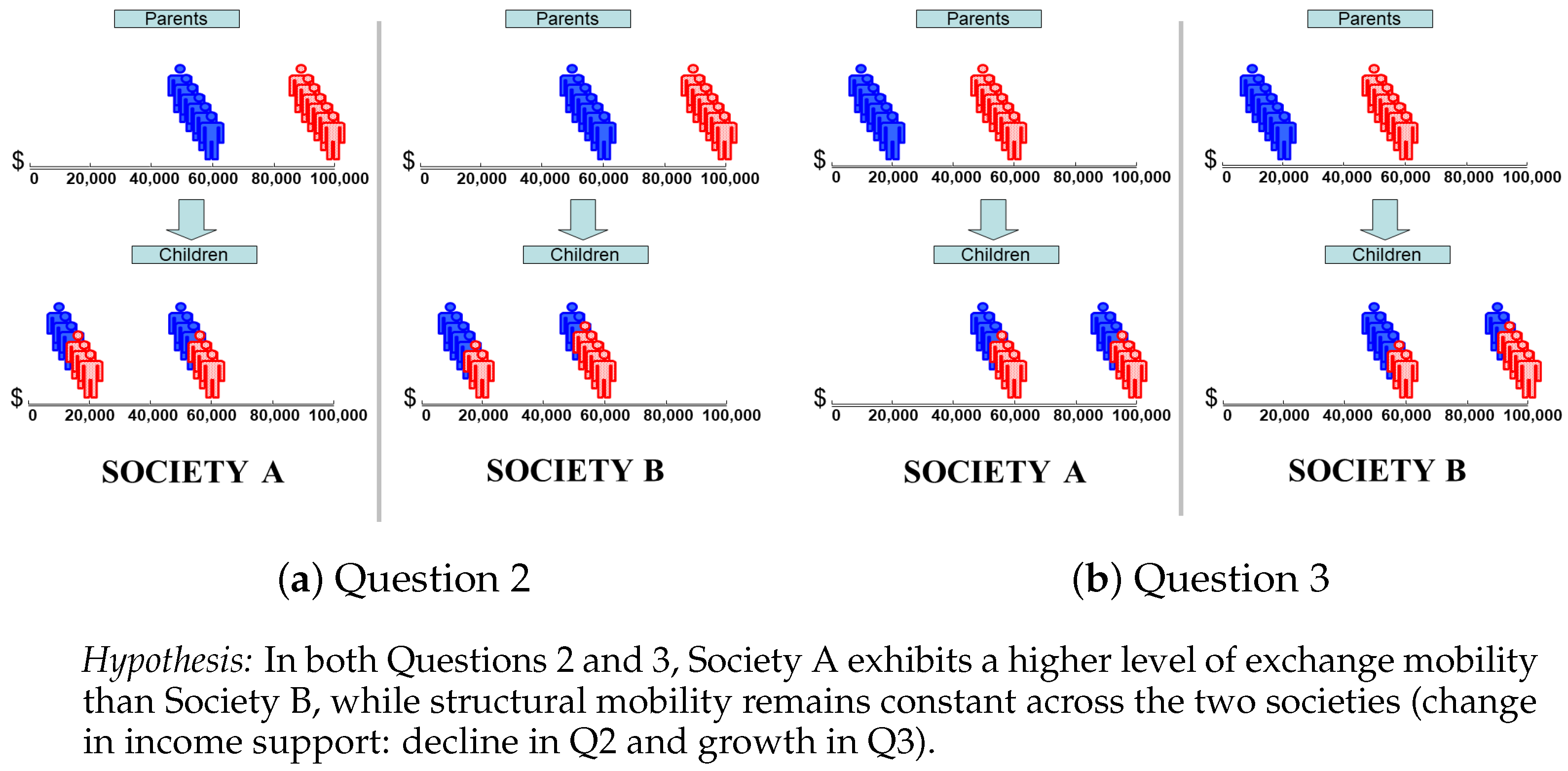
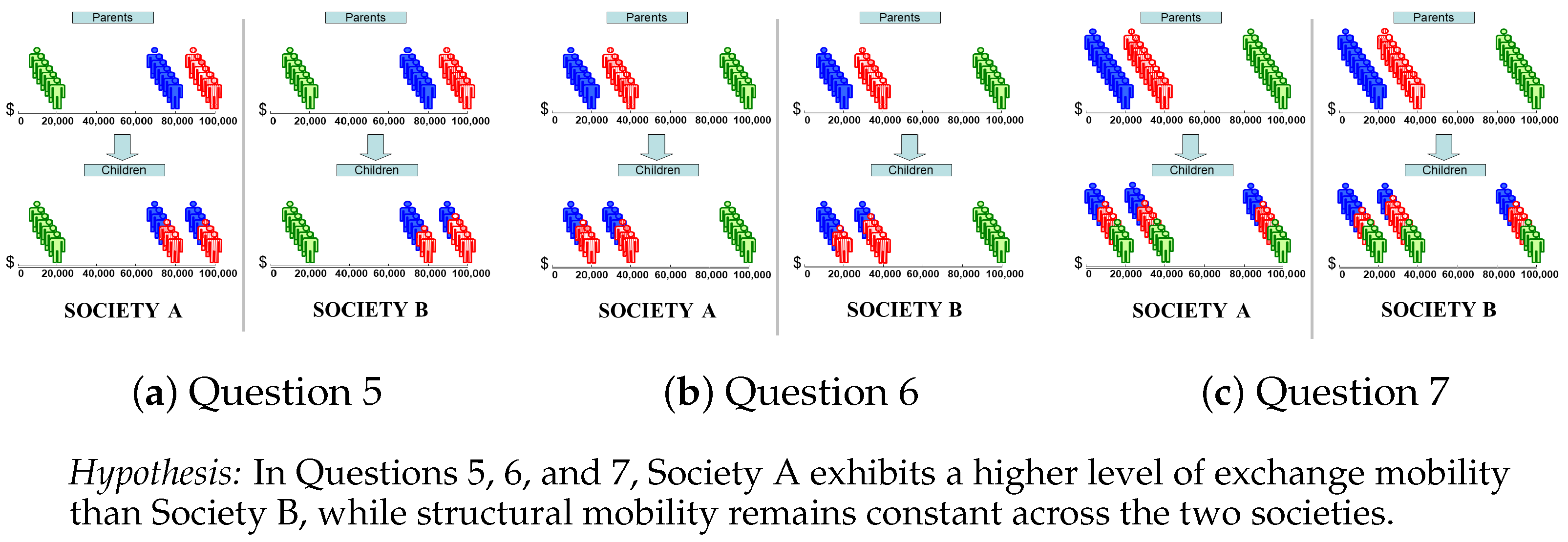
4
In the example below, we adopt this representation for simplicity, where Society A always displays greater mobility. However, in the experimental questionnaire, we randomize both the order of the questions and which society exhibits greater mobility in each question.
5
People who are repeatedly flagged for lack of attention and care in answering questionnaires (incomplete surveys, failure on control questions, or responding too quickly) may be removed from the subject pool.
6
We present the aggregate sample, as we did not find statistically significant differences between respondents assigned to the two questionnaire versions.
7
Nevertheless, some argue that a relatively well-educated sample could be useful for abstract questions that require reasoned judgments, such as assessing whether people’s perceptions are consistent with theoretical predictions (Amiel & Cowell, 1992; Gaertner & Schokkaert, 2012).

References

  1. Acemoglu, D., Egorov, G., & Sonin, K. (2018). Social mobility and stability of democracy: Reevaluating de Tocqueville. The Quarterly Journal of Economics, 133, 1041–1105. [Google Scholar] [CrossRef]
  2. Acemoglu, D., Egorov, G., & Sonin, K. (2021). Chapter 13—Institutional change and institutional persistence. In A. Bisin, & G. Federico (Eds.), The handbook of historical economics (pp. 365–389). Academic Press. [Google Scholar] [CrossRef]
  3. Aguinis, H., Villamor, I., & Ramani, R. S. (2021). MTurk research: Review and recommendations. Journal of Management, 47, 823–837. [Google Scholar] [CrossRef]
  4. Alesina, A., & La Ferrara, E. (2005). Preferences for redistribution in the land of opportunities. Journal of Public Economics, 89, 897–931. [Google Scholar] [CrossRef]
  5. Alesina, A., Miano, A., & Stantcheva, S. (2020). The polarization of reality. AEA Papers and Proceedings, 110, 324–328. [Google Scholar] [CrossRef]
  6. Amiel, Y. (1999). The measurement of income inequality: The subjective approach. In J. Silber (Ed.), Handbook of income inequality measurement (pp. 227–243). Springer Netherlands. [Google Scholar] [CrossRef]
  7. Amiel, Y., Bernasconi, M., Cowell, F., & Dardanoni, V. (2015). Do we value mobility? Social Choice and Welfare, 44, 231–255. [Google Scholar] [CrossRef]
  8. Amiel, Y., & Cowell, F. A. (1992). Measurement of income inequality: Experimental test by questionnaire. Journal of Public Economics, 47, 3–26. [Google Scholar] [CrossRef]
  9. Atkinson, A. B. (1970). On the measurement of inequality. Journal of Economic Theory, 2, 244–263. [Google Scholar] [CrossRef]
  10. Atkinson, A. B., & Bourguignon, F. (1982). The comparison of multi-dimensioned distributions of economic status. The Review of Economic Studies, 49, 183–201. [Google Scholar] [CrossRef]
  11. Bartolucci, F., Forcina, A., & Dardanoni, V. (2001). Positive quadrant dependence and marginal modeling in two-way tables with ordered margins. Journal of the American Statistical Association, 96, 1497–1505. [Google Scholar] [CrossRef]
  12. Benabou, R., & Ok, E. A. (2001). Social mobility and the demand for redistribution: The POUM hypothesis. The Quarterly Journal of Economics, 116, 447–487. [Google Scholar] [CrossRef]
  13. Berinsky, A. J., Huber, G. A., & Lenz, G. S. (2012). Evaluating online labor markets for experimental research: Amazon.com’s Mechanical Turk. Political Analysis, 20, 351–368. [Google Scholar] [CrossRef]
  14. Binzel, C., & Carvalho, J. P. (2017). Education, social mobility and religious movements: The Islamic revival in Egypt. The Economic Journal, 127, 2553–2580. [Google Scholar] [CrossRef]
  15. Cappelen, A. W., Haaland, I. K., & Tungodden, B. (2018). Beliefs about behavioral responses to taxation. Norwegian School of Economics. [Google Scholar]
  16. Chakravarty, S. R., Dutta, B., & Weymark, J. A. (1985). Ethical indices of income mobility. Social Choice and Welfare, 2, 1–21. [Google Scholar] [CrossRef]
  17. Cinquanta, G. (2020). Three essays on social mobility: Mobility dimensions, welfare evaluation and questionnaires evidence [Ph.D. thesis, University of Ca’ Foscari of Venice]. [Google Scholar]
  18. Corak, M. (2013). Income inequality, equality of opportunity, and intergenerational mobility. Journal of Economic Perspectives, 27, 79–102. [Google Scholar] [CrossRef]
  19. Cowell, F. A., & Flachaire, E. (2018). Measuring mobility. Quantitative Economics, 9, 865–901. [Google Scholar] [CrossRef]
  20. D’Agostino, M., & Dardanoni, V. (2009). The measurement of rank mobility. Journal of Economic Theory, 144, 1783–1803. [Google Scholar] [CrossRef]
  21. Dardanoni, V. (1993). Measuring social mobility. Journal of Economic Theory, 61, 372–394. [Google Scholar] [CrossRef]
  22. Dardanoni, V. (1995). Income distribution dynamics: Monotone Markov chains make light work. Social Choice and Welfare, 12, 181–192. [Google Scholar] [CrossRef]
  23. Dardanoni, V., Fiorini, M., & Forcina, A. (2012). Stochastic monotonicity in intergenerational mobility tables. Journal of Applied Econometrics, 27, 85–107. [Google Scholar] [CrossRef]
  24. Dasgupta, P., Sen, A., & Starrett, D. (1973). Notes on the measurement of inequality. Journal of Economic Theory, 6, 180–187. [Google Scholar] [CrossRef]
  25. Davidai, S. (2018). Why do Americans believe in economic mobility? Economic inequality, external attributions of wealth and poverty, and the belief in economic mobility. Journal of Experimental Social Psychology, 79, 138–148. [Google Scholar] [CrossRef]
  26. Davidai, S., & Gilovich, T. (2015). Building a more mobile America—One income quintile at a time. Perspectives on Psychological Science, 10, 60–71. [Google Scholar] [CrossRef]
  27. Day, M. V., & Fiske, S. T. (2017). Movin’on up? How perceptions of social mobility affect our willingness to defend the system. Social Psychological and Personality Science, 8, 267–274. [Google Scholar] [CrossRef]
  28. Decancq, K., Fleurbaey, M., & Schokkaert, E. (2015). Chapter 2—Inequality, income, and well-being. In A. B. Atkinson, & F. Bourguignon (Eds.), Handbook of income distribution (Vol. 2, pp. 67–140). Elsevier. [Google Scholar] [CrossRef]
  29. Fehr, D., & Vollmann, M. (2022). Misperceiving economic success: Experimental evidence on meritocratic beliefs and inequality acceptance. CESifo Working Paper No. 9983. CESifo. [Google Scholar] [CrossRef]
  30. Fields, G. S. (2019). Concepts of social mobility. WIDER Working Paper No. 106. WIDER. [Google Scholar] [CrossRef]
  31. Fields, G. S., & Ok, E. A. (1996). The meaning and measurement of income mobility. Journal of Economic Theory, 71, 349–377. [Google Scholar] [CrossRef]
  32. Fisman, R., Gladstone, K., Kuziemko, I., & Naidu, S. (2017). Do Americans want to tax capital? Evidence from online surveys. NBER working paper series No. 23907. National Bureau of Economic Research. [Google Scholar] [CrossRef]
  33. Fisman, R., Kuziemko, I., & Vannutelli, S. (2021). Distributional preferences in larger groups: Keeping up with the Joneses and keeping track of the tails. Journal of the European Economic Association, 19, 1407–1438. [Google Scholar] [CrossRef]
  34. Fréchet, M. (1951). Sur les tableaux de corrélation dont les marges sont données. Ann. Univ. Lyon 3ˆ e serie Sciences Sect. A, 14, 53–77. [Google Scholar]
  35. Gaertner, W., & Schokkaert, E. (2012). Empirical social choice: Questionnaire-experimental studies on distributive justice. Cambridge University Press. [Google Scholar] [CrossRef]
  36. Gottschalk, P., & Spolaore, E. (2002). On the evaluation of economic mobility. The Review of Economic Studies, 69, 191–208. [Google Scholar] [CrossRef]
  37. Jäntti, M., & Jenkins, S. P. (2015). Chapter 10—Income mobility. In A. B. Atkinson, & F. Bourguignon (Eds.), Handbook of income distribution (Vol. 2, pp. 807–935). Elsevier. [Google Scholar] [CrossRef]
  38. Kolm, S. C. (1976). Unequal inequalities. II. Journal of Economic Theory, 13, 82–111. [Google Scholar] [CrossRef]
  39. Kuziemko, I., Norton, M. I., Saez, E., & Stantcheva, S. (2015). How elastic are preferences for redistribution? Evidence from randomized survey experiments. American Economic Review, 105, 1478–1508. [Google Scholar] [CrossRef]
  40. Markandya, A. (1984). The welfare measurement of changes in economic mobility. Economica, 51, 457–471. [Google Scholar] [CrossRef]
  41. Mengel, F., & Weidenholzer, E. (2023). Preferences for redistribution. Journal of Economic Surveys, 37, 1660–1677. [Google Scholar] [CrossRef]
  42. Paolacci, G., Chandler, J., & Ipeirotis, P. G. (2010). Running experiments on Amazon Mechanical Turk. Judgment and Decision Making, 5, 411–419. [Google Scholar] [CrossRef]
  43. Ray, D., & Genicot, G. (2023). Measuring upward mobility. American Economic Review, 113, 3044–3089. [Google Scholar] [CrossRef]
  44. Stantcheva, S. (2023). How to run surveys: A guide to creating your own identifying variation and revealing the invisible. Annual Review of Economics, 15, 205–234. [Google Scholar] [CrossRef]
  45. Uchida, Y. (2018). Education, social mobility, and the mismatch of talents. Economic Theory, 65, 575–607. [Google Scholar] [CrossRef]
  46. Van de gaer, D., & Palmisano, F. (2021). Growth, mobility and social progress. Journal of Comparative Economics, 49, 164–182. [Google Scholar] [CrossRef]
  47. Van de gaer, D., Schokkaert, E., & Martinez, M. (2001). Three meanings of intergenerational mobility. Economica, 68, 519–538. [Google Scholar] [CrossRef]
  48. Weinzierl, M. (2017). Popular acceptance of inequality due to innate brute luck and support for classical benefit-based taxation. Journal of Public Economics, 155, 54–63. [Google Scholar] [CrossRef]
Figure 1. Example of a question (Question 1).
Games 16 00024 g001
Figure 2. Comparisons with extreme scenario.
Games 16 00024 g002
Figure 3. Comparisons with income changes.
Games 16 00024 g003
Figure 4. Comparisons with three social classes.
Games 16 00024 g004
Figure 5. Comparisons with changes in dynasties’ size and income.
Games 16 00024 g005
Figure 6. Questionnaire results.
Games 16 00024 g006
Table 1. Example of mobility table.
Society A
Parent
Status
Child Status
LowHigh A C
Lowa c L a c L
High p L a 1 p L c L + a 1 c L
A P p L 1 p L
Table 2. Example of mobility tables under comparison.
Society A
Parent
Status
Child Status
LowHigh A C
Lowa c L a c L
High p L a 1 p L c L + a 1 c L
A P p L 1 p L
Society B
Parent
Status
Child Status
LowHigh B C
Lowb c L b c L
High p L b 1 p L c L + b 1 c L
B P p L 1 p L
Table 3. Cumulative joint distribution of societies in Question 5.
Society A
Parent
Status
Child Status
20,00080,000100,000
20,000 1 3 1 3 1 3
80,000 1 3 1 2 2 3
100,000 1 3 2 3 1
Society B
Parent
Status
Child Status
20,00080,000100,000
20,000 1 3 1 3 1 3
80,000 1 3 5 9 2 3
100,000 1 3 2 3 1
Table 4. Sample characteristics.
MeanStandard
Deviation
MinMaxN
(1) (2) (3) (4) (5)
   Demographics—(D)
Age35.2910.621973242
Gender (1 = female, 0 = male)0.380.4901242
Ethnicity (1 = white, 0 = otherwise)0.720.4501242
Education (1 = master’s degree, 0 = less)0.120.3301242
Marital status (1 = married or domestic partnership, 0 = otherwise)0.420.4901242
   Economic prospects—(P)
(P1) Standard of living vs. US average2.710.7515242
(1 = much lower, …, 5 = much higher)
(P2) Standard of living vs. parents2.860.9615242
(1 = much lower, …, 5 = much higher)
(P3) Income opportunities vs. parents3.001.0315242
(1 = much lower, …, 5 = much higher)
   Values—(V)
(V1) Value of independence in economic positions3.770.7415242
(1 = strongly disagree, …, 5 = strongly agree)
(V2) Independence as equality of opportunity3.750.8315242
(1 = strongly disagree, …, 5 = strongly agree)
Table 5. Distributions of answers in (Q1, Q4), (Q1, Q10) and (Q4, Q10).
Q4 Q10
A B = A B =
Q1A48.82%4.72%1.57%Q1A44.88%6.30%3.94%
B15.75%3.15%3.94%B11.81%7.87%3.15%
=10.24%4.72%7.09%=11.81%5.51%4.72%
Q4A62.60%8.66%3.94%
B3.15%8.66%0.79%
=3.15%2.36%7.09%
Note: Results for each of these questions are illustrated in Figure 6a.
Table 6. Distributions of answers in (Q1bis, Q4bis), (Q1bis, Q10bis), and (Q4bis, Q10bis).
Q4bis Q10bis
A B = A B =
Q1bisA54.78%2.61%4.35%Q1bisA55.65%3.48%2.61%
B7.83%8.70%6.09%B7.83%13.04%1.74%
=5.22%4.35%6.09%=6.96%3.48%5.22%
Q4bisA59.13%6.96%1.74%
B3.48%7.83%4.35%
=7.83%5.22%3.48%
Note: Results for each of these questions are illustrated in Figure 6b.
Table 7. Distributions of answers in (Q5, Q6), (Q5, Q6), and (Q6, Q7).
Q6 Q7
A B = A B =
Q5A40.94%5.51%3.94%Q5A28.35%7.09%14.96%
B9.45%16.54%3.94%B9.45%14.96%5.51%
=1.57%4.72%13.39%=5.51%3.94%10.24%
Q6A28.35%8.66%14.96%
B9.45%12.60%4.72%
=5.51%4.72%11.02%
Note: Results for each of these questions are illustrated in Figure 6a.
Table 8. Distributions of answers in (Q5bis, Q6bis), (Q5bis, Q6bis), and (Q6bis, Q7bis).
Q6bis Q7bis
A B = A B =
Q5bisA53.04%4.35%3.48%Q5bisA38.26%10.43%12.17%
B9.57%11.30%1.74%B4.35%14.78%3.48%
=3.48%2.61%10.43%=5.22%1.74%9.57%
Q6bisA38.26%14.78%13.04%
B4.35%9.57%4.35%
=5.22%2.61%7.83%
Note: Results for each of these questions are illustrated in Figure 6b.
Table 9. Distributions of answers in (Q2, Q3) and (Q8, Q9).
Q3 Q9
A B = A B =
Q2A24.41%10.24%3.94%Q8A29.92%23.62%5.51%
B11.81%19.69%4.72%B5.51%18.11%6.30%
=5.51%7.87%11.81%=1.57%3.15%6.30%
Note: Results for each of these questions are illustrated in Figure 6a.
Table 10. Distributions of answers in (Q2bis, Q3bis) and (Q8bis, Q9bis).
Q3bis Q9bis
A B = A B =
Q2bisA27.83%7.83%4.35%Q8bisA34.78%19.13%7.83%
B8.70%24.35%7.83%B3.48%16.52%3.48%
=6.09%6.09%6.96%=2.61%2.61%9.57%
Note: Results for each of these questions are illustrated in Figure 6b.
Table 11. Multinomial logit for questionnaire answers.
Greater Mobility inTest
Society A Society B [ A i ] [ B i ] = 0
(1) (2) (3)
Q1 (2 × 2—stochastic independence)1.076 ***−0.2071.283 ***
(0.287)(0.333)(0.283)
Q2 (as Q1 with income decline)0.562 *0.1210.440
(0.297)(0.315)(0.272)
Q3 (as Q1 with income growth )0.858 ***0.3780.480 *
(0.307)(0.325)(0.267)
Q4 (2 × 2—immobility)1.978 ***−0.2332.211 ***
(0.329)(0.416)(0.330)
Q5 (3 × 3—mobility between middle-top classes)1.097 ***0.1820.915 ***
(0.300)(0.341)(0.274)
Q6 (3 × 3—mobility between bottom-middle classes)      1.050 ***−0.0091.059 ***
(0.294)(0.339)(0.282)
Q7 (3 × 3—mobility between all classes)0.478 *−0.4190.897 ***
(0.288)(0.324)(0.281)
Q8 (2 × 2—changes generations’ size)1.857 ***0.773 **1.084 ***
(0.338)(0.376)(0.272)
Q9 (as Q8 with income growth)0.857 ***0.678 **0.179
(0.320)(0.327)(0.266)
Q10 (2 × 2—immobility)1.948 ***0.2811.666 ***
(0.336)(0.394)(0.286)
Q1bis (2 × 2—stochastic independence)1.492 ***0.0931.399 ***
(0.326)(0.373)(0.291)
Q2bis (as Q1 with income decline)0.822 **0.4800.342
(0.322)(0.332)(0.274)
Q3bis (as Q1 with income growth )0.888 ***0.4140.474 *
(0.325)(0.339)(0.275)
Q4bis (2 × 2—immobility)1.538 ***−0.3321.870 ***
(0.319)(0.396)(0.320)
Q5bis (3 × 3—mobility between middle-top classes)1.421 ***0.0371.384 ***
(0.323)(0.371)(0.291)
Q6bis (3 × 3—mobility between bottom-middle classes)1.566 ***−0.1221.687 ***
(0.324)(0.385)(0.306)
Q7bis (3 × 3—mobility between all classes)0.724 **−0.2250.949 ***
(0.307)(0.338)(0.285)
Q8bis (2 × 2—changes generations’ size)1.550 ***0.1891.361 ***
(0.330)(0.378)(0.298)
Q9bis (as Q8 with income growth)0.754 **0.3240.431
(0.313)(0.331)(0.278)
Q10bis (2 × 2—immobility)2.140 ***0.4741.666 ***
(0.385)(0.431)(0.303)
Age−0.007−0.005−0.002
(0.005)(0.006)(0.005)
Gender (1 = female)0.0940.202−0.108
(0.129)(0.139)(0.107)
Ethnicity (1 = white)0.420 ***0.451 ***−0.031
(0.138)(0.150)(0.120)
Education (1 = master degree)0.672 ***0.700 ***−0.028
(0.216)(0.229)(0.149)
Marital status (1 = married)−0.622 ***−0.047−0.574 ***
(0.127)(0.136)(0.106)
(P1) Standard of living relative to average in the US−0.1190.008−0.126 **
(0.074)(0.079)(0.060)
(P2) Standard of living relative to parents0.227 ***0.246 ***−0.019
(0.084)(0.092)(0.074)
(P3) Income opportunities relative to parents                   −0.053−0.0570.003
(0.079)(0.085)(0.067)
(V1) Independence preferable0.0590.097−0.038
(0.076)(0.081)(0.063)
(V2) Independence as equality of opportunity0.260 ***0.1120.148 **
(0.072)(0.073)(0.062)
Observations2420
Note: The dependent variable takes the value 1 (−1) when the answer is Society A (B), or 0 otherwise. Robust standard error in brackets. Stars *, **, ***, denote rejection at 10, 5, and 1% levels. Controls for economic prospects (P) and values (V) are standardized.
Disclaimer/Publisher’s Note: The statements, opinions and data contained in all publications are solely those of the individual author(s) and contributor(s) and not of MDPI and/or the editor(s). MDPI and/or the editor(s) disclaim responsibility for any injury to people or property resulting from any ideas, methods, instructions or products referred to in the content.

