Article

Sharing Price Announcements

by
Maarten Janssen
1 and
Vladimir Karamychev
2,*
1
Department of Economics, University of Vienna, 1010 Wien, Austria
2
Department of Economics, Erasmus School of Economics, 3062 PA Rotterdam, The Netherlands
*
Author to whom correspondence should be addressed.
Games 2025, 16(2), 13; https://doi.org/10.3390/g16020013
Submission received: 17 December 2024 / Revised: 8 February 2025 / Accepted: 21 February 2025 / Published: 10 March 2025

Abstract

:
We present a simple model where, before competing in prices, firms announce which prices they intend to choose. Deviating from these announcements involves a cost. We show that sharing pricing intentions results in prices being set above their competitive levels. All equilibria result in prices that are higher than in the absence of announcements. When the deviation cost of not sticking to the price announcement is high, the unique equilibrium market outcome is asymmetric, as with price leadership. When this cost is low, a symmetric equilibrium exists with even higher prices. Product differentiation is a key ingredient to these results.
JEL Classification:
D440; L960

1. Introduction

In many cartel cases, firms are accused of sharing price information. Markets that have been investigated and where market players were fined include the market for elevators and escalators,1 trucks,2 and bicycles.3 Even though competition authorities typically have been able to fine the firms involved in sharing price information, the private lawsuits that follow, where buyers try to claim damages for the higher prices they have paid, are typically plagued by long discussions about the theory of harm. One of the relevant issues is that because the sharing of price intentions is unlawful by the per se rule in the United States (under Section 1 of the Sherman Act) and by object in the European Union (under Article 101), competition authorities typically do not have to argue whether or not the cartel inflicted harm on its customers: it suffices to establish that the firms involved shared information about the price they intended to charge without having to establish beyond reasonable doubt the effects of information sharing.
The markets mentioned above are all characterized by high degrees of product differentiation, where the final product is often tailor-made for a particular customer. The price information that is shared is often, however, at a much higher level of abstraction and involves some form of list prices or an intention to raise average prices by a certain level, while no agreements are made on “individual transaction” prices. When the actual transaction prices are not exchanged or discussed, and when the market shares are also not stable over time, with some competitors seemingly gaining market share and others losing market share, the question is what the role of sharing list prices or the sharing of price intentions really is on market outcomes.
Typically, to shed some light on the issue, the collusion literature that builds on the theory of repeated games is used. That literature (summarized in textbooks such as Cabral, 2000; Church & Ware, 2000) gives some conditions under which collusion is more likely to have an effect. Standard results say that if (i) firms have similar (and stable) market shares, (ii) products are more or less homogeneous, and/or (iii) there is a relatively high frequency of interaction between the firms, then collusion is more likely to be successful.4 In addition, for firms to be able to retaliate, prices should be publicly observed so that competitors can check whether other firms stick to the prices they promised. However, in most markets where information is shared, (i) firms are often asymmetric in size and/or in market shares (so that the symmetry condition fails), (ii) firms sell many varieties of their products (so that the products are clearly not homogeneous), and (iii) one may also question whether yearly interactions are frequent enough to allow for trigger strategies to be effective. As individual transaction prices are often not publicly observable, it is also difficult to see how competitors can retaliate if some firm deviates. Does this imply that the sharing of prices or price intentions is (likely) not harmful in these markets, or at least that economic theory does not provide a basis for claiming that harm is likely in these markets?
This paper builds a simple model that helps evaluate the implications of price announcements. We explicitly model announcements of price intentions (or the setting of list prices indicating the direction in which prices should develop) and pricing decisions as separate (and sequential) choices in a heterogeneous product market. Firms can choose to be deliberately vague about their future prices by announcing a very wide interval of prices. To potentially have an effect, it should be costly for firms to set prices that differ from their (possibly vague) price intentions. We are agnostic about what this cost could be. For example, it could be a reputation cost, namely that competitors will not believe a firm’s price announcements in the future if it deviates from the current price announcement. Alternatively, the cost of deviating from the price announcement can be motivated from a principal-agent perspective, where the principal within a firm (say central management) sets price intentions, communicates them to other firms, and imposes costs for (sales) agents if they deviate from the announcement. In both interpretations, no costs are incurred if the set price is consistent with the (interval of) the announced prices.
In the main part of the analysis, we assume that the cost of deviation is linear in the size of the deviation and is symmetric in deviations upwards and downwards. Within this simple modeling environment, we have three results. First, for any cost of deviating, equilibrium transaction prices are always larger than the competitive price, which would have resulted in the absence of price announcements. The argument is in two steps. First, announcing a potentially binding upper bound on one’s price is weakly dominated by not announcing such an upper bound. Under product differentiation, firms’ prices are strategic complements. In this case, announcing an upper bound restricts the prices the firm can set and, therefore, has the potential strategic effect that a competitor will also not set high prices. Because both effects can only reduce profits, announcing an upper bound is clearly not in the interest of a firm. Second, firms individually then have an incentive to impose a lower bound on their price that is (at least) marginally larger than the non-cooperative equilibrium price. This is so because the second-order negative effect on their own profit is outweighed by a first-order positive indirect effect on their profits through the (positive) price reaction of their competitor.
We next inquire into the results when the cost of deviating from the price intentions is so large that no firm will ever want to deviate from the announcement. Thus, the announcement gives the firm full commitment power. We show that the unique subgame perfect equilibrium market outcome is asymmetric: one firm announces a lower bound on the prices it will set that is equal to the price a Stackelberg Leader will choose in a pricing game with product differentiation. The other firm will choose the price that is the best response to it. Both firms are better off than without price announcements, but the firm that best responds and acts like a Stackelberg Follower benefits the most. Interestingly, even though firms are ex ante identical, symmetric equilibria in pure strategies do not exist.5 This is so because both equilibrium announcements must be above the competitive equilibrium price and, therefore, be restrictive. However, if the rival is restricted, it is optimal to choose to best respond and not be restricted.
Product differentiation is crucial to the result. In the extreme case of heterogeneous product markets where firms are local monopolists, announcing prices to affect other firms’ prices makes no sense. When firms’ products are getting more homogeneous, two effects appear. First, the competition intensity increases. As a result, firms’ prices and profits without price announcements decline and approach the Bertrand limiting case when the products become perfectly homogeneous. Second, the effect of price announcements becomes stronger, and the firms’ prices and profits increase relative to the Bertrand outcome. The interaction of these two effects results in equilibrium prices and profits being highest when there is a moderate degree of product differentiation. When firms’ products are completely identical, the second effect is not present, and no binding announcements are made in equilibrium.
Our final set of results pertains to environments where the cost of not sticking to the announced prices is small. If deviating from the price announcement involves a cost, the announcement provides only partial commitment power. Then, first, asymmetric equilibria, which are similar to those with full commitment power, always exist. In these equilibria, the price that is announced is such that knowing that the rival will best respond, the announcing firm does not want to deviate to the best response to the rival’s choice. Second, if the cost of deviating from the announcement is small enough, then also a symmetric equilibrium exists where both firms announce a binding lower bound on the price they intend to charge. The equilibrium price is increasing in the cost of deviating. At a certain cost level, the symmetric equilibrium disappears. Importantly, for the same costs, symmetric equilibrium prices are always higher than prices in asymmetric equilibria.
We then analyze the model when the cost of deviating from the announcement is a fixed cost that is independent of the size of deviations. Fixed deviational costs result in discontinuous firms’ best responses in price competition subgames and a multiplicity of Nash equilibria in these subgames. We focus on equilibria where firms’ price announcements have a monotone effect on their pricing strategy, whenever possible. Using this equilibrium selection criterion, we show that all results we obtain for linear costs of deviations continue to hold. Moreover, we show that even if the cost of not sticking to the announced prices is small, the market outcome can be significantly different from the non-cooperative equilibrium, although in the limit, when the cost approaches zero, the market outcome converges to the non-cooperative outcome. We illustrate all our results with a numerical example widely used in the IO literature, where firms’ market demands are linear, and production costs are zero.
To emphasize the importance of these results for actual competition cases, a few comments are in order. First, rather than being an obstacle to achieving collusion, product differentiation is key to the results. In a homogeneous product market, a rival always wants to undercut the price announcement, and no announcement will be made. Second, in any of the asymmetric equilibria, price announcements can be effective even if there is no clear relationship between the announcements and prices. The reason is that the equilibrium strategies are not unique. Not only does the upper bound of price announcements remain undetermined but also the lower bound price announcement of one of the firms, as long as its best response to the Leader’s announcement is included. Third, unstable market shares do not indicate that the announcements are ineffective. Indeed, the presence of asymmetric equilibria shows that price announcements can be effective even if some firms gain market share relative to others. Finally, transaction prices need not be publicly observed for price announcements to have a collusive effect because the market equilibrium can be sustained without retaliation possibility.
The paper that is closest to ours is Harrington (2022), which also analyses a Bertrand competition model with heterogeneous products, where firms make price announcements in the first stage and choose actual transaction prices in the second stage. Harrington (2022) also introduces the cost of not sticking to the announcement. There are a few modeling differences, however, that result in substantially different outcomes. In Harrington (2022), only symmetric equilibria are considered, the announcements are restricted to a single price, and the cost of deviating from the announcement is asymmetric: it is infinitely high for price increases and linear in the size of deviations for price decreases. These differences lead to two crucial differences in results. First, according to Harrington (2022), an equilibrium where firms announce their competitive prices always exists. As explained above, such an equilibrium does not exist in our setting as firms have an incentive to increase their price announcements: announcing an upper bound is weakly dominated. Second, asymmetric equilibria are an important part of our equilibrium characterization. Where Harrington (2022) establishes that if the cost parameter is small enough, there exists a symmetric equilibrium where firms make price announcements above their competitive levels, we show that additionally asymmetric equilibria always exist so that above competition price levels will persist even if the cost of deviation from the announcement is large. These differences also have practical relevance. First, our theory suggests that price announcements necessarily have anti-competitive effects, whereas, on the basis of Harrington (2022), one can only argue that they could have an anti-competitive effect and only if the cost of deviating is small. Second, one rarely observes firms making identical price announcements. Firms can use this observation to argue against the relevance of Harrington (2022) as, in contrast to ours, that analysis cannot account for asymmetries.
There is also some literature that is less closely connected. In particular, there is literature on two-stage pricing without the cost of adopting different prices. For example, Raskovich (2007) and Gill and Thanassoulis (2016) study how price discrimination with list prices, where some consumers get a discount (that is either random or obtained through bargaining), can affect market outcomes. There is also some literature on recommended prices that are communicated to consumers such that the first-stage prices may guide their search behavior, see Lubensky (2017) and Harrington and Ye (2019). García Díaz et al. (2009) study how list prices may affect market outcomes in the presence of capacity constraints. In our paper, the price announcements need not be known to consumers to have an effect while all consumers pay the same price.
The rest of the paper is organized as follows. Section 2 presents the model, and Section 3 establishes that all equilibria have prices above their competitive levels. Section 4 then considers the case where the cost of deviating from the announcements is large, while Section 5 analyses the case of small costs of deviations. In Section 6, we analyze the model for a fixed cost of deviations from price announcements. Section 7 concludes. Proofs are given in the Appendix A.

2. The Model

Consider a market where two firms, i = 1 , 2 , produce horizontally differentiated products. The firms simultaneously set prices p i and p i , and face (symmetric) individual demands D i = D p i , p i . We assume that D p , p is not increasing in p , and D p , p = 0 for all p p ¯ , for some price p ¯ . In all what follows, we assume p 0 , p ¯ . For simplicity, we consider that the unit production cost c 0 is constant so that firm i ’s profit equals:
π i π p i , p i = p i c D p i , p i .
We introduce the following standard assumptions: firms’ products are substitutes, firms’ pricing strategies are strategic complements, and firms’ profits are concave in their own price. Formally, we assume that:
π p i > 0 , 2 π p i p i > 0 , 2 π p i 2 < 0 .
Under these assumptions, the firms’ best responses B R p as defined by π p i B R p , p = 0 are upward sloping. We also define the generalized best response function B R ~ p , γ by π p i B R ~ p , γ , p = γ for any γ 0 .6 We consider that the pricing game has a unique ‘normal’ Nash equilibrium p i = p i = p N > c that is given by B R p N = p N .7 In this Nash equilibrium, firms’ profits are given by:
π i = π i = π N π p N , p N .
Importantly for the analysis that follows, B R p > p for all p < p N , and B R p < p for all p > p N .
Finally, for any γ 0 , we define a generalized ‘price-leader’ profit function as follows:
π ~ L p , γ   π p , B R ~ p , γ .
We assume that the sequential (Stackelberg) pricing game has a unique subgame perfect Nash equilibrium (SPNE), in which the leader sets price p L defined by π ~ L p p L , 0 = 0 , and the follower sets price p F = B R p L .8 In this SPNE, firms’ profits are given by:
π i = π L π ~ L p L , 0 = π p L , B R p L ,
for the leader, and by:
π i = π F π B R p L , p L ,
for the follower. In numerical examples that follow, we set c = 0 and consider the following linear demand function:
D p i , p i = 1 b p i + d p i p i ,
with b > 0 and d 0 . The parameter d can be interpreted as a measure of product differentiation, where larger values represent more homogeneous markets. In this case, the Nash equilibrium prices p N and profits π N of the normal pricing game are given by:
p N = 1 2 b + d , π N = b + d 2 b + d 2 ,
while the subgame perfect equilibrium outcome of the sequential (Stackelberg) pricing game is given by:
p L = p N + d 2 2 2 b + d 2 d 2 2 b + d , p F = B R p L = p N + d 3 4 b + d 2 b + d 2 d 2 2 b + d .
We consider a two-stage game. In stage one, firms simultaneously announce a price range L i , H i , with 0 L i H i . In stage two, firms choose prices. If in the second stage firm i deviates from its announcement, it incurs cost C :
C p i , L i , H i = γ L i p i , if p i < L i   0 , if p i L i , H i γ p i H i , if p i > H i   ,
which is linear in the size of the deviation.
In Section 4, we consider a case when γ is large. Both firms observe each other’s announcements and play the simultaneous-move price competition game described above with prices p i L i , H i . In Section 5, we consider a case when γ is small. Firms may find it optimal to break their announcements and charge prices p i outside of the interval L i , H i . We solve the game for pure strategy SPNE in weakly undominated strategies where firms announce L i , H i , and set prices according to strategies p i = p i L i , L i , H i , H i .

3. Announcements Lead to Collusive Prices

In this section, we show that independent of the cost of deviating from the announcement, prices must be above their competitive levels in any SPNE where firms choose weakly undominated strategies. In the next section, we show by construction that such equilibria exist.
Our analysis starts with a consideration of how the second stage of the game is played, depending on the announcements made by firms. In addition to the unrestricted best-response function B R p , we denote by R i = R p i , L i , H i the second-stage best-response function of firm i that has announced a price range L i , H i . If firm i were unrestricted in the second stage of the game, it would have set price p i = B R p i . Since the profit function π p i , p i of firm i is concave in p i , it then follows that if the cost of deviating from the announcement is sufficiently high, the second stage best-response price of firm i is given by:
R p , L i , H i = L i , if   B R p < L i   B R p , if   B R p L i , H i H i , if   B R p > H i .
Two equations p i = R p i , L i , H i and p i = R p i , L i , H i determine the unique pricing equilibrium p i , p i for the second stage of the game, where p i L i , L i , H i , H i is weakly increasing in all its arguments.
More generally, if the cost of deviating from the announcement is smaller, the first and last parts of the above expression must be relaxed and replaced by weakly increasing functions. In the following lemma, we describe firms’ best responses R p , L i , H i and Nash equilibria.
Lemma 1. 
For any announcement  L i , H i , the second-stage best-response function  p i = R p i , L i , H i  of firm  i  exists, it is single-valued and continuous. There exist price thresholds  z L ,  y L ,  y H , and  z H ,  z L y L y H z H , such that  R p , L i , H i  is given by:
R p , L i , H i = B R ~ p , γ , if p 0 , z L L i , if p z L , y L B R p , if p y L , y H H i , if p y H , z H B R ~ p , γ , if p z H , p ¯ .
Nash equilibrium  p i , p i  always exists, is unique, and is determined by  p i = R p i , L i , H i . The equilibrium price  p i = p L i , L i , H i , H i  is weakly increasing in all its arguments.
According to this lemma, if firm i ’s best response B R p i belongs to the announced price range L i , H i , firm i charges price R i = B R p i L i , H i . In this case, we say the announcement is not binding, and the firm is unrestricted. Otherwise, the announcement is binding. The firm is either restricted by its announcement and charges the announced upper or lower bound price if R i = L i > B R p i or R i = H i < B R p i , or it charges the deviational best response price B R ~ p i , γ < L i or B R ~ p i , γ > H i and pays the deviational cost C . In the latter case, we say the firm breaks the announcement. This concludes the equilibrium analysis of the second stage.
It follows from Lemma 1 that any first-stage announcement H i that can be binding (so that y H < p ¯ ) is weakly dominated. This is because p i L i , L i , H i , H i is weakly increasing in H i . Announcing a sufficiently high price H i that never binds, e.g., H i = p ¯ , results in a weakly higher p i . This, in turn, results in a weakly higher profit π i since the goods are substitutes. Moreover, when y H < p ¯ , announcing H i = p ¯ results in a strictly higher profit π i when p i > y H . Accordingly, announcing any price H i that could be binding is weakly dominated. As only L i may be binding in an equilibrium in weakly undominated strategies, we simplify the notation and denote the second-period best responses by R i = R p i , L i and equilibrium prices by p i = p L i , L i . An SPNE is, therefore, characterized by equilibrium price announcements L i , L i and second-period prices p i , p i .
Finally, we are in the position to state our first main result, namely that all equilibria result in transaction prices that are larger than the normal competitive price p N .
Proposition 1. 
In any pure strategy SPNE in weakly undominated strategies,  p i > p N .
An essential part of the argument is that in equilibrium, both firms will not choose non-binding announcements L i p N . If this were the case, the second-period equilibrium prices would have been equal to p N , and both firms would have received profit π N . If firm i , however, unilaterally deviates and announces L i = p N + ε , where ε > 0 is a small positive number, this firm becomes restricted in the pricing subgame and sets price p i = L i . As the other firm remains unrestricted, it will set price p i = B R L i so that firm i gets profit π i = π ^ ε , where:
π ^ ε π p N + ε , B R p N + ε .
Note that at ε = 0 : π ^ 0 = π p N , B R p N = π N and π ^ 0 > 0 as:
π ^ 0 = π p i p N , p N · d B R d p p N > 0 ,
so that the deviation is profitable: the direct effect of p i on the profit of firm i is of second-order magnitude, whereas the indirect effect of p i on the profit of firm i via R i   is of first-order magnitude and positive.

4. Full Commitment to Price Announcements

In this and the next section, we construct SPNE to show the features that equilibria with price announcements exhibit. In this section, we restrict ourselves to the cost of deviating from the announcements being so large that no firm would ever want to do so.
In the case of large costs, symmetric equilibria will never exist. Given the analysis of the previous section, the argument is straightforward. In a symmetric equilibrium, had it existed, the price announcement L i of each firm i must be binding so that L i = L i = L > p N and p i = p i = L , and firms get a profit equal to π L , L . Since B R L < L , firm i has an incentive to deviate and make a non-binding announcement, e.g., L i B R L . In the subgame after this deviation, firm i is unrestricted and firm i is restricted by its announcement L . The subgame NE prices are p i , p i = B R L , L . Firm i would have liked to break its announcement L i and to lower its price below L . This, however, is too costly. As a result, the profit of firm i is π B R L , L > π L , L so that the deviation is profitable.
Thus, it should not come as a surprise that despite the firms being ex ante symmetric, the only equilibrium outcome is the one in which firms behave asymmetrically, with one firm announcing a price restriction and the other best responding to it. In equilibrium, one firm acts as a price leader and sets price p L , and the other firm follows by choosing price p F .
Proposition 2. 
There are two cost thresholds  γ ¯ A  and  γ ¯ S ,  0 < γ ¯ A γ ¯ S , such that:
1. 
If γ γ ¯ A , then there is a pure strategy SPNE outcome in weakly undominated strategies. The outcome is asymmetric, with one firm announcing  L i = p L  and the other firm making a non-binding announcement  L i  such that  L i p F , and  π B R L i , L i π L . In the pricing subgame, the firm that has announced  L i = p L  charges price  p i = p L , while the other firm charges price  p i = p F . The SPNE profits are  π i = π L  and  π i = π F .
2. 
If  γ γ ¯ S , this outcome is the unique SPNE outcome.
We draw two important conclusions from this Proposition. First, instead of being a problematic issue of real-world markets, asymmetries are natural outcomes of having firms make price announcements if the cost of deviating from the announcement is large. A pure strategy equilibrium is always such that one firm makes a binding announcement, while the other simply best responds. Second, as the discussion of the linear demand example below also makes clear, product differentiation is crucial to the result. If the firms’ products were homogeneous, then a firm that makes a binding announcement would not have had any demand, breaking the rationale for setting higher announcements.
To see the last point more clearly, we use the linear demand example to illustrate the effect of product heterogeneity by varying the product differentiation parameter d . From the relevant expressions of Section 2, it is clear that if d becomes large, then the prices p N , p L , and p F all converge to zero, and in the limit, there is no effect of the possibility to announce prices in advance.
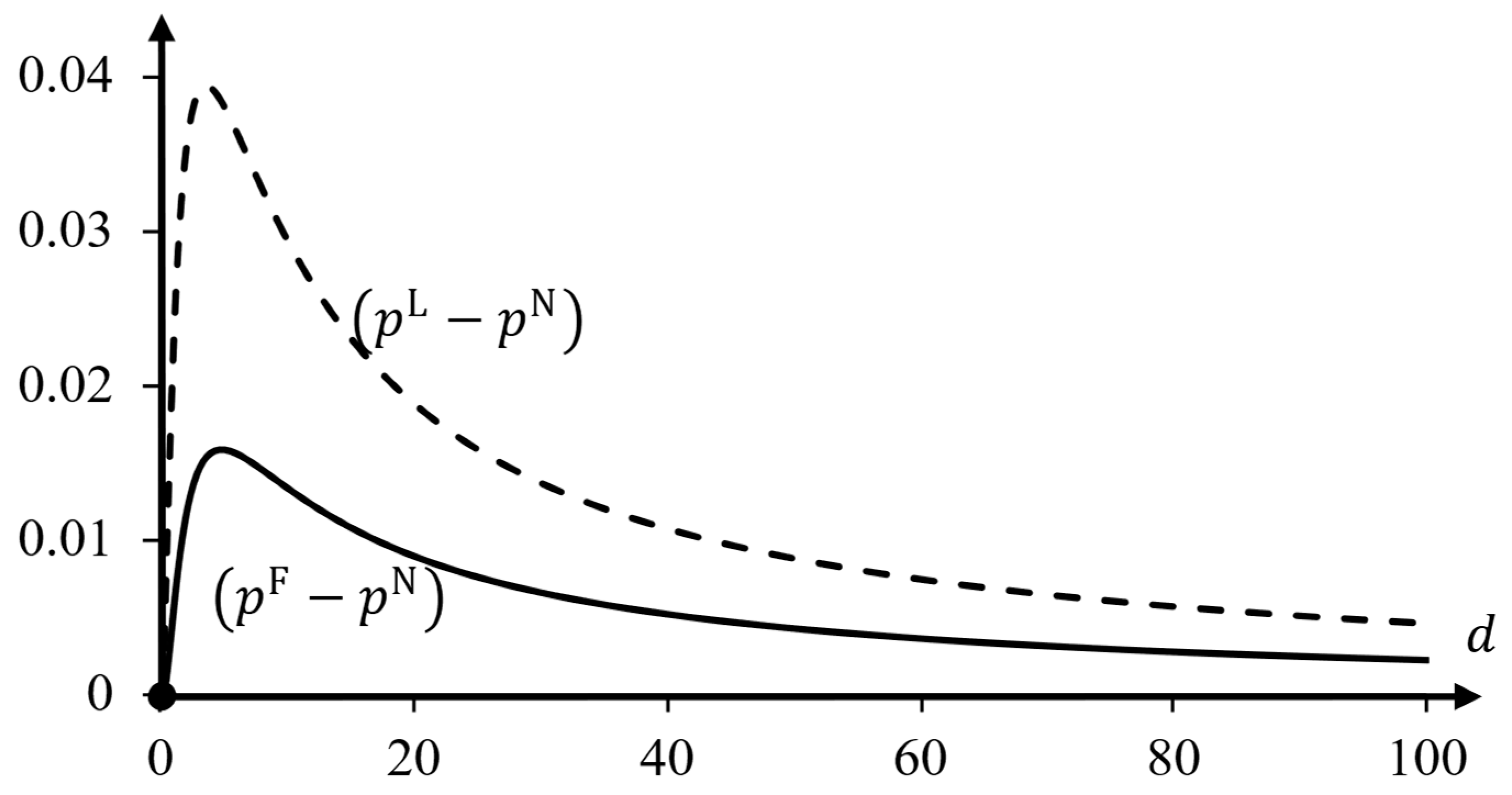
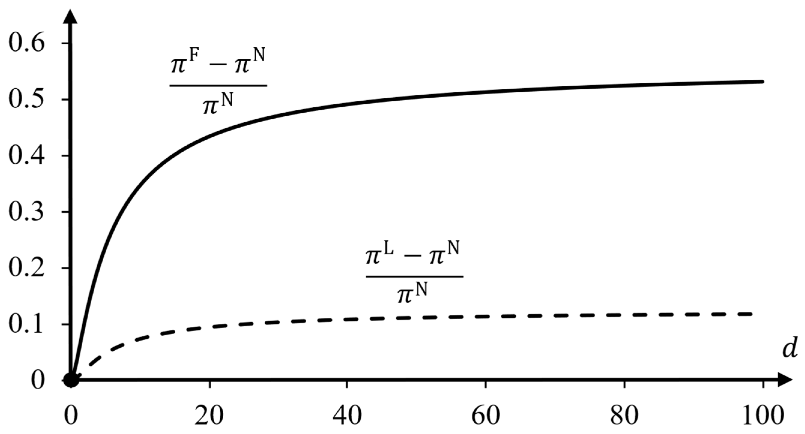
In Figure 1 and Figure 2, one can see that for the linear demand example with b = 1 and c = 0 , the effect of making announcements on absolute levels of market prices is non-monotonic in the degree of product differentiation d (Figure 1), whereas the relative price difference is increasing in the product differentiation parameter, (Figure 2). Interestingly, for intermediate values where the absolute difference is large, prices can go up by as much as 15% and 40%. As the price differences between the two firms lead to opposite effects on their demands, the firm that makes a binding announcement benefits the least, despite its larger price increase. Figure 3 shows that the announcing firm can still make a profit gain of 12.5% when d unboundedly increase, while the other firm’s profit may even increase by 56.25%.

5. Partial Commitment to Price Announcements

In this section, we assume that the marginal cost of deviating from the price announcement γ is small. In this case, the SPNE characterized in Proposition 2 may not anymore be an equilibrium as the price leader will find it optimal to deviate from price p i = p L to price p i = B R p F in the pricing subgame. As announcing L i = p L is not credible anymore, an important question is whether the possibility of making price announcements still has an effect on the equilibrium transaction prices.
The next proposition shows this to be the case and contains three results. First, the asymmetric equilibrium characterized in the previous section naturally transits to smaller costs of deviating from the price announcement. For smaller costs, price announcements naturally lose some of their commitment power. But still, the nature of the equilibrium construction remains the same: only one firm makes a binding announcement, and this firm knows that the other firm will best respond to this announcement. The level of the announcement is now restricted by the fact that it should remain credible.
Second, in addition to the asymmetric equilibria, a symmetric equilibrium may exist, if the cost parameter γ is small enough. In this symmetric equilibrium, both firms make such an announcement that the profit from sticking to it equals the profit from best responding to it, including the deviational cost. Third, prices and profits in the symmetric equilibrium are always higher than those in asymmetric equilibria.
Proposition 3. 
1 
For any γ 0 , γ ¯ A , where  γ ¯ A , is defined in Proposition 2, asymmetric pure strategy equilibria exist. In all such SPNE, one firm  i  announces  L i = p A γ p N , p L  while the other firm  i  remains unrestricted. Firm  i  charges price  p i = p A γ  and the other firm charges price  p i = B R p A γ . Price  p A γ  increases in  γ  and is uniquely determined by equation:
p A = B R ~ B R p A , γ .
2 
There is a cost threshold γ _ S ,  γ _ S γ ¯ S  , where  γ ¯ S  is defined in Proposition 2, such that for any  γ 0 , γ _ S , a symmetric pure strategy equilibrium exists and is unique. In this SPNE, both firms announce  L i = L i = p S γ > p N  and choose prices  p i = p i = p S γ . Price  p S γ  increases with  γ  and is uniquely determined by equation:
p S = B R ~   p S , γ .
3 
For  γ 0 , γ _ S ,  p S γ > p A γ .
When γ increases from zero to γ ¯ A , the asymmetric SPNE announcement is L i = p A γ , and it increases from p N to p L . When γ > γ ¯ A , the asymmetric SPNE announcement is L i = p L . Similarly, p S γ increases with γ . To understand why the symmetric SPNE may not be sustained at high cost levels, note that the equilibrium announcement p S should naturally satisfy π p S , p S π B R p S , p S C . Moreover, this inequality should actually hold as equality because otherwise, firms are restricted, and each firm has an incentive to deviate and marginally lower its announcement. This implies π p S , p S = π B R p S , p S C . If firm i deviates and announces L i < p S , then NE prices are p i , p i = L i , B R ~   L i , γ and firm i gets profit π ~ L L i , γ = π L i , B R ~ L i , γ . Therefore, p S γ is an asymmetric SPNE announcement only if p S γ p ~ L γ , where price p ~ L γ maximizes π ~ L p , γ . If, for some level of γ , p S γ > p ~ L γ , then p S γ is not an SPNE announcement because each firm has a profitable deviation L i = p ~ L γ < p S γ . This issue does not arise in the asymmetric SPNE, in which the rival firm always best responds in the pricing game, and the firm wants to charge the price of a price leader and to be committed to that.
The reason behind the two cost thresholds γ _ S and γ ¯ S is that both p S γ and p ~ L γ increase with γ so that the equilibrium condition p S γ p ~ L γ , which always holds for small γ and always fails for large γ , is impossible to assess for a middle-range values of γ . Thresholds γ _ S and γ ¯ S are defined as the smallest and the largest roots of the equation p S γ = p ~ L γ so that for γ γ _ S , γ ¯ S , p S is the SPNE price announcement if and only if p S p ~ L . In the example that follows, γ _ S = γ ¯ S so that both thresholds coincide. Finally, inequality p S > p A follows immediately from the defining equations.
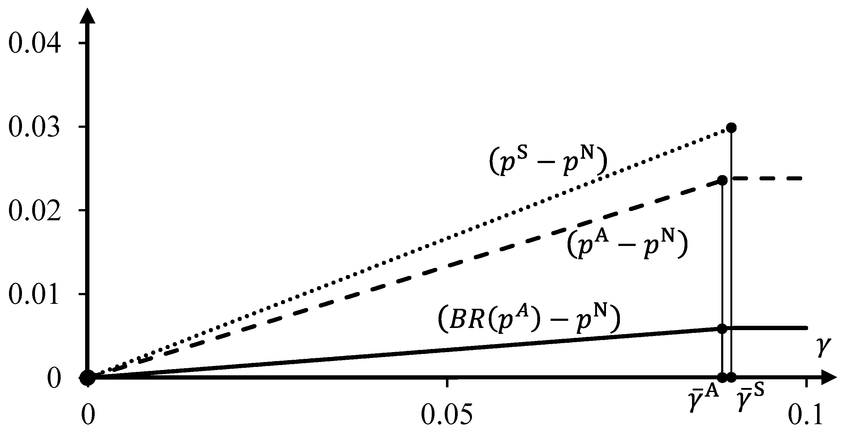
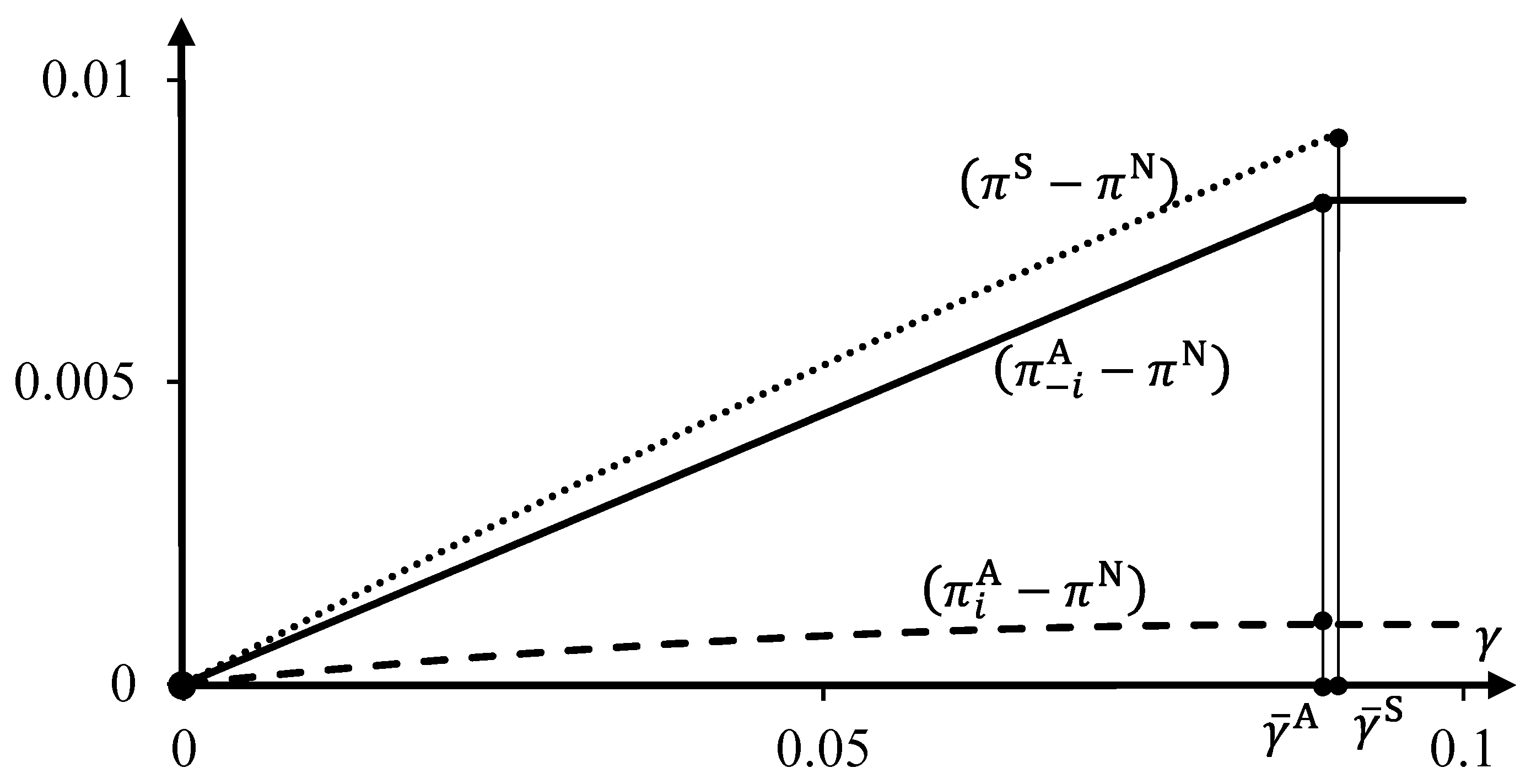
Figure 4 and Figure 5 illustrate the impact of γ on equilibrium prices p A , B R p A , and p S (Figure 4), and profits π i A = π p A , B R p A , π i A = π B R p A , p A , and π S = π p S , p S (Figure 5) for the linear demand example. The parameters c = 0 and b = d = 1 are chosen such that p N = 1 3 , π N = 2 9 . The cost thresholds are given by γ ¯ A = 5 56 and γ _ S = γ ¯ S = 1 11 (at the end of the appendix, we provide expressions for γ ¯ S and γ ¯ A for different parameter values).
The asymmetric equilibrium values are constant for γ γ ¯ A , illustrating Proposition 2. For γ < γ ¯ A , prices and profits are monotonically increasing in γ for the asymmetric equilibrium of Proposition 3. In this example:
p A = 1 3 1 + 4 5 γ , B R p A = 1 3 1 + 1 5 γ π i A = 1 9 1 + 4 5 γ 2 7 5 γ , π i A = 2 9 1 + 1 5 γ 2
When γ < γ ¯ S , prices and profits of the symmetric equilibrium lie above those of the asymmetric equilibrium:
p S = 1 3 1 + γ > p A > B R p A π S = 1 9 1 + γ 2 γ > π i A > π i A .
In both symmetric and asymmetric equilibria, firms benefit from a stronger commitment value, i.e., from a higher value of γ .

6. Fixed Cost of Deviations

When the cost of deviation is independent of the announced and chosen prices, we assume that when firm i deviates from its announcement, it incurs cost C :
C p i , L i , H i = β , if p i L i , H i 0 , if p i L i , H i
Here, β is the fixed cost of a deviation, whatever its size and direction is. It is easy to see that if β is large, all results that we have obtained in Section 4 continue to hold. This is so because if the price announcement is binding, it does not matter how exactly the cost of deviation is determined: it is sufficient it is high enough. When β is small, a new phenomenon arises in pricing subgames: the possibility of equilibrium multiplicity.
Lemma 2. 
For any announcement   L i , H i , the second-stage best-response function  p i = R p i , L i , H i  of firm  i  exists, it is multi-valued and not continuous. There exist price thresholds  z L ,  y L ,  y H , and  z H ,  z L y L y H z H , such that  R p , L i , H i  is given by:
R p , L i , H i = B R p , if p i 0 , z L y L , y H z H , p ¯ B R p , L i , if p i = z L L i , if p i z L , y L H i , if p i y H , z H B R p , H i , if p i = z H
Best response  R p , L i , H i  is discontinuous and double-valued and at  p z L , z H . Nash equilibrium  p i , p i  always exists, is not necessarily unique, and is determined by conditions  p i = R p i , L i , H i .
We use the same terminology as in Section 3 and say that if B R p i L i , H i , then firm i is unrestricted, and its announcement is non-binding. In this case, R i = B R p i L i , H i . Otherwise, the announcement is binding. The firm is either restricted by the announcement and charges the announced upper or lower bound price if R i = L i > B R p i or R i = H i < B R p i , or it charges the deviational best response price B R p i L i , H i and pays the deviational cost C = β . In the latter case, we say the firm breaks the announcement.
The possibility of equilibrium multiplicity in pricing subgames implies that there are multiple reduced-form games. Moreover, Nash equilibrium prices p i = p L i , L i , H i , H i are not necessarily continuous in announcements L i , L i , H i , H i . E.g., announcement L i might affect which Nash equilibrium in prices is played even though L i is not binding. To discard this type of equilibria that are based on such implausible strategies, we impose the following equilibrium selection requirements.
Equilibrium Selection Requirements. 
Let the announcements  L i 0 , L i 0 , H i 0 , H i 0  result in NE  p i 0 , p i 0  of the subgame. Suppose firm  i  lowers its lower-bound  L i 0  by announcing  L i 1 < L i 0 , and this results in NE  p i 1 , p i 1  of the subgame  L i 1 , L i 0 , H i 0 , H i 0 . Then:
1. 
If  L i 0  is not binding, neither is  L i 1 , and NE prices remain the same. Formally, if  L i 1 < L i 0 p i 0 = B R p i 0  then  p i 1 , p i 1 = p i 0 , p i 0 .
2. 
If firm  i  is restricted by  L i 0  in NE  p i 0 , p i 0 , then lowering  L i 0  results in a lower NE price: either firm  i  is unrestricted by  L i 1  if  p i 1 , p i 1  is such NE, otherwise it is restricted by  L i 1  if  p i 1 = L i 1 , otherwise it breaks  L i 1 . Formally, if  L i 1 < p i 0 = L i 0 > B R p i 0  then either  p i 1 = B R p i 1 L i 1  if  B R p i 1 , p i 1  is NE, otherwise  p i 1 = L i 1 > B R p i 1  if  L i 1 , p i 1  is NE, otherwise  p i 1 = B R p i 1 < L i 1 .
3. 
If firm  i  breaks  L i 0  by setting price  p i 0 < L i 0 , then any  L i 1 p i 0  is not binding: if  L i 1 p i 0 = B R p i 0 < L i 0  then  p i 1 , p i 1 = p i 0 , p i 0 .
The same properties hold for raising  H i 0  mutatis mutandis.
This refinement is a monotonicity requirement on NE prices p i = p L i , L i , H i , H i . It guarantees that the NE price p i (1) does not change when a non-binding L i decreases, (2) strictly decreases when a binding L i decreases, and (3) does not increase when the announcement L i that firm i breaks is decreased so much that it is not any more restrictive.
With this refinement, it follows that (just like in the case of proportional deviation costs considered in Section 3) any first-stage possibly binding announcement H i is weakly dominated by H i = p ¯ , which never binds. Indeed, raising a binding announcement H i to p ¯ either saves deviational cost C (requirement 3), or allows the firm to charge a higher, hence more profitable price (requirement 2), or has no effect on its profit (requirement 1). As in the previous sections, only L i may be binding or broken in equilibrium, and we simplify the notation and denote the second-period best responses by R i = R p i , L i , and equilibrium prices by p i = p L i , L i .
Proposition 1 continues to hold for the fixed deviational cost we consider in this section, because Proposition 1 only requires R i > p i whenever p i < p N , which also holds here. Hence, in any pure strategy SPNE in weakly undominated strategies, p i > p N . Proposition 2 also continues to hold in a qualitative sense. Proposition 4 states it for a fixed deviational cost.
Proposition 4. 
There are two cost thresholds  β ¯ A  and  β ¯ S ,  0 < β ¯ A β ¯ S , such that:
1. 
If  β β ¯ A , then there is a pure strategy SPNE outcome in weakly undominated strategies. The outcome is asymmetric, with one firm announcing  L i = p L  and the other firm making a non-binding announcement  L i  such that  L i p F , and  π B R L i , L i π L . In the pricing subgame, the firm that has announced  L i = p L  charges price  p i = p L , while the other firm charges price  p i = p F . The SPNE profits are  π i = π L  and  π i = π F .
2. 
If  β β ¯ S , this outcome is the unique SPNE outcome.
Figure 1, Figure 2 and Figure 3 that illustrate Proposition 2 also apply to Proposition 4 when β β ¯ A . When β is smaller, price announcements only have a partial commitment power, and the proposition below delivers results that are similar to those of Proposition 3.
Proposition 5. 
1. 
For any β 0 , β ¯ A , where  β ¯ A  is defined in Proposition 4, asymmetric pure strategy equilibria exist. In all such SPNE, one firm  i  announces  L i = p A p N , p L  while the other firm  i  remains unrestricted. Firm  i  charges price  p i = p A  and the other firm charges price  p i = B R p A . Price  p A β  is increasing in  β  and is uniquely determined by equation:
π B R B R p A , B R p A π p A , B R p A = β .
2. 
There is a cost threshold  β _ S ,  β _ S β ¯ S , where  β ¯ S  is defined in Proposition 4, such that for any  β 0 , β _ S , a symmetric pure strategy equilibrium exists and is unique. In this SPNE, both firms announce  L i = L i = p S > p N  and choose prices  p i = p i = p S . Price  p S β  increases with  β  and is uniquely determined by equation:
π B R p S , p S π p S , p S = β .
3. 
For any  β 0 , β _ S ,  p S β > p A β .
4. 
Equilibrium prices  p A β ,  B R p A β  and  p S β  and the corresponding SPNE profits have infinite derivatives at  β = 0 .
Equilibrium multiplicity in this setting is present in both symmetric and asymmetric equilibria. In the symmetric SPNE, the on-path pricing subgame has exactly two Nash equilibria: one is NE p i , p i = p S , p S in which both firms are restricted, and the other one is NE p i , p i = p N , p N in which both firms break their announcements. Firms charge prices p i , p i = p S , p S on path. In any asymmetric SPNE, the on-path pricing subgame also has two Nash equilibria: one is p i , p i = p A , B R p A and the other is p i , p i = p N , p N . Firms charge prices p i , p i = p A , B R p A on path. Figure A2 in the Appendix A illustrates the multiplicity of equilibria.
Part 4 of Proposition 5 shows that price announcements have a large impact on the prices that can be sustained in equilibrium even if the fixed cost β of deviating from them is small. Figure 6 and Figure 7 illustrate the impact of β on equilibrium prices p A , B R p A , and p S (Figure 6), and profits π i A = π p A , B R p A , π i A = π B R p A , p A , and π S = π p S , p S (Figure 7) for the linear demand example. The values of parameters are c = 0 and b = d = 1 so that p N = 1 3 and π N = 2 9 . The cost thresholds are approximately β ¯ A 0.001 and β _ S = β ¯ S 0.123 (at the end of the Appendix A, we provide expressions for β _ S and β ¯ A ).
One can clearly see that the asymmetric equilibrium values are constant for β β ¯ A , illustrating Proposition 4. For smaller values of β , prices and profits are monotonically increasing in β for the asymmetric equilibrium of Proposition 5 part 1. The prices and profits of the symmetric equilibrium lie above those of the asymmetric equilibrium, illustrating Proposition 5 parts 2 and 3. Finally, infinite slopes of price and profit schedules in the figures at β = 0 illustrate part 4 of Proposition 5.

7. Conclusions

In this paper, we have presented a simple model of price announcements where firms incur costs if they set prices that are inconsistent with the announcements. We have shown that for any positive cost, all pure strategy subgame perfect equilibrium outcomes in weakly undominated strategies result in prices that are above their competitive levels. Asymmetric equilibria always exist, while symmetric equilibria only exist when the cost of deviating from the announcement is small. Product differentiation is a crucial element of the effectiveness of these announcements, as the only credible announcement in homogeneous goods markets with price competition is to announce the competitive equilibrium price. The analysis clarifies that announcing price intentions is necessarily harmful because no equilibrium exists where prices equal their competitive levels. The analysis also makes it clear that asymmetric market outcomes are fully consistent with the effectiveness of price announcements. Unlike the traditional theory of collusion based on repeated games, heterogeneous products are key to sustaining collusion.
The simple model deals with a duopoly, and one may wonder how the analysis of the asymmetric equilibria extends to markets where more than two firms make price announcements. It is not difficult to see that the logic of the current paper carries over, certainly for the case of full commitment, where the cost of deviating from the announcements is large. For example, with three firms, for any given price level of the third firm, the remaining two firms want to behave exactly as we have determined, namely with one firm acting as a price leader and the other as a price follower. Predicting this behavior, the third firm wants to act as a leader, taking the reactions of the two other firms into account. This argument can then be easily extended to N firms. In this way, N 1 firms will make binding announcements, and the last remaining firm will best respond to them. Moreover, the importance of allowing for asymmetries becomes even more transparent as all firms will have different announcements and prices.
We do not pretend to have resolved all issues pertaining to price announcements; in real markets announcements may also serve to convey private information regarding cost and/or demand. Yet we hope the paper adds to our understanding of why price announcements may be effective in maintaining prices above their competitive levels.

Author Contributions

Conceptualization, M.J. and V.K.; methodology, M.J. and V.K.; formal analysis, M.J. and V.K.; writing—original draft preparation, M.J. and V.K.; writing—review and editing, M.J. and V.K.; visualization, V.K.; supervision, M.J. All authors have read and agreed to the published version of the manuscript.

Funding

This research received no external funding.

Data Availability Statement

No new data were created or analyzed in this study. Data sharing is not applicable to this article.

Acknowledgments

We thank seminar participants at the Vienna Graduate School of Economics and the Erasmus School of Economics for helpful discussions and comments. We thank the anonymous referees and the academic editor for valuable comments and suggestions.

Conflicts of Interest

The authors declare no conflict of interest.

Appendix A

Proof of Lemma 1. 
For any announcement L i , H i of firm i , we define price thresholds z L and y L of the lemma, which depend on L i . Thresholds z H and y H depend on H i and are defined similarly mutatis mutandis. Threshold y L is defined in such a way that L i is binding for all p i < y L and non-binding for p i > y L . Threshold z L is defined in such a way that firm i is restricted by L i for all p i z L , y L and it breaks L i if p i < z L .
If B R p > L i for any p 0 , p ¯ , then L i is never binding and we define z L = y L = 0 . If B R p < L i for any p 0 , p ¯ , then L i is always binding and we define y L = p ¯ . In the remaining cases, there is a unique price y L 0 , p ¯ such that B R y L = L i so that function y L L i is the inverse of function B R p .
If y L = 0 we define z L = 0 . If y L > 0 , we consider p 0 , y L . Due to the concavity of π , the total profit decreases in p i on p i > L i so that any price p i > L i is suboptimal. Hence, either R i = L i or R i = B R ~ p , γ < L i . If B R ~ p , γ > L i for any p 0 , y L , we define z L = 0 . Otherwise (because B R ~ y L , γ > L i ), there is a unique price z L 0 , y L such that B R ~ z L , γ = L i so that function z L L i , γ is the p -inverse of function B R ~ p , γ .
For p i y L , y H , firm i is unrestricted so that R p i , L i , H i = B R p i . Firm i is restricted by L i if p z L , y L so that R p i , L i , H i = L i . Firm i breaks L i if p < z L so that R p i , L i , H i = B R ~ p i , γ < L i . This ends the proof of the lemma expressions for R p , L i , H i .
Best response R p , L i , H i is non-decreasing in p . By construction, B R y L = L i = B R ~ z L , γ whenever y L , z L 0 , p ¯ . Hence, R is continuous. Finally, R p , L i , H i is either constant or increases with a slope less than one. Therefore, NE always exists and is unique. Since R is non-decreasing in L i , H i , equilibrium prices p i , p i are non-decreasing in all announcements L i , L i , H i , H i .□
Proof of Proposition 1. 
Consider the second-period best response function p i = R p i , L i given by Lemma 1:
R p , L i = B R ~ p , γ , if p 0 , z L   L i , if p z L , y L   B R p , if p y L , p ¯ .
First, we argue that for any announcement L i , L i , NE prices satisfy p i p N and p i p N . Second, we argue that for any announcements L i > p N and L i > p N , NE prices satisfy p i > p N and p i > p N . This implies that in any SPNE with outcome p i = p i = p N , it must be that L i p N and L i p N . Finally, we argue that no announcements L i p N and L i p N can be an SPNE because each firm has a profitable deviation.
When p < p N , B R ~ p , γ > B R p > p so that R p , L i > p . Hence, reaction functions p i = R p i , L i and p i = R p i , L i do not intersect when p i < p N or p i < p N . Thus, second-period equilibrium prices satisfy p L i , L i p N .
When L i > p N , best responses p i = R p i , L i and p i = R p i , L i do not intersect at p i = p i = p N , because firm i is either restricted or breaking so that p i = R p N , L i > p N . Hence, p i > p N . Then, in turn, p i = R p i , L i B R p i > p N . Therefore, p i = p i = p N can only occur when L i p N and L i p N .
Suppose firms announce L i , L i with L i p N and L i p N . The unique NE of this subgame is p i = p i = p N . Let firm i deviate and announce L i = p N + ε marginally above p N . This announcement is binding so that p i = L i > p N . Firm i remains unrestricted so that p i = B R L i > p N . As a result, the deviational profit of firm i is π L i , B R L i , which is increasing at L i = p N . Thus, no SPNE with outcome p i = p i = p N exists.□
Proof of Proposition 2. 
According to Proposition 1, an equilibrium where both firms are unrestricted never exists. First, we consider an SPNE where one firm is unrestricted, then we consider an SPNE where neither of them is unrestricted.
Equilibria where one firm is unrestricted.
Let announcements L i , L i followed by prices p i , p i be an SPNE outcome, in which B R p i < L i and B R p i L i . Then, p i = B R p i < y L and firm i is either restricted (when p i z L so that B R ~ p i , γ p i = L i ) or breaking its announcement (when p i < z L so that B R ~ p i , γ = p i < L i ). We show that in an SPNE, p i = z L so that B R ~ p i , γ = p i = L i must hold.
Suppose p i < z L . Then, the best response of firm i   p i = B R ~ p i , γ is independent of L i , and firm i has afv profitable deviation to reduce its announcement to L i = p i and save deviational cost C = γ L i p i . Hence, it must be that p i z L so that B R ~ p i , γ L i and firm i is restricted. If firm i deviates to L i , its profit is π L i , B R L i , the leader’s profit in the Stackelberg game. Therefore, L i = p L followed by prices p L , p F is a unique SPNE outcome if p L , p F is the NE of the subgame, i.e., if B R ~ B R p L , γ p L . This occurs when γ > γ ¯ A , where γ ¯ A is defined by B R ~ B R p L , γ ¯ A = p L :
γ ¯ A π p i p L , p F .
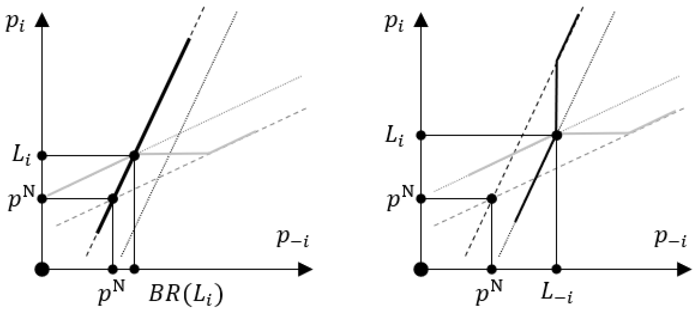
In an asymmetric SPNE, price announcement L i of i must satisfy two conditions. First, it must be non-binding, i.e., L i   p F . Second, it must be such that firm i does not want to deviate and announce L i = B R L i , i.e., π B R L i , L i π L . Clearly, L i = 0 satisfies these two conditions so that these asymmetric SPNE always exist. Figure A1 (left) provides a stylized example of firm’ best response functions for the on-path pricing subgame in an asymmetric SPNE. Firm i is unrestricted, and its second-stage best-response function R p i , L i coincides with B R p i ; it is the solid black curve. Firm i is restricted by L i , and its second-stage best-response function R p i , L i is shown by the solid grey curve.
Equilibria where neither of the firms is unrestricted.
Let announcements L i , L i followed by prices p i , p i be an SPNE outcome, in which B R p i < L i and B R p i < L i . Both announcements are binding, and each firm is either restricted (when p i z L so that B R ~ p i , γ p i = L i ) or breaking its announcement (when p i < z L so that B R ~ p i , γ = p i < L i ). We show that in an SPNE, p i = z L so that B R ~ p i , γ = p i = L i must hold for both firms.
Suppose p i < z L . Then, the best response of firm i   p i = R p i , L i = B R ~ p i , γ is independent of L i , and firm i has a profitable deviation to reduce its announcement to L i = p i and save deviational cost C = γ L i p i . Hence, it must be that p i = L i and, similarly, p i = L i .
Figure A1. Firms’ best responses and Nash equilibria in on-path subgames for asymmetric (left picture) and symmetric (right picture) SPNE. Best responses B R p are dashed curves that intersect at p i = p i = p N , generalized best responses B R ~ p , γ are dotted curves, the second stage best-response functions R p , L are solid curves; grey (black) curves are of firm i ( i ).
Games 16 00013 g0a1
Suppose B R ~ p i , γ > p i = L i and B R ~ p i , γ p i = L i . Then, the best response of firm i   p i = R p i , L i = L i is independent of p i , and firm i has a profitable deviation to marginally reduce L i to L i = L i ε . Both firms remain restricted. In NE, firm i keeps charging price p i = p i = L i , and firm i lowers its price to p i = L i . This deviation is profitable because profit of firm i , π p i , p i , is decreasing in p i when p i > B R p i . Hence, it must be that B R ~ p i , γ = p i = L i and, similarly, B R ~ p i , γ = p i = L i . Thus, the necessary SPNE condition is L i = B R ~ L i , γ that must hold for both firms. Since B R ~ p , γ is increasing in p and has slope less than one, the equilibrium, if it exists, is unique, symmetric, and determined by L i = L i = L where L = B R ~ L , γ . Figure A1 (right) provides a stylized example of firm’ best response functions for the on-path pricing subgame in a symmetric SPNE. Both firms are restricted, their second-stage best-response functions are solid black (for i ) and grey (for i ) curves.
To determine equilibrium existence conditions, let us consider firm i . Its equilibrium profit is π L , L . Deviating to L i > L forces firm i to break L i so that its best response is p i = B R ~ p i , γ . Since the best response of firm i does not change, NE remains the same, p i = p i = L . This deviation only increases the cost of firm i and is, therefore, not profitable. Deviating to L i < L can either keep firm i restricted, if L i B R L , L , or make it unrestricted, if L i B R L . In both cases, firm i breaks its announcement and has best response p i = B R ~ p i , γ . Profit of firm i equals the generalized price-leader profit π ~ L p i = π p i , B R ~ p i , γ . Function π ~ L p is assumed concave and is, therefore, maximized by some p ~ L 0 , p ¯ . The deviation to L i < L is not profitable if an only if π ~ L L i increases at L i = L , i.e., if p ~ L L . Hence, L p ~ L must hold in equilibrium. Therefore, L = B R ~ L , γ and L p ~ L are the two necessary and sufficient SPNE conditions. Condition L p ~ L implies d d L π ~ L L 0 .
To show that these conditions fail if γ is sufficiently large, we write L = B R ~ L , γ as π p i L , L = γ so that L p ~ L can be written as follows:
0 d d L π ~ L L = π p i L , L γ .
This inequality necessarily fails if γ > max p 0 , p ¯ π p i p , p . As a result, for large γ , the solution L (if it exists) to the equation L = B R ~ L , γ is such that L > p ~ L , and each firm has a profitable deviation to L i = p ~ L . Hence there is some γ ¯ S > 0 such that for any γ > γ ¯ S , no SPNE exist, including all symmetric equilibria, in which both firms make binding announcements. This ends the proof.□
Proof of Proposition 3. 
We consider symmetric and asymmetric SPNE separately.
Asymmetric SPNE.
In an asymmetric SPNE, p i = L i > B R p i and p i = B R L i . In the proof of Proposition 2, a threshold γ ¯ A has been defined in such a way that L i = p L is not an SPNE announcement for some γ < γ ¯ A , because p L , B R p L is not NE in the subgame following L i = p L : firm i has a profitable deviation to charge a price p i < L i . Because any announcement L i > p L also suffers from this deviation, only SPNE where L i < p L may exist. Consider such an SPNE.
Let announcements L i , L i followed by prices p i , p i be an SPNE where L i < p L . Announcement L i is restrictive so that B R p i < L i . Firm i must be restricted so that B R ~ p i , γ p i = L i . If B R ~ p i , γ > p i , a marginal deviation to L i = p i + ε is profitable because firm i remains restricted and its profit π L i , B R L i = π L L i is increasing in L i for L i < p L . Hence, it must be that B R ~ p i , γ = p i = L i . Using p i = B R p i , we write it as B R ~ B R L i , γ = L i , Since the left-hand side is continuously increasing in L i , γ and has a slope less than one in L i , the solution L i = p A γ is unique and is continuously increasing in γ . Since p A 0 = p N and p A γ ¯ A = p L , p A γ exists for all γ 0 , γ ¯ A . This proves part 1 of the proposition.
Symmetric SPNE.
In a symmetric SPNE, L i = L i = p S where p S = B R ~ p S , γ . In the proof of Proposition 2, a threshold γ ¯ S is defined in such a way that for any γ > γ ¯ S , equation B R ~ p S , γ = p S has no solution p S that satisfies p S p ~ L , where p ~ L 0 , p ¯ is a maximizer of π ~ L p = π p , B R ~ p , γ . Thus, γ ¯ S is the largest solution to the equation B R ~ p ~ L , γ = p ~ L . Assume γ < γ ¯ S in the rest of the proof.
Since the left-hand side of the equation B R ~ p , γ = p is continuously increasing in p , γ and has a slope less than one in p , its solution p S γ is unique and is continuously increasing in γ . Since p S 0 = p N < p ~ L 0 = p L , equilibrium condition p S γ p ~ L γ holds at γ = 0 . By continuity, it holds for γ 0 , γ _ S where γ _ S 0 , γ ¯ S is the smallest solution to the equation B R ~ p ~ L , γ = p ~ L . By construction, the symmetric SPNE always exists for γ 0 , γ _ S γ ¯ S , never exist for γ > γ ¯ S , and only exist for γ γ _ S , γ ¯ S if p S γ p ~ L γ . This ends the proof of part 2.
Finally, since B R ~ p N , γ = B R ~ B R p N , γ and B R p < p for p > p N , it follows that the B R ~ p , γ > B R ~ B R p , γ for p > p N .Therefore, p S γ , which is the solution to p S γ = B R ~ p S , γ , is always larger than p A , which is the solution to p A = B R ~ B R p A , γ , i.e., p S γ > p A γ for any γ . This ends the proof.□
Proof of Lemma 2. 
Similar to the proof of Lemma 1, for any announcement L i , H i , we define price thresholds z L , y L , y H , and z H , which depend on L i and H i , as follows:
B R y L = L i , B R y H = H i , π B R z L , z L β = π L i , z L , π B R z H , z H β = π H i , z H .
If an equality above never holds, we set the corresponding price threshold to either 0 or to p ¯ . Thresholds y L and y H are unique because of the monotonicity of B R p i . Threshold z L is uniquely determined by G z L , L = β , where:
G z , A π B R z , z π A , z ,
because of the monotonicity of G z , A on z < y L :
G z z , L = π p i B R z , z π p i π L , z < 0 .
The inequality follows from 2 π p i p i > 0 and B R z < L for z < y L . Similarly, threshold z H is uniquely determined by G z H , H = β .
When p i y L , y H so that firm i is unrestricted, R i = B R p i . When it is restricted, then either R i = L i if p i z L , y L or R i = H i if p i y H , z H . Otherwise, firm i breaks its announcement so that R i = B R p i .
Firm i is restricted when either G p i , L < β or G p i , H < β , and it breaks the announcement when G p i , L > β or G p i , H > β . When G p i , L = β or G p i , H = β , the firm is indifferent between these two options and, therefore, has two best responses. This occurs when p i z L , z H .
Best response R i = R p , L i , H i is non-decreasing in p . It has a slope less than 1 for all values of p when it is continuous. Therefore, NE always exists, yet is not necessarily unique. Since R i is piecewise continuous with three intervals of continuity at most, the number of equilibria is finite.□
Proof of Proposition 4. 
As in the proof of Proposition 2, both firms cannot be unrestricted in an SPNE, and cannot break their announcements. First, we consider an SPNE where only one firm is restricted, then we turn to an SPNE where both firms are restricted.
Equilibria where one firm is restricted.
Let announcements L i , L i followed by prices p i , p i be an SPNE outcome, in which firm i is restricted so that p i = L i , and firm i is unrestricted so that p i = B R L i . Firm i gets profit π L i , B R L i , the profit of the Stackelberg leader. Consider a subgame after firm i deviates and announces L i . According to the equilibrium selection requirement 2, if L i p N the firm i gets profit π p N , p N , otherwise firm i is either restricted and gets profit π L i , B R L i if L i , B R L i is NE, or firm i breaks its announcement and gets profit π p N , p N β in NE p N , p N . Maximizing deviational profit π L i , B R L i of firm i w.r.t. deviational announcement L i we obtain that the best deviation is L i = p L . Therefore, L i = p L followed by prices p L , p F is an SPNE outcome if p L , p F is the NE of the subgame, i.e., if π L p L π B R p F , p F β . Hence, if β > β ¯ A where:
β ¯ A π   B R p F , p F π L p L ,
then L i = p L is an SPNE announcement. The two conditions of Proposition 4 that L i must satisfy in an SPNE are the same as in Proposition 2. Figure A2 (left) provides a stylized example of firm’ best response functions for the on-path pricing subgame in an asymmetric SPNE. The second stage best-response function p i = R i p i , L i is discontinuous and multi-valued at p i = B R L i . As a result of this discontinuity, on-path subgame has two NE: L i , B R L i and p N , p N . On path, NE L i , B R L i is played.
Equilibria where both firms are restricted.
Let announcements L i , L i followed by prices p i , p i = L i , L i be an SPNE outcome, in which B R L i < L i and B R L i < L i . Both firms are restricted so that π L i , L i π B R L i , L i β and p i = L i . Similar to the proof of Proposition 2, we show that π L i , L i = π B R L i , L i β .
Suppose, on the contrary, that π L i , L i > π B R L i , L i β , as is shown on Figure A2 (middle). The subgame has two NE: L i , L i and p N , p N ; NE L i , L i is on path. Inequality π L i , L i > π B R L i , L i β is equivalent to z L < L i where p = z L is the point of discontinuity of R i p , L i defined by π L i , z L = π B R z L , z L β . We can now see that firm i has a profitable deviation L i = L ^ z L , L i . Consider a subgame following announcements L i , L ^ .   The second stage best-response function p i = R p i , L ^ of firm i   is shown by a bold dotted black curve. There are two NE in this subgame: L i , L ^ and p N , p N ; these are the intersections of this dotted black curve p i = R p i , L ^ and the solid gray curve p i = R p i , L i .
According to the equilibrium selection requirement 2, NE of this subgame is L i , L ^ . Profit of firm i in this deviation is π L ^ , L i > π L i , L i because (1) π p i , L i decreases with p i on p i > B R L i , and (2) L ^ B R L i , L i as it can be seen on Figure A2 (middle). Thus, π L i , L i = π B R L i , L i β must hold for both firms. Figure A2 (right) presents this case. The on-path subgame has two NE: L i , L i and p N , p N . On path, NE L i , L i is played.
Using function G z , A , which is defined in the proof of Lemma 2:
G z , A π B R z , z π A , z ,
we write the necessary SPNE conditions π L i , L i = π B R L i , L i β as G L i , L i = β and G L i , L i = β .
In order to see that the equilibrium is necessarily symmetric, we note that for the relevant range of the arguments, i.e., for A = L and z < y L so that B R z < L , G z , A is decreasing in z (this is shown in the proof of Lemma 2) and is increasing in A . Hence, the equilibrium equation G L i , L i = β defines L i as a continuously increasing function of L i , i.e., L i = F L i , β . Similarly, L i = F L i , β . In equilibrium, both conditions L i = F L i , β and L i = F L i , β must hold. Suppose that there is an asymmetric SPNE L i , L i = L 1 , L 2 with L 1 > L 2 . Then, both conditions L 1 = F L 2 , β and L 2 = F L 1 , β must hold for L 1 > L 2 , which contradicts the monotonicity of F . Thus, the equilibrium, if it exists, is necessarily symmetric, L i = L i = L , and is determined by condition G L , L = β :
π B R L , L π L , L = β .
Figure A2. Firms’ best responses and Nash equilibria in on-path subgames for asymmetric (left picture) and symmetric (right picture) SPNE. The middle picture illustrates why π L i , L i > π B R L i , L i β cannot happen on path in a symmetric SPNE. Best responses B R p are dashed curves that intersect at p i = p i = p N , the second stage best-response functions R p , L are thick solid curves, z L is the point of discontinuity of R p i , L i , grey (black) curves are of firm i ( i ).
Games 16 00013 g0a2
This condition necessarily fails for β > max p 0 , p ¯ π B R p , p π p , p . Hence, there is some β ¯ S > 0 such that for any β > β ¯ S , no SPNE exist, including all symmetric equilibria, in which both firms make binding announcements. This ends the proof.□
Proof of Proposition 5. 
We consider symmetric and asymmetric SPNE separately.
Asymmetric SPNE.
In an asymmetric SPNE, p i = L i > B R p i and p i = B R L i . In the proof of Proposition 4, a threshold β ¯ A has been defined in such a way that L i = p L is not an SPNE announcement for some β < β ¯ A . Consider an SPNE where L i < p L .
Let announcements L i , 0 followed by prices p i , p i be an SPNE where L i < p L and p i = B R p i . Firm i is restricted by L i so that B R p i < L i = p i and:
π   L i , B R L i π B R B R L i , B R L i β .
Profit of firm i in this SPNE is π L L i = π   L i , B R L i , which is increasing in L i for L i < p L . This implies that if L i < p A then firm i has a profitable deviation L i = p A (similar to the proof of Proposition 4, we use the equilibrium selection requirement 2 for making this argument). Hence, L i = p A must hold.
To show that p A β   is well defined and increasing, we consider a function x p , β , x p , β B R p , implicitly defined by:
π x , p = π B R p , p β .
Function x p , β is well defined on β < β ¯ A and is increasing:
x β = π p i x , p 1 > 0 ,
because x p , β > B R p > p N for β > 0 and p > p N so that π p i x , p < 0 , and:
x p = π p i B R p , p π p i x , p π p i x , p = B R p x 2 π t , p p i p i d t B R p x 2 π t , p p i 2 d t ε , 1 ε ,
because of the assumption 2 π p i p i / 2 π p i 2 ε , 1 ε .
An SPNE announcement p A β is a solution to p A = x B R p A , β , i.e., a fixed point of x B R p , β , and p A β ¯ A = p L by construction. Since x p N , β > p N , for any β 0 , β ¯ A there is a unique solution p A β p N , p L that is increasing in β . This proves part 1 of the proposition.
Symmetric SPNE.
In a symmetric SPNE, L i = L i = p S , where p S satisfies:
π p S , p S = π B R p S , p S β .
In the proof of Proposition 4, a threshold β ¯ S has been defined in such a way that for any β > β ¯ S , this equation does not define an SPNE announcement p S . Assume β 0 , β ¯ S in the rest of the proof.
The symmetric SPNE announcement p S β is the unique solution of p S = x p S , β and satisfies p S > p N . The asymmetric SPNE announcement p A β is the unique solution of p A = x B R p A , β , and it also satisfies p A > p N . Since B R p < p for p > p N , it follows that x B R p , β < x p , β . As a result, p A β , the fixed point of x B R p , β , is always smaller than p S β , the fixed point of x p , β : p A β < p S β . This proves part 3 of the proposition.
In a symmetric SPNE, firms’ profit is π p S , p S . It can be seen in Figure A2 (right), that any deviation to L i > p S and a marginal deviation to L i < p S result in a subgame with the unique ‘normal’ NE p N , p N . Indeed, when L i increases, the point of discontinuity of the second-stage best-response function p i = R p i , L i (solid grey curve) shifts to the left. When L i marginally decreases, this point of discontinuity shifts to the right, but the horizontal part of the graph shifts downwards. In both cases, p N , p N is the unique NE after these deviations. Since p S > p N :
π p S , p S = π B R p S , p S β > π B R p N , p N β = π p N , p N β .
Therefore, neither of these deviations are profitable. Only infra-marginal deviations to L i < p S that lead to subgames with NE L i , B R L i can be profitable. Deviational profit of firm i is π L i , B R L i = π ~ L L i , 0 which increases on L i p N , p L . Hence, the most profitable deviation is either L i = p L if β β ¯ A or L i = p A if β < β ¯ A .
This implies that if β β ¯ A , then p S is an SPNE announcement if and only if:
π p S , p S π p L , B R p L = π p L , p F ,
and if β β ¯ A , then p S is an SPNE announcement if and only if:
π p S , p S π p A , B R p A .
To show that a symmetric SPNE exists for small values of β , we write:
p S , p S = π B R p S , p S β ,   π p A , B R p A = π B R B R p A , B R p A β ,
so that
π p S , p S π p A , B R p A = π B R p S , p S π B R B R p A , B R p A     = π F p S π F B R p A > 0 ,
where π F p = π B R p , p , because π F p is increasing and p S > p A > B R p A . Hence, the deviation to L i = p A is not profitable for all β β ¯ A .
This implies that there exists a β _ S β ¯ A , β ¯ S such that for all β < β _ S , p S exists and is an SPNE announcement. This proves part 2 of the proposition.
To prove part 4, we consider functions p A β and p S β , and the defining them equations G A p = 0 and G S p = 0 . At β = 0 , they result is p A 0 = p S 0 = p N , and in derivatives:
d G A d p p N = d G S d p p N = π p i π   p N , p N = 0 ,
due to π p i B R p , p = 0 (this is the first-order condition that defines B R p ) and π p i p N , p N = 0 (this is the definition of p N ). Since p A β and p S β are the inverses of G A p and G S p correspondingly, their derivatives at β = 0 are infinite. Derivatives of the asymmetric equilibrium profits at β = 0 are also infinite:
d π i d β = d d β π p A , B R p A = π p i p N , p N B R p N d p A d β , d π i d β = d d β π B R p A , p A = π p i p N , p N d p A d β .
Derivatives of the symmetric equilibrium profits at β = 0 are infinite as well:
d π i d β = d π i d β = d d β π p S , p S = π p i p N , p N d p S d β .
This ends the proof.□
Cost Thresholds.
For the numerical example used in this paper, cost thresholds are given by:
γ ¯ A = 2 b + 3 d d 2 4 2 b + d 2 d 2 b + d , γ _ S = γ ¯ S = d 2 2 b 2 b + 3 d + d 2 > γ ¯ A , β ¯ A = d 4 2 b + 3 d 2 64 b + d 3 2 b + d 2 d 2 2 , β _ S = β ¯ S = d 4 b + d b b + d + b + d b d 2 2 2 b + d 2 d 2 2 > β ¯ A .

Notes

1
See the European Commission Decision of 21 February 2007 in Case COMP/E-1/38.823—PO/Elevators and Escalators.
2
See the European Commission Provisional Decision of 27 September 2017 in Case AT.39824—Trucks.
3
See the 2004 Decision of the Director-general of the Dutch competition authority in Case Number 1615/691 (Fietsfabrikanten), in Dutch.
4
See Ross (1992) for the role of product differentiation.
5
This phenomenon sometimes occurs in the literature, e.g., in van Damme and Hurkens (1999) and Reynolds and Wilson (2000).
6
When π p i y , p > γ (or π p i y , p < γ ) for any y , we define B R ~ p , γ = p ¯ (or B R ~ p , γ = 0 ).
7
This holds when B R c > c and 2 π p i 2 1 2 π p i p i ε , 1 ε for some ε > 0 , and we assume that.
8
This holds when π ~ L p , γ is concave in p , and we assume that.

References

  1. Cabral, L. (2000). An introduction to industrial organization. MIT Press. [Google Scholar]
  2. Church, J., & Ware, R. (2000). Industrial organization: A strategic approach. McGraw-Hill. [Google Scholar]
  3. García Díaz, A., González, R. H., & Kujal, P. (2009). List pricing and discounting in a bertrand–edgeworth duopoly. International Journal of Industrial Organization, 27(6), 719–727. [Google Scholar] [CrossRef]
  4. Gill, D., & Thanassoulis, T. (2016). Competition in posted prices with stochastic discounts. The Economic Journal, 126(594), 1528–1570. [Google Scholar] [CrossRef]
  5. Harrington, J. E., Jr. (2022). The anticompetitiveness of a private information exchange of prices. International Journal of Industrial Organization, 85, 102793. [Google Scholar] [CrossRef]
  6. Harrington, J. E., Jr., & Ye, L. (2019). Collusion through coordination of announcements. The Journal of Industrial Economics, 67(2), 209–241. [Google Scholar] [CrossRef]
  7. Lubensky, D. (2017). A model of recommended retail prices. RAND Journal of Economics, 48(2), 358–386. [Google Scholar] [CrossRef]
  8. Raskovich, A. (2007). Competition or collusion? Negotiating discounts off posted prices. International Journal of Industrial Organization, 25(2), 341–354. [Google Scholar] [CrossRef]
  9. Reynolds, S., & Wilson, B. J. (2000). Bertrand–edgeworth competition, demand uncertainty, and asymmetric outcomes. Journal of Economic Theory, 92(1), 122–141. [Google Scholar] [CrossRef]
  10. Ross, T. W. (1992). Cartel stability and product differentiation. International Journal of Industrial Organization, 10, 1–13. [Google Scholar] [CrossRef]
  11. van Damme, E., & Hurkens, S. (1999). Endogenous price leadership. Games and Economic Behavior, 47(2), 404–420. [Google Scholar] [CrossRef]
Figure 1. Absolute price differences p L p N , and p F p N , represented by the dashed and solid curves, respectively, as functions of the parameter d for linear demand with b = 1 and c = 0 .
Games 16 00013 g001
Figure 2. Relative price differences p L p N p N and p F p N p N , represented by the dashed and solid curves, respectively, as functions of the parameter d for linear demand with b = 1 and c = 0 .
Games 16 00013 g002
Figure 3. Relative profit differences π L π N π N , and π F π N π N , represented by the dashed and solid curves, respectively, as functions of the parameter d for linear demand with b = 1 and c = 0 .
Games 16 00013 g003
Figure 4. Absolute price differences p A p N for the leader, B R p A p N for the follower, and p S p N , represented by the dashed, solid, and dotted curves, respectively, as functions of the cost parameter γ , for linear demand with c = 0 and b = d = 1 .
Games 16 00013 g004
Figure 5. Absolute profit differences π i A π N , π i A π N , and π S π N , represented by the dashed, solid, and dotted curves, respectively, as functions of the cost parameter γ , for linear demand with c = 0 and b = d = 1 .
Games 16 00013 g005
Figure 6. Absolute price differences p A p N , B R p A p N , and p S p N , represented by the dashed, solid, and dotted curves, respectively, as functions of the cost parameter β , for linear demand with c = 0 and b = d = 1 .
Games 16 00013 g006
Figure 7. Absolute profit differences π i A π N , π i A π N , and π S π N , represented by the dashed, solid, and dotted curves, respectively, as functions of the cost parameter β , for linear demand with c = 0 and b = d = 1 .
Games 16 00013 g007
Disclaimer/Publisher’s Note: The statements, opinions and data contained in all publications are solely those of the individual author(s) and contributor(s) and not of MDPI and/or the editor(s). MDPI and/or the editor(s) disclaim responsibility for any injury to people or property resulting from any ideas, methods, instructions or products referred to in the content.