Asymmetric Information and Credit Rationing in a Model of Search

Abstract

This paper presents a competitive search model focusing on the impact of asymmetric information on credit markets. We show that limited entry by lenders results in endogenous credit rationing, which, in turn, plays a key role in managing adverse selection and prevents the credit market from collapsing.

1. Introduction

In credit markets, informational asymmetry arises when financiers cannot assess the success potential of entrepreneurs, leading to adverse selection. When entrepreneurs differ in terms of their probability of success (Stiglitz & Weiss, 1981), this information gap creates a scenario similar to what Akerlof (1970) termed the “lemons problem”, which can ultimately cause the credit market to collapse.

With this issue in mind, this paper focuses on how market participants interact with each other and how this may impact the issue of adverse selection. Traditional models frequently assume a Walrasian market, where matches between creditors and entrepreneurs are instantaneous and frictionless. By contrast, our paper adopts a directed/competitive search model in the tradition of Guerrieri et al. (2010), capturing the decentralized and frictional characteristics, which are typical in real-world credit markets.

We consider an economy with homogeneous, risk-neutral lenders and heterogeneous entrepreneurs seeking financing for investment projects. Entrepreneurs differ in their likelihood of success: high types have a greater chance of success, while low types are less likely to succeed. Lenders simultaneously and independently post contracts specifying collateral and interest rate terms. After observing all available contracts, borrowers direct their search to the most favorable option. Each lender can finance only one project. Given the decentralized nature of the matching process and the capacity of each lender, some lenders may receive no applications, and some borrowers may not secure financing.

Under complete information, where lenders can accurately distinguish between entrepreneur types, contracts are tailored to each type’s risk profile. High-type entrepreneurs receive favorable contracts with relatively low collateral and interest requirements. Low types, on the other hand, face contracts that account for their greater risk. Crucially, the separating equilibrium comes with full credit allocation without rationing. This is because, in equilibrium, sufficiently many lenders enter the market for each type. The favorable terms incentivize low types to misrepresent themselves; however, with complete information, this is not an issue as lenders can tell who is who.

Under incomplete information, lenders cannot identify the different types, so they design separating contracts with interest rates and collateral requirements that encourage self-selection. The key problem is to disincentivize low types from misrepresenting themselves. This issue is resolved in two ways: First, high-type contracts are fully collateralized, i.e., lenders demand the maximum possible collateral as part of such contracts. While this demand does not deter high types, it discourages low types due to their greater risk of failure. Second, and more importantly, only a limited number of lenders enter the high-type market and offer credit, restricting the availability of such contracts. This limitation in supply results in credit rationing and discourages low types from making an application.1 Ultimately, credit rationing, coupled with fully collateralized loan requirements, prevents the credit market from collapsing because otherwise, it is impossible to distinguish between the different types and prevent adverse selection.

Endogenous credit rationing is not always enough to keep the market operational, though: an intermediate scenario arises where low types have success probabilities too small to justify tailored contracts for them, but still large enough that they pursue high-type contracts.2 In this region, lenders cannot prevent them from applying for high-type contracts. Consequently, the market collapses, as lenders cannot offer any contract without being exposed to adverse selection.

Related Literature. Our paper is broadly related to the vast literature on asymmetric information in credit markets, which has evolved significantly since Akerlof (1970)’s seminal work on the “lemons problem”, e.g., see Stiglitz & Weiss (1981), Bester (1985), or Besanko & Thakor (1987), among many others. We differ from these studies by considering a fundamentally different market setup that incorporates search and matching, as opposed to a frictionless Walrasian market.

Our model is based on a competitive search framework in the tradition of Burdett et al. (2001), Wright et al. (2021), or more recently Selcuk (2024). The paper by Guerrieri et al. (2010) incorporates asymmetric information into a competitive search setup and explores how adverse selection in such an environment can be managed. Our paper extends this line of research by specifically analyzing credit markets, where the interaction between search frictions and asymmetric information creates equilibrium outcomes with credit rationing.

Additionally, our work is related to the literature on search models in credit markets, such as Vesala (2007), who examine market liquidity and competition under asymmetric information; Dong et al. (2016), who analyze credit rationing under search frictions (but with no asymmetric information); and Davoodalhosseini (2019), who further examines the efficiency of the equilibrium in Guerrieri et al. (2010). We contribute to this line of work by focusing on endogenous credit rationing and collateral requirements, and how they can be used to manage informational asymmetry in a decentralized market setting.

2. Model Setup

The economy consists of a continuum of heterogeneous borrowers (entrepreneurs) and homogeneous lenders. Each lender has $1 available to lend and must choose between entering the credit market or staying out. Entering the market involves lending to an entrepreneur who undertakes a risky project. Alternatively, by staying out, a lender can invest in a risk-free asset with a guaranteed return of $1+t$.

Each entrepreneur requires $1 to finance their project. If successful, a project yields a payoff of $1+g$. The probability of success depends on the entrepreneur’s type: high-type entrepreneurs have a success probability of $p_h$, while low-type entrepreneurs have a success probability of $p_l$, with $p_h>p_l$.

Entrepreneurs possess illiquid assets, which cannot be used directly for financing but can be pledged as collateral to secure a loan from lenders. Lenders offer contracts defined by an interest rate $r\in (0,g)$ and a collateral requirement c. The collateral requirement can range from 0 to $1, corresponding to no collateral or full collateralization, or any value in between.

The search process for matching lenders with borrowers occurs in the form of directed search (Guerrieri et al., 2010): First, lenders simultaneously announce contract terms $(r,c)$. After observing the available contracts, borrowers select one to apply. Once matching takes place and the contracts are awarded, projects commence, and eventually, payoffs are realized. Successful projects return $1+g$, while failed projects lead to forfeiture of the pledged collateral.

Our focus will generally be on separating equilibria, where some creditors target high types while others cater to low types. Let ${\theta }_i$ represent the lender-to-entrepreneur ratio (also called “market tightness”) in the market for type $i=h,l$ entrepreneurs.3 These parameters are determined endogenously through free entry by lenders. For instance, if no lender is willing to lend to low-type borrowers, then ${\theta }_l=0$, which effectively shuts down the market for low types. This decision would naturally impact the market for high types as well (more on this later). The probability that a borrower finds a lender in market i is given by

$$\mu \left({\theta }_i\right)=min\{{\theta }_i,1\}.$$

Similarly, the probability that a lender finds an entrepreneur is $\mu \left({\theta }_i\right)/{\theta }_i$. If ${\theta }_i>1$, all entrepreneurs are matched with lenders, though some lenders will remain unmatched. Conversely, if ${\theta }_i<1$, all lenders are assured a match with an entrepreneur, while some entrepreneurs will not secure financing.4 This shortage of credit for entrepreneurs when ${\theta }_i<1$ reflects credit rationing. Thanks to the functional form of $\mu \left({\theta }_i\right)$, every participant on the “short side” of the market is guaranteed a match. Importantly, the short side is not exogenous, but instead, it is determined endogenously via ${\theta }_h$ and ${\theta }_l$.

3. Complete Information

With complete information, lenders can distinguish between borrower types. The utility function of a type i borrower is given by

$$U_i(r_i,c_i,{\theta }_i)=\mu \left({\theta }_i\right)\left[p_i\left(1+g-r_i\right)+\left(1-p_i\right)\left(1-c_i\right)\right]+1-\mu \left({\theta }_i\right).$$

(1)

With probability $\mu \left({\theta }_i\right)$, the borrower can access credit. If the project is successful (with probability $p_i$), the borrower retains a payoff of $1+g$ after repaying the interest $r_i$. Conversely, if the project fails (with probability $1-p_i$), the borrower forfeits their collateral $c_i$ and retains $1-c_i$. The term $1-\mu$ accounts for the scenario where the borrower cannot find a lender, in which case they keep their entire collateral value of 1.

The profit for a lender targeting type i borrowers is equal to

$${\pi }_i(r_i,c_i,{\theta }_i)={\displaystyle \frac{\mu \left({\theta }_i\right)}{{\theta }_i}}\left[p_i\left(1+r_i\right)+\left(1-p_i\right)c_i\right]+1-{\displaystyle \frac{\mu \left({\theta }_i\right)}{{\theta }_i}}.$$

(2)

The term $\mu /{\theta }_i$ represents the probability that a lender meets a borrower. If a borrower is found and the project succeeds (with probability $p_i$), the lender receives back their initial loan amount 1 plus interest $r_i$. If the project fails (with probability $1-p_i$), the lender retrieves the collateral $c_i$. Finally, the term $1-\mu /{\theta }_i$ captures the situation where the lender cannot find a borrower, in which case they retain their capital amount of 1.5

We focus on a separating equilibrium in which some creditors target high types, while others cater to low types. A representative lender operating in market i solves

$$\begin{array}{cc}\hfill & {\overline{U}}_i=\underset{{\theta }_i,r_i,c_i}{max}{U}_i(r_i,c_i,{\theta }_i)\mathrm{subject}\mathrm{to}:\hfill \\ \hfill & \left(\mathrm{i}\right){\pi }_i(r_i,c_i,{\theta }_i)=1+t,\hfill \\ \hfill & \left(\mathrm{ii}\right)U_i(r_i,c_i,{\theta }_i)\ge 1.\hfill \end{array}$$

(P–CI)

Note that there are two problems in (P–CI), one for high types and one for low types. The solution to these problems defines the separating equilibrium, which is characterized by the market tightness for each borrower type, ${\theta }_i$, and contract terms $r_i$ and $c_i$, such that creditors compete to offer each type the highest possible payoff, denoted by ${\overline{U}}_i$. This competition is subject to two key constraints: (i) a free entry condition, which ensures that each lender earns a profit equal to the return from the risk-free asset6, and (ii) a participation constraint, which guarantees that borrowers will only take out a loan if their expected utility from receiving credit is at least as large as their utility from holding onto their illiquid collateral. Note that we do not need an incentive compatibility constraint here because, with complete information, creditors can identify borrower types.

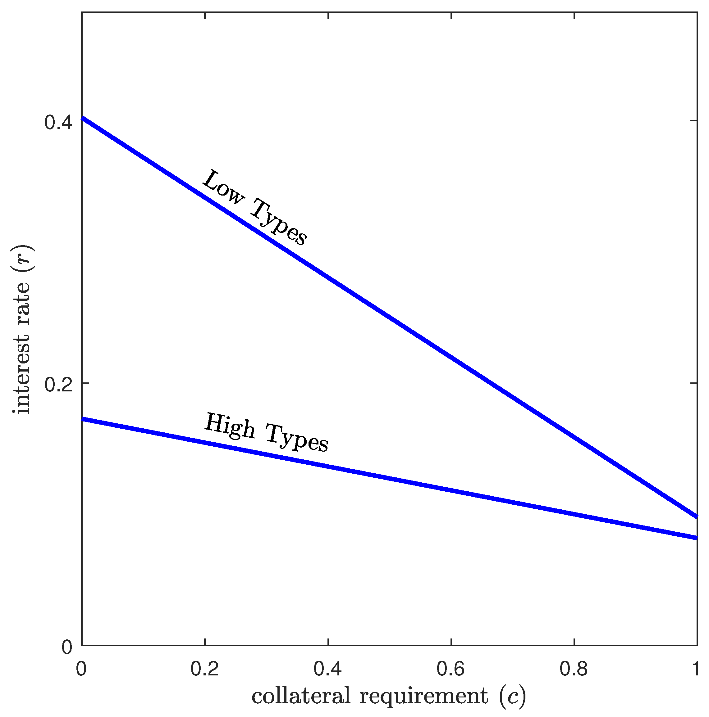
Proposition 1. 

Credit is available to types $i=h,l$ as long as their probability of success is sufficiently high, i.e., $p_i\ge {\displaystyle \frac{1+t}{1+g}}$. Assuming this condition, the optimal level of entry in each market is ${\theta }_i^{*}=1$, ensuring that credit rationing does not occur for either type. The optimal contracts $(r_i^{*},c_i^{*})$ satisfy

$$r_i^{*}={\displaystyle \frac{t}{p_i}}+{\displaystyle \frac{1-p_i}{p_i}}\left(1-c_i^{*}\right).$$

(3)

Sellers targeting high types offer credit with lower interest rates and/or reduced collateral requirements, while those targeting lower types offer credit with higher interest rates and/or stricter collateral conditions, as shown in Figure 1. Lower types have the incentive to misrepresent themselves to take out the more favorable contracts, however, with complete information, this is not an issue for lenders.

An important feature of the complete information setting is the fact that ${\theta }_h^{*}={\theta }_l^{*}=1$, which allows access to credit for both types without rationing. Thanks to their ability to distinguish between different entrepreneur types, lenders have no incentive to limit credit access; however, as we will see, this changes in a setting with incomplete information.

The participation condition $p_i\ge (1+t)/(1+g)$ determines whether a borrower will enter the market, where g represents the growth potential of a successful project and t reflects the return from the risk-free asset. If the growth rate g significantly exceeds t, even borrowers with a lower probability of success are inclined to participate due to the high potential payoff. Conversely, if t approaches g, only those with a high probability of success will find it worthwhile to participate.

Finally, partial market participation is also possible: if $p_l<{\displaystyle \frac{1+t}{1+g}}<p_h$ then only high types are offered credit contracts, and low types are excluded from the market. This exclusion poses no issue (i.e., low types do not attempt to pursue high-type contracts) as creditors can reliably identify different types.

4. Incomplete Information

We now examine the setting with incomplete information, where each borrower’s type is private information, making it impossible for creditors to verify their likelihood of success. As in the previous section, we focus on a separating equilibrium. A representative lender catering to low types solves

$$\begin{array}{cc}\hfill & {\overline{U}}_l=\underset{{\theta }_l,r_l,c_l}{max}{U}_l(r_l,c_l,{\theta }_l)\mathrm{subject}\mathrm{to}:\hfill \\ \hfill & \left(\mathrm{i}\right){\pi }_l(r_l,c_l,{\theta }_l)=1+t,\hfill \\ \hfill & \left(\mathrm{ii}\right)U_l(r_l,c_l,{\theta }_l)\ge 1,\hfill \\ \hfill & \left(\mathrm{iii}\right)U_h(r_l,c_l,{\theta }_l)\le {\overline{U}}_h.\hfill \end{array}$$

(P-Low)

This setup resembles the complete information problem in (P–CI) but includes an incentive constraint. If a high-type borrower poses as a low type, they receive payoff $U_h(r_l,c_l,{\theta }_l)$; if they choose their own contract, then they obtain ${\overline{U}}_h$. The incentive constraint in (iii) is required to discourage them from opting for the low-type contracts.

Similarly, the problem for a lender catering to high types is given by

$$\begin{array}{cc}\hfill & {\overline{U}}_h=\underset{{\theta }_h,r_h,c_h}{max}{U}_h(r_h,c_h,{\theta }_h)\mathrm{subject}\mathrm{to}:\hfill \\ \hfill & \left(\mathrm{i}\right){\pi }_h(r_h,c_h,{\theta }_h)=1+t,\hfill \\ \hfill & \left(\mathrm{ii}\right)U_h(r_h,c_h,{\theta }_h)\ge 1,\hfill \\ \hfill & \left(\mathrm{iii}\right)U_l(r_h,c_h,{\theta }_h)\le {\overline{U}}_l.\hfill \end{array}$$

(P-High)

Here, the incentive constraint (iii) is key once again: if a low type attempts to pass as a high type they obtain $U_l(r_h,c_h,{\theta }_h)$. By choosing their designated contract, however, they receive ${\overline{U}}_l$. To ensure incentive compatibility we need $U_l(r_h,c_h,{\theta }_h)\le {\overline{U}}_l$.

Now consider the larger problem (P) of solving (P-Low) and (P-High) simultaneously. A separating equilibrium is a tuple $({\theta }_h,{\theta }_l,r_h,r_l,c_h,c_l)$ that solves the general problem (P). In what follows, we characterize this equilibrium in detail. Start with (P-Low). We conjecture, to be verified later in the Appendix A, that high types would not want to join a contract for low types, thus the incentive constraint (iii) is slack. In the absence of (iii), (P-Low) is identical to (P–CI), which we solved in the previous section. The solution, therefore, entails

$${\theta }_l^{*}=1,r_l^{*}={\displaystyle \frac{t}{p_l}}+{\displaystyle \frac{1-p_l}{p_l}}(1-c_l),{\overline{U}}_l=p_l(1+g)-t.$$

(4)

We now turn to the second problem involving high types.

Lemma 1. 

The incentive constraint in (P-High) must hold with equality.

The proof is by contradiction: consider an outcome where the incentive constraint (iii) is slack. Absent (iii), the problem in (P-High) is the same as the problem in (P–CI), therefore the resulting contracts are also identical. Recall that in (P–CI) the contract for high types is more favorable, as such low types have an incentive to misrepresent themselves. In Appendix A, we show that without the incentive constraint, lower types would indeed choose to pass as high types, causing the equilibrium to collapse; a contradiction. Therefore (iii) must hold with equality. We can now proceed to characterize the equilibrium.

Proposition 2. 

Under incomplete information, there exists a separating equilibrium characterized by the following:

• Low types experience no credit rationing, i.e., ${\theta }_l^{*}=1$. Their contracts satisfy (4), but $c_l^{*}$ is capped at ${\overline{c}}_l$.
• High types face credit rationing, with ${\theta }_h^{*}<1$, where

  $${\theta }_h^{*}={\displaystyle \frac{p_l\left(1+g\right)-t-1}{p_l\left(1+g\right)-\frac{p_l}{p_h}t-1}}.$$
  Their credit offer entails $c_h^{*}=1$ and $r_h^{*}=t/p_h$.

The equilibrium is illustrated in Figure 2, showing the credit offers available to each type. Contracts for high types require full collateralization ($c_h^{*}=1$), which is less discouraging for them given their higher probability of success, while lower types are more cautious about such collateral requirements.7 However, full collateralization alone does not fully prevent lower types from applying. The equilibrium also includes credit rationing for high-type contracts (${\theta }_h^{*}<1$). Together, these features satisfy incentive compatibility and ensure the market remains functional for all participants.

Moreover, it is easy to verify that ${\theta }_h^{*}$ decreases as $p_l$ falls. This implies that as the difference between entrepreneur types widens—reflected by a lower $p_l$—credit availability for high types becomes more limited due to intensified credit rationing. Indeed, as the gap between types grows, the terms offered to low types worsen, giving them greater incentive to mimic high types. In response, creditors further limit the availability of high-type contracts. In this context, credit rationing serves as an effective risk management tool for lenders.

The contracts for low types must satisfy condition (4) as well as $c_l^{*}<{\overline{c}}_l$ to prevent high types from pursuing them. While the high-type contract features more attractive terms, its limited availability has the potential to make the more accessible low-type contracts seem appealing. By capping collateral for low types, thereby keeping interest rates high, creditors remove any incentive for high types to opt for the readily available low-type contracts.

As in the complete information scenario, the existence of equilibrium depends on the condition that $p_l\ge (1+t)/(1+g)$. However, a key difference arises here. In the complete information context, if low types do not meet this threshold, the market for them would collapse, but the market for high types would continue to operate since creditors can distinguish between the two. In the current setup, however, the two markets are interconnected. Therefore, if $p_l$ falls below the threshold, it could result not only in the shutdown of the low-type credit market but potentially in the collapse of the entire market. In what follows, we explore this relationship.

4.1. Shutdown

Proposition 3. 

Suppose low types’ probability of success $p_l$ is below $(1+t)/(1+g)$. Then the credit market shuts down either entirely or partially.

• If $p_l$ is even below $1/(1+g-t/p_h)$ then low types avoid the credit market altogether while the market for high types remains operational. High types face no credit rationing, i.e., ${\theta }_h^{*}=1$. Their contracts satisfy (3), but $c_h^{*}$ is bounded below by ${\underline{c}}_h$.
• If $p_l$ is above $1/(1+g-t/p_h)$ then low types cannot be prevented from applying to contracts designed for high types. Consequently, the separating equilibrium ceases to exist, leading to a complete shutdown of the entire credit market.

If $p_l$ is even below the threshold $1/(1+g-t/p_h)$, the market remains partially open, with only high types receiving credit offers. In this case, low types stay out of the market, while high types are offered contracts with collateral requirements bounded below by a minimum level, ${\underline{c}}_h$. This lower bound on collateral serves to discourage low types from making an application. In this region, lower type entrepreneurs recognize that their probability of success is so low that pursuing a contract intended for high types is simply not worthwhile. The considerable collateral requirement, combined with the minimal chance of success, exposes them to significant risk. If they fail, they would forfeit their collateral, ultimately leaving them in a worse position. Thus, when $p_l$ is sufficiently small, the market functions partially, providing credit exclusively to high types. Figure 3 illustrates this scenario.

If, however, $p_l$ lies above $1/(1+g-t/p_h)$ but still below $(1+t)/(1+g)$, then the market experiences a complete shutdown. The shutdown region lies in an intermediate zone where low types’ probability of success is too small to warrant a contract tailored specifically for them (if they identify as low types), yet not so small that they refrain from attempting to acquire contracts designed for others. In this region, the entire market collapses, as lenders cannot offer any contract without being exposed to adverse selection.

4.2. Pooling Contracts

Up to this point, our focus has been on a separating equilibrium, where each borrower type was offered a distinct credit contract. We now turn our attention to the possibility of a “pooling equilibrium”, in which all types receive the same contract. We will first identify the conditions under which such an outcome is feasible. Subsequently, we will demonstrate that separating contracts dominate pooling contracts, meaning that in the parameter space where a separating equilibrium is viable, the pooling equilibrium will cease to exist (subject to a condition on the percentage of high types among the borrowers).

Suppose that in the existing pool of customers, fraction $\alpha$ are high types, while the remaining $1-\alpha$ are low types. Creditors recognize that they cannot observe the types of borrowers. Instead of working with $p_h$ and $p_l$, they consider the “average” borrower to have a probability of success given by

$$\overline{p}=\alpha p_h+(1-\alpha )p_l.$$

Based on this weighted probability, creditors then offer a generic, average contract to all entrepreneurs. As we will demonstrate, there are parameter regions where this outcome can indeed materialize. However, when it does occur, it benefits low types at the expense of high types. In other words, such an outcome effectively cross-subsidizes lower types while disadvantaging higher types. This dynamic is crucial because it will be key to demonstrating that the pooling equilibrium collapses once separating contracts become available.

The profit of a creditor is given by

$$\tilde{\pi }={\displaystyle \frac{\mu \left(\theta \right)}{\theta }}\left[\overline{p}\left(1+r\right)+\left(1-\overline{p}\right)c\right]+1-{\displaystyle \frac{\mu \left(\theta \right)}{\theta }}.$$

(5)

This is similar to Equation (2) in the previous section, but with the key difference that the creditor does not observe individual $p_i$s and thus uses $\overline{p}$ as a proxy for the probability. Also, $\theta$, r, and c are not type-indexed. The payoff for a type i buyer is given by

$${\tilde{U}}_i=p_i\left(1+g-r\right)+\left(1-p_i\right)\left(1-c\right).$$

(6)

Since lenders cater to a pool, the parameters r and c are uniform for all borrowers. However, the probability of success, $p_i$, remains type-specific, as each borrower type knows their own success probability. For a pooling equilibrium to emerge, we need ${\tilde{U}}_i\ge 1$, since each entrepreneur’s outside option is to simply retain their illiquid collateral and walk away with a utility of 1.

Lemma 2. 

A pooling equilibrium exists if $\overline{p}\ge (1+t)/(1+g)$.

Our goal is to compare the separating and pooling equilibria. A separating equilibrium with active markets for both types exists only if $p_l>(1+t)/(1+g)$. Since $\overline{p}$ is greater than $p_l$, the condition for a pooling equilibrium is satisfied wherever a separating equilibrium exists. Note that because $\overline{p}>p_l$, the parameter region supporting a separating equilibrium is actually broader than the one supporting a pooling equilibrium.

Proposition 4. 

Low types are strictly better off in a pooling equilibrium than in a separating equilibrium. In contrast, high types are worse off in the pooling equilibrium if the fraction of high types is less than a threshold $\overline{\alpha }.$

The pooling equilibrium offers contracts based on the pooling probability $\overline{p},$ which is higher than $p_l$ but lower than $p_h.$ Consequently, low types receive more favorable terms than they would in a separating equilibrium and are clearly better off. As for high types, the opposite is true: they receive worse terms in a pooling equilibrium than they would in a separating equilibrium. However, there is a caveat: in the separating equilibrium, high types face limited availability via credit rationing. Although the terms of a separating equilibrium are more favorable, the limited availability makes the relative performance of the pooling equilibrium dependent on the fraction $\alpha$.

Corollary 1 

(of Proposition 4). If $\alpha \ge \overline{\alpha }$, then the pooling equilibrium is feasible. Conversely, if $\alpha <\overline{\alpha }$, the pooling equilibrium will cease to exist as high types opt for separating contracts instead.

The existence of a pooling equilibrium depends on the presence of a sufficiently large percentage of high types. When $\alpha$ is high, the average probability of success $\overline{p}$ is close to $p_h$. This makes the pooling contract favorable for high types and reduces the incentive for them to seek out separate contracts. In this case, the pooling equilibrium is feasible. However, if $\alpha$ falls below the threshold $\overline{\alpha }$, then $\overline{p}$ is close to $p_l$, which makes the terms of the pooling equilibrium much less appealing for high types. Consequently, they gravitate toward separating contracts (despite their limited availability). This self-selection by high types disrupts the pooling equilibrium and leads to its breakdown.

4.3. Broader Implications for Policymakers

Our results establish that in equilibrium, credit availability can be intentionally limited and accompanied by very high collateral requirements. Even though such an outcome may be restrictive, it plays an important role in ensuring that the market remains functional under asymmetric information. Regulations or policies that try to make credit more widely available or lower collateral requirements could, therefore, unintentionally disrupt this equilibrium dynamics and lead to adverse selection and potential market collapse.

The key takeaway for financial market regulators is that non-intervention may often be the optimal approach in such market settings. By recognizing that credit rationing and demanding collateral requirements are equilibrium features rather than market failures, regulators can avoid unnecessary and harmful interventions. These insights highlight the importance of understanding market mechanisms before attempting to address inefficiencies in credit markets.

5. Conclusions

In this paper, we investigate a credit market with asymmetric information, where lender–borrower interactions are characterized by a decentralized search and matching process. Under complete information, markets for both types are operational and no credit rationing takes place in that there is enough entry into each market.

With incomplete information, however, lenders limit their participation in the high-type market, thus rationing credit for these borrowers. Credit rationing and the requirement for full collateral on high-type contracts deter low types from misrepresenting themselves. This helps sustain a separating equilibrium, ensuring that, even with information asymmetry and lenders’ inability to differentiate types, both markets remain active. This setup not only addresses the challenges of asymmetric information but also shows how credit rationing acts as a key risk management tool in practice.