A Representation for Many Player Generalized Divide the Dollar Games

Abstract

Divide the dollar is a simplified version of a two player bargaining problem game devised by John Nash. The generalized divide the dollar game has $n>2$ players. Evolutionary algorithms can be used to evolve individual players for this generalized game but representation—i.e., a genome plus a move or search operator(s)—must be carefully chosen since it affects the search process. This paper proposes an entirely new representation called a demand matrix. Each individual in the evolving population now represents a collection of n players rather than just an individual player. Players use previous outcomes to decide their choices (bids) in the current round. The representation scales linearly with the number of players and the move operator is a variant of an evolution strategy. The results indicate that this proposed representation for the generalized divide the dollar game permits the efficient evolution of large player populations with high payoffs and fair demand sets.

1. Introduction

Bargaining occurs whenever two or more people must negotiate benefits associated with some economic activity. Nash [1] constructed a nonzero-sum, two player game to study bargaining situations. Divide the Dollar (DD) is a simpler version of Nash’s bargaining game [2,3]. The DD game is of interest because it simply models the structure inherent in many bargaining problems. In a canonical DD game $n=2$ players propose how to split $1. Each player simultaneously submits a demand indicating what fraction of the dollar they want1. If the demands sum to one dollar or less, then each player gets a payoff equal to their demand. However, both players get no payoff if the demand total is more than $1.

There are many ways to split $1. For example, (0.75, 0.20) or (0.48, 0.47) both have the same demand total, but the second split is considered “fairer” because both players get roughly the same payoff. A Nash equilibrium (NE) in a game exists when no player can get a higher payoff by unilaterally changing his strategy. It is easy to show every (integer) split of exactly $1 is a NE. It is difficult to predict human behavior in a subspace filled with NE because there is no a priori reason to favor one NE over another. For example, humans would see a 50:50 split as fairer than say an 80:20 split but preferences are not encoded in a NE.

Ashlock and Greenwood [4] described a Generalized Divide the Dollar (GDD) game which also splits the surplus but it has $n>2$ players. Games with $n>5$ players are called many player games.

It is not easy to train agents whose demands are fair with a demand total near $1. Evolutionary algorithms have a long history of successfully finding good solutions to difficult problems by mimicking neo-Darwinism mechanics. Representation plays a crucial part in determining how successful the search will be. A representation includes both the genome, which encodes problem solutions, and the move or search operator which determines which genotypes can be visited from a given initial population. Ashlock et. al has extensively studied representations in a variety of problem domains [5,6,7,8].

Greenwood and Ashlock [9] described a representation for a 3-player GDD game. The genome was a neural network and two move operators were investigated: differential evolution and a CMA-ES algorithm. Both evolutionary algorithms successfully found good synaptic weight values for the neural networks with a slight advantage in going to the CMA-ES algorithm. The problem is the neural network architecture is practically limited to no more than 4 or 5 player GDD games.

The main contribution of this paper is it describes a proposed representation for many player GDD games that simplifies the search for near-optimal solutions. There is no limitation on n other than it be finite. The genome is a demand matrix where each row gives the demands for all n players. The number of rows depends on how much historical information from previous rounds is recorded. Each row has a fitness value that depends on the standard deviation of the demands (a measure of fairness) and the demand total. An aggregate of the row fitnesses gives the fitness of the demand matrix. This genome scales linearly with the number of players n and a variation of a $(\mu +\lambda )$ evolution strategy [10] is the move operator that finds parameter values. A representation for a 10-player and a 20-player GDD game is described.

The demand matrix as a representation genome is novel for two reasons. There are two approaches to evolutionary game theory: (1) the concept of an evolutionary stable strategy, and (2) explicit modeling of players and observing how strategy frequencies change over time. Spatial games and well-mixed games with replicator dynamics are typical examples of the second approach2. Conversely, the demand matrix is an entirely new representation where each member of the population is a set of n-players rather than a population of individual players. Secondly, it introduces a different perspective on fitness. In most games fitness is tied to player payoffs. That is, fitness is an individual player attribute. With demand matrix representations fitness is still a single value, but it applies to the choices made by a collection of players rather than to individual players. Fitness is now an n-player attribute. It still drives evolution, but it disconnects survival from individual payoffs. The authors are unaware of any previous work using this concept of fitness. The work described here is also completely different from the method used in [9] where individual players were co-evolved.

2. The Importance of Representation

Let $\mathbf{S}$ denote a search space and $\mathbf{G}$ the genome space. An evolutionary algorithm explores the search space $\mathbf{S}$, looking for the best solutions. $\mathbf{G}$ contains all possible solutions to a problem whereas $\mathbf{S}$ may not—i.e., $\mathbf{S}\subset \mathbf{G}$ is typical. A simple example will help fix the idea. Suppose solutions to a problem are encoded as binary strings and let $i=00\dots 0$ and $j=00\dots 1$ be two solutions. Clearly $i,j\in \mathbf{G}$ but whether $i,j\in \mathbf{S}$ depends on the move operator. A move operator determines which solutions can be visited by the search algorithm (in this case, an evolutionary algorithm). If the move operator flips a random bit then $i,j\in \mathbf{S}$ because a search can move from i to j in a finite number of steps. However, if the move operator flips an even number of bits then both i and j cannot be in $\mathbf{S}$ regardless of how many move operations take place. Clearly a representation must contain both a genome definition and a move operator description.

Associated with each $i\in \mathbf{S}$ is a fitness value $f_i$. Fitness is a measure of solution quality; high fit solutions are better solutions. Let $\mathcal{F}=\left\{f_i\mid i\in \mathbf{S}\right\}$. Then $\mathbf{S}\cup \mathcal{F}$ forms a kind of abstract fitness landscape. The search algorithm, using move operators, explores this landscape looking for the peaks as they mark good solutions.

In previous work a representation for GDD players was presented [9]. But that representation is practical only for small games with no more than 4 or 5 players. A new representation allows investigation of many player games. Results for 10 and 20 player GDD games are presented in this paper. The 20 player game is presented to illustrate the method scales linearly.

3. Background

3.1. Bargaining Games

Nash [1] defined a 2-player bargaining situation as any situation where two individuals have an opportunity to collaborate for mutual benefit in more than one way. Bargaining entails making demands or demands until players reach an agreement (or terminates if no agreement is possible) on how to share some surplus generated by the players. Nash goes on to define a bargaining problem game—commonly called the Nash demand game—with 2 players and a set A of alternatives. If the players agree on some alternative $a\in A$, then a is the outcome. If they fail to reach agreement then outcome d is the result. Players have expected utilities, indicating their preferences among the alternatives, and can veto any outcome other than d. Nash derived a unique solution to this problem.

Agastya [11] generalized the Nash bargaining game to n players. He considered a set of $N=\{1,2,\dots ,n\}$ players who form non-empty subsets called coalitions. A real-valued convex characteristic function describes the surplus different coalitions can obtain. At each iteration a randomly chosen member of a coalition bargains with his counterparts from other coalitions. (The chosen member’s demand is for himself, but it must be compatible with the demands of others in the coalition.) Coalitions cannot form unless all of its members demands can be met. Eventually demands may be satisfied for some coalitions but not necessarily all of them.

Newton [12] also studied bargaining games with player coalitions. A player’s strategy consists of a demand and a set of players with whom he is willing to form a coalition. Players can adjust their strategies by changing their demand or by seeking other coalitions guaranteed to produce a higher payoff. A player may identify multiple suitable coalitions. In that case he joins the larger coalition. Fairness was determined by coalition selection.

The DD game, described in the introduction, dates back more than 30 years [2]. It is a special case of the Nash demand game. It elegantly models situations where two players can benefit by making “reasonable” demands but get nothing if they are too greedy. Moreover, it models situations where some surplus is unused. Fairness is determined by the closeness of player’s demands. A key feature is players cannot easily coordinate their demands because the game naturally contains multiple equilibria. Binmore [13] claimed DD is the archetypal version of bargaining problems where the surplus amount is common knowledge. In the canonical DD the surplus is $1.

3.2. Prior DD Research

There are two issues with DD games: (1) every split of exactly $1 is a Nash equilibrium, and (2) any split that totals to $1 + $ϵ$, where $ϵ>0$ is arbitrarily small, completely wastes the resource (both players get nothing). A number of changes have been proposed to address these issues but surprisingly all of those proposed changes fundamentally altered the nature of the DD game.

In the canonical DD game players somewhat temper their demands because they realize high demands increase the odds of getting zero payoff. Several researchers removed that risk. For example Anbarci [14] proposed if two players demand $d_1+d_2>1$, then player i would get a payoff of $f_i{d}_i$ where $f_i=(1-d_i)/d_j$. Each player is guaranteed to get something in return—even when the demand total exceeds $1. demands in the Anbarci game could be in fractions of one cent. This is unrealistic whenever an economic activity involves the physical exchange of money.

Brams and Taylor [2] devised a method to fully distribute the dollar even if the demand totals were less than $1. They also reduced the number of Nash equilibria by making them all payoff equivalent. But now a new problem was introduced: the player with the lowest demand could actually receive almost the entire dollar as a payoff. For instance, demands of (0.98, 0.99) would result in payoffs of (0.98, 0.02).

Rachmilevitch [15] also allowed non-integer demands but this continuous game has only one Nash equilibrium whereas the canonical DD has many Nash equilibria. Additionally rules were derived to split $1 among the players if the demand total exceeded $1.

de Clippel et. al [16] described a DD game for $n>2$ players. However, that game version has little in common with all other DD investigations. In their game players do not submit personal demands but instead issue a report stating what was a fair portion of a dollar that other players deserve. Payoffs are then distributed if a specific division is compatible with an aggregate of all reports. Essentially under this game the payoff to a given player ultimately depends entirely on the opinion of the other players. It is not clear how this approach provides any insight into the bargaining process because players do not submit personal demands.

3.3. The Generalized Divide the Dollar Game

Ashlock and Greenwood [4] defined a GDD game where there are $n>2$ players splitting some dollar amount. GDD preserves all of the features of a canonical DD game: players get their demands if the demand total is less than or equal to $1, and demand totals exceeding $1 result in zero payoff to all players. GDD does allow for a small subsidy—i.e., a small amount above $1 where players can still get their demand. However, this subsidy can only be used if the bids are “fair” in the sense they are roughly equal so no player gets exploited. The objective is to find a set of n fair bids with a bid total as close as possible to $1.

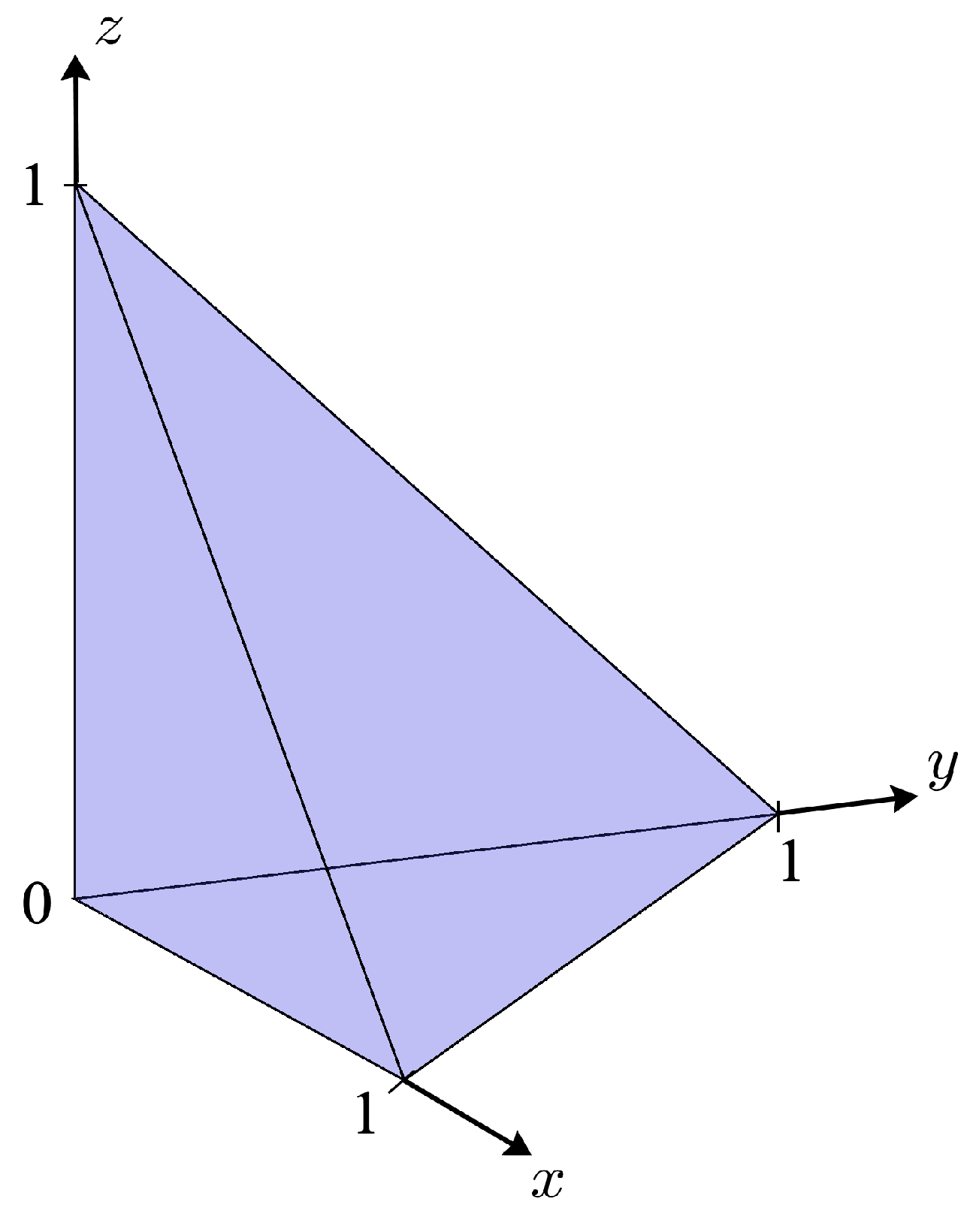
In the generalized game every point in a compact and convex subspace $\mathcal{S}\subset {\mathbb{R}}_{+}^n$ represents a demand total. Each player picks a coordinate of this point and that coordinate specifies the player’s demand. Players are said to be coordinated—i.e., the demand total is ≤ $1—if the point is located on or beneath the surface of an $(n-1)$-simplex. Figure 1 shows the coordinated subspace in ${\mathbb{R}}_{+}^3$.

One minor change was made to the canonical DD game to accommodate many player games. The original GDD work investigated a 3-player game and the amount to be split was $1. But many player games have $n>5$ players. In some many player games fair demands would out of necessity be quite small if the amount split is left at $1. For example, in a $n=20$ player game fair demands would be around 0.05. To get around this problem the amount to be split is increased to $n/2$ dollars. This increase means instead of a simplex vertex at $(0,0,1,0,\dots ,0)$, it is now located at $(0,0,n/2,0,\dots ,0)$. Players are considered coordinated if the sum of their demands is less than or equal to $n/2$ dollars and such demands are said to belong to a coordinated demand set. Choosing a larger dollar amount to split means players can now have a fair demand set without having to make ridiculously low demands. No other game changes were made.

Unlike the Agastya and Newton games, a GDD game is a grand coalition game; each player bargains with the other $n-1$ players. This distinction is important. Coalitions cannot form unless they can satisfy all of its member’s demands. Coalition formation also implies some semblance of fairness (at least within the coalition). It may be possible for some coalitions to satisfy all of its member’s demands, but that does not necessarily guarantee all n players may have their demands met. For instance, a player’s demand may be so high that no coalition it joins can meet all of the member’s demands. Players in both the Agastya and Newton games typically get zero payoff if they are unable to join a coalition. Conversely, in a grand coalition players are forced to adapt their demands until all can be met. Fairness is then measured by computing the standard deviation about the demand mean of all n players.

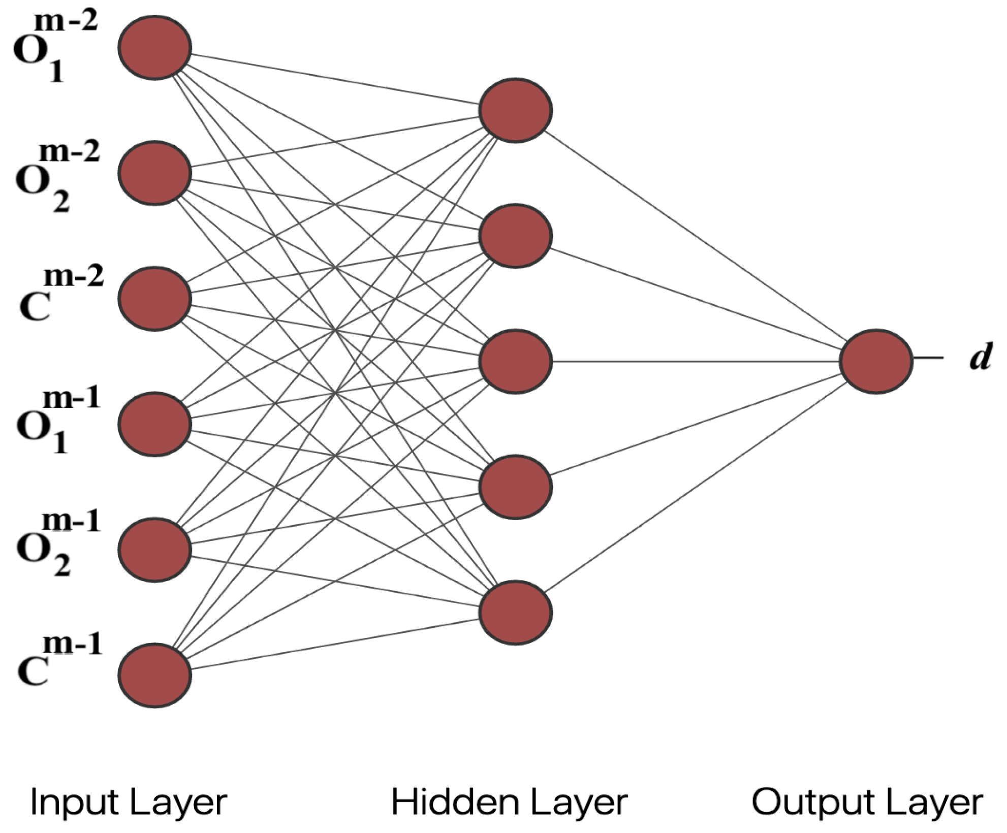
An implementation of a GDD game was described in [9]. The representation consisted of a neural network (NN) for the genome and two evolutionary algorithms for the move operators. The neural network architecture is shown in Figure 2. All synaptic weights were constrained to $[-1.0,1.0]$ with a sigmoid activation function and the output node demand (d) was mapped to the unit interval.

A series of 3-player tournaments were used to evaluate each NN. Each NN has 5 inputs: $O_1$ and $O_2$ are the opponents demands in the two previous time steps $m-1$ and $m-2$ where m is the current time step. The input $C=\{0,0.5\}$ indicates whether those demands and the demand by the evaluated NN produced a coordinated demand ($C=0.5$) or not ($C=0$). The C inputs provide more useful information than just inputting the three previous demands of the evaluated NN. The C inputs serve as rewards like those used in reinforcement learning. All 3-player tournaments produced coordinated demands.

The NN architecture does not scale well with n. As n increases the number of inputs grows by a factor of 2, but there is an exponential growth in the number of synaptic weights. For instance, in an $n=3$ player game the NN has 6 inputs and 35 synaptic weights. In a game with 3 times as many players there are 3 times the number of NN inputs, but nearly 10 times the number of synaptic weights. Obviously these NNs will require a considerably longer evolutionary search to find good synaptic weight values. From a practical standpoint the NN representation is limited to at most 4 or 5 players.

4. A Many Player Representation

Due to the practical limitations of the NN representation a different representation is needed for a many player game. The genome used in the representation is a $2^M\times n$ real matrix where n is the number of players and M is the number of previous round outcomes recorded. All matrix entries are in the half-open interval $(0,1]$ and are interpreted as a player’s demand. Thus, each row of this demand matrix gives the demands of all n players. Of interest is in an iterated version of GDD which will allow information from previous rounds to help choose a demand set for the current round. Each matrix row is indexed by an M-bit binary string in the range $0,1,\dots ,2^M-1$. The index indicates the outcome of the previous M rounds where ‘1’ indicates acoordinated demand and ‘0’ an uncoordinated demand. A row is called coordinated if the sum of the demands is less than or equal to $n/2$ dollars and a coordinated demand matrix has all coordinated rows. The i-th column of the demand matrix gives the demand options available to the i-th player. A demand matrix format such as this permits a player to adapt his demand based on the choices made by the other players in previous rounds.

Table 1. Example Genotype.

	Player
Index	1	2	3	4
00	0.64	1.58	0.62	0.24
01	0.20	0.44	0.72	0.60
10	0.42	0.34	0.66	1.42
11	0.62	0.64	0.10	0.82

shows an example genotype for a game with $M=2$ and $n=4$ players. $2 is the amount to be split. Suppose the previous round was coordinated but the one prior to that was uncoordinated. Then the players demands in the current round are taken from the demand matrix row with label ‘01’. Thus, the 4 players in the current round would demand, respectively, 0.20, 0.44, 0.72, and 0.60. This demand total is less than $2 and so the demands are coordinated. Consequently, in the next round the 4 player demands are specified in the row with index ‘11’. Observe the third row is uncoordinated so this is an example of an uncoordinated demand matrix.

The labels associated with each row indicate the outcomes from previous rounds and are used only to choose the strategy (demand) for each player in the current game round. Recent outcomes do not indicate which demands were previously chosen. Nor do they say anything about the goodness of the demand set in the current round. The goodness of a specific set of demands is determined by the row fitness which is described below.

The move operator is a variant of the $(\mu +\lambda )$ evolution strategy. In this evolutionary algorithm $\mu$ parents undergo stochastic operations to create $\lambda$ offspring. Both parents and offspring are placed into a temporary population. After the fitness of all parents and offspring is determined, the $\mu$ best fit individuals in the temporary population become parents for the next generation; the others are discarded. In this work a variation is used which is denoted by $({\mu }_n+{\lambda }_n)$-ES. The mechanics of the two algorithms are the same but the change in notation is deliberate and important.

Suppose the $(\mu +\lambda )$-ES notation was used to describe player evolution. Then a (1 + 9)-ES would be interpreted as a single parent player creates 9 offspring players and the best fit out of the 10 players becomes the parent player in the next generation. n independent runs would be required to create an n player population. But here one player at a time is not evolved, but rather an entire population of n players is evolved at a time. Consequently, a (1 + 9)-ES under the $({\mu }_n+{\lambda }_n)$-ES notation means a single population of n players is evolved to create 9 populations of n players and the best fit amongst them becomes the parent population of n players for the next generation.

The move operation consists of intermediate recombination followed by mutation. Recombination randomly chooses two rows i and j in the parent genotype. The component-wise average of the two rows replaces row i. Mutation perturbs each demand with probability $p=0.1$. The perturbation either increases or decreases the demand by 5% with equal probability. All demands are constrained to the half-open interval $(0,1]$. Decreasing a demand always produces a demand greater than 0, but an increase could make the demand greater than 1.0. Such demands are reflected from 1.0 as follows. Let $d_i$ be the i-th demand. Then

$$d_i=\left\{\begin{array}{cc}2-d_i\hfill & d_i>1.0\\ d_i\hfill & \mathrm{otherwise}\end{array}\right.$$

(1)

Every row in the $2^M\times n$ matrix contributes to the fitness. Let ${\mathbf{row}}_j$ denote the j-th row. The row fitness is given by

$$\mathrm{fitness}\left({\mathbf{row}}_j\right)=\sum _{k=1}^n{d}_k-\frac{n·▵d_j}{2}$$

(2)

where $▵d_j$ represents the largest difference between any two demands in the j-th row. The first term in Equation (2) is the demand total while the second term is a penalty for unfairness in the set of n demands. Uncoordinated demand sets are automatically set to zero row fitness.

Each individual in the evolution strategy population is a demand matrix for an n-player population. All initial matrix values are randomly generated. The best fit individual amongst the ${\mu }_n=1$ parent player and the ${\lambda }_n=9$ offspring players is selected as the parent player in the next generation. The row fitness values somehow need to be aggregated into a demand matrix fitness value for this selection process to work. That is, the fitness of an individual is an aggregate of its row fitnesses. The simplest aggregation method is to average the row fitness values and that method proved effective.

The (${\mu }_n+{\lambda }_n$)-ES is run for a fixed number of generations. The parent from the final generation is split apart with each player getting a different column of the demand matrix. A player’s demand strategies are thus collected in a column vector $\overrightarrow{x}\in {\mathbb{R}}^M$, each component indexed by an M-bit binary string representing previous round history. During an iterated GDD game the player would choose the component of $\overrightarrow{x}$ with the correct history as his demand in the current round.

5. Results & Analysis

Initially considered is a GDD game with $n=10$ players and a history of $M=3$ prior outcomes. Thus each genotype is an $8\times 10$ matrix of demands. Choosing $M=3$ was deemed a good compromise between providing some variety in the demands a player can choose from while keeping the demand matrix size manageable. A $({\mu }_n+{\lambda }_n)$-ES evolved the n-player population with ${\mu }_n=1$ and ${\lambda }_n=12$. The initial population was randomly generated and the evolution strategy ran for 200 generations.

Table 2. Demands at generation 0.

		Players
History	1	2	3	4	5	6	7	8	9	10	Demand Total
000	0.436	0.300	0.854	0.127	0.640	0.965	0.536	0.247	0.293	0.260	4.657
001	0.026	0.267	0.494	0.597	0.483	0.500	0.954	0.067	0.524	0.387	4.299
010	0.550	0.621	0.847	0.226	0.505	0.890	0.544	0.994	0.357	0.832	6.365
011	0.435	0.529	0.080	0.107	0.387	0.342	0.082	0.971	0.046	0.737	3.715
100	0.420	0.135	0.505	0.220	0.794	0.567	0.366	0.800	0.983	0.379	5.170
101	0.330	0.514	0.065	0.350	0.580	0.428	0.851	0.602	0.441	0.013	4.174
110	0.205	0.184	0.428	0.468	0.162	0.437	0.406	0.765	0.504	0.797	4.357
111	0.619	0.785	0.097	0.202	0.701	0.777	0.027	0.169	0.324	0.269	3.970

,

Table 3. Demands at generation 10.

		Players
History	1	2	3	4	5	6	7	8	9	10	Demand Total
000	0.346	0.311	0.408	0.302	0.576	0.512	0.497	0.561	0.535	0.437	4.485
001	0.253	0.398	0.301	0.369	0.480	0.421	0.518	0.517	0.299	0.560	4.117
010	0.522	0.685	0.804	0.226	0.505	0.845	0.571	0.946	0.338	0.830	6.273
011	0.394	0.511	0.336	0.200	0.580	0.623	0.305	0.414	0.258	0.463	4.086
100	0.348	0.260	0.396	0.300	0.645	0.446	0.455	0.627	0.602	0.485	4.563
101	0.254	0.348	0.258	0.409	0.370	0.432	0.629	0.649	0.449	0.385	4.184
110	0.324	0.347	0.377	0.297	0.592	0.506	0.416	0.577	0.485	0.504	4.424
111	0.369	0.469	0.278	0.280	0.603	0.567	0.351	0.469	0.398	0.466	4.250

,

Table 4. Demands at generation 100.

		Players
History	1	2	3	4	5	6	7	8	9	10	Demand Total
000	0.425	0.423	0.471	0.466	0.522	0.534	0.534	0.526	0.509	0.533	4.943
001	0.488	0.433	0.437	0.458	0.519	0.513	0.536	0.536	0.533	0.528	4.980
010	0.489	0.463	0.451	0.428	0.510	0.533	0.537	0.550	0.512	0.506	4.979
011	0.453	0.425	0.445	0.423	0.521	0.514	0.537	0.537	0.513	0.525	4.892
100	0.443	0.460	0.445	0.477	0.512	0.526	0.513	0.516	0.534	0.533	4.958
101	0.400	0.447	0.430	0.426	0.531	0.515	0.532	0.536	0.494	0.524	4.835
110	0.405	0.401	0.393	0.455	0.553	0.538	0.547	0.542	0.541	0.511	4.887
111	0.477	0.442	0.461	0.471	0.493	0.527	0.543	0.523	0.530	0.529	4.996

and

Table 5. Demands at generation 200.

		Players
History	1	2	3	4	5	6	7	8	9	10	Demand Total
000	0.485	0.475	0.511	0.490	0.512	0.503	0.497	0.513	0.500	0.497	4.982
001	0.497	0.481	0.476	0.509	0.504	0.502	0.525	0.488	0.507	0.484	4.973
010	0.539	0.485	0.503	0.491	0.478	0.510	0.491	0.523	0.487	0.489	4.996
011	0.502	0.499	0.487	0.518	0.499	0.489	0.500	0.498	0.491	0.493	4.977
100	0.498	0.494	0.504	0.520	0.499	0.490	0.488	0.508	0.503	0.485	4.989
101	0.512	0.499	0.498	0.497	0.498	0.476	0.485	0.508	0.495	0.490	4.958
110	0.495	0.502	0.507	0.468	0.498	0.507	0.506	0.515	0.505	0.494	4.997
111	0.493	0.490	0.518	0.478	0.502	0.487	0.533	0.498	0.487	0.484	4.970

show the results at generations 0, 10, 100 and 200. Each row shows the players’ demands for a specific 3 round history. A set of demands is coordinated if the demand total in a row is less than or equal to $n/2=5$. The initial population is randomly generated and two rows have uncoordinated demand sets. At generation 10 there is still an uncoordinated demand set. By generation 100 all demand sets are coordinated. Notice that as additional generations are processed the demand total of each row approaches the optimal value of 5.

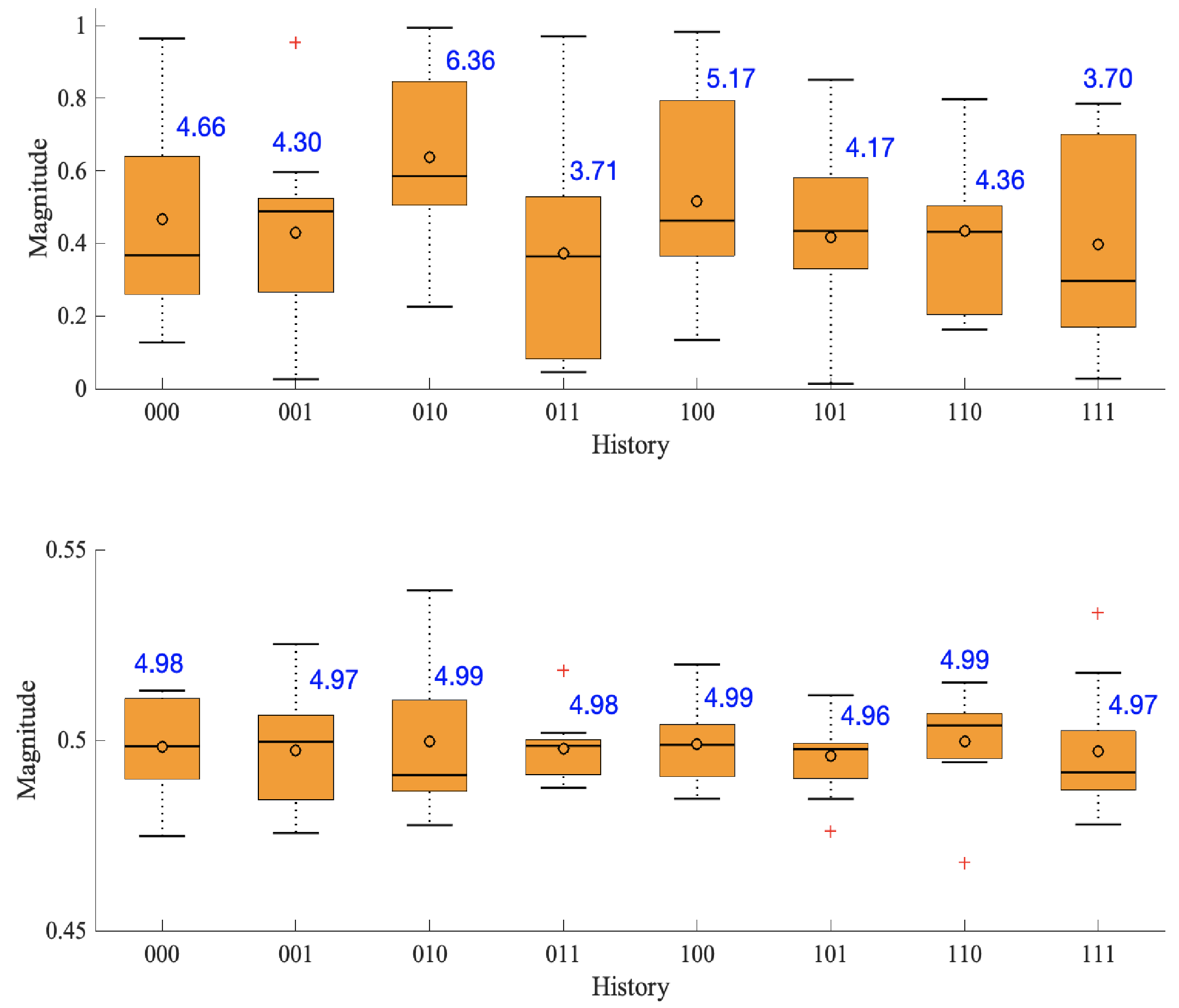
Figure 3 shows how the demands vary for each history index. The blue number next to each box give the demand total for the respective range of demands. Notice in the initial population there is a considerable variation of demands indicating almost no demand equity. Conversely, by generation 200 the mean of the demands are clustered around 0.5 which produces near optimal demand totals. There is also little variation indicating fair demand sets were found for every history index.

The 10 player game evolution had two uncoordinated rows in the initial population, one at generation 10 and none at generation 100. These simulation results suggest the evolutionary algorithm can find a coordinated demand matrix rather quickly. Intuitively finding a coordinated demand matrix should not be that hard since, by definition, it only has to have all coordinated rows—it does not require large demand totals in each row. Simulation results also indicate running the evolutionary algorithm longer will produce both higher row demand totals and fairer demands among the players. Although both attributes are important, it is perhaps more imperative to emphasize fair demands because it avoids exploitation. It is easy to determine the demand total, but how does one measure fairness?

Every demand $d_i\in (0,1]$. If rounded to the nearest cent, there are 100 non-zero demands a player can make and ${100}^n$ possible demand choices per round in an n-player game. Every row in the demand matrix can be considered a set of n samples with sample mean

$$\overline{d}=\frac{1}{n}\sum _{i=1}^n{d}_i$$

and standard deviation

$$\overline{s}=\sqrt{\frac{1}{n-1}\sum _{i=1}^n{(d_i-\overline{d})}^2}$$

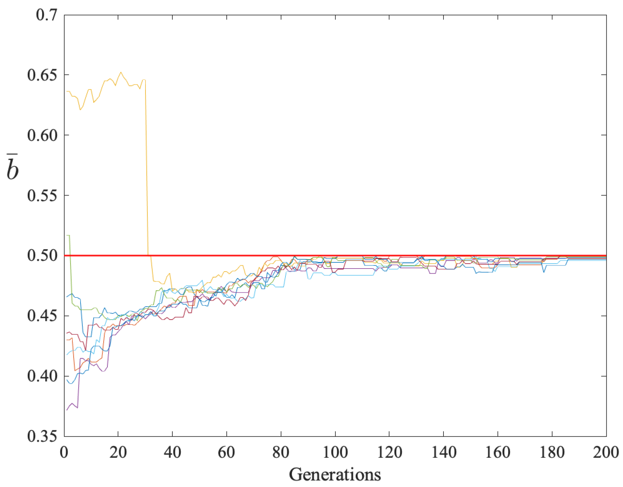
The optimal solution of an n-player GDD game is ${\left\{0.5\right\}}^n$ because the demand total is $n/2$ and with identical demands no player is exploited. The sample mean is an indicator of how close the bid total is to $n/2$. That is, $\sum d_i\to n/2$ as $\overline{d}\to 0.5$ from below3. A good demand matrix has $\overline{d}$ close to 0.5 in all rows so that the demand totals are near optimal regardless of the history profile.

Figure 4 shows the row sample means of the parent demand matrix versus generations. The row with history label ‘010’ had a sample mean above 0.6 for the first 32 generations before evolution produced a coordinated demand set. After 186 generations all rows converged with $\overline{d}\approx 0.498$.

The standard deviation in a row measures the spread of the demands around the sample mean. A small standard deviation means less spread. Thus, $\overline{s}$ can be used as an indicator of fairness. Empirical evidence suggests ${\overline{s}}_0=0.02$ is a reasonable upper bound for fair demand sets. Figure 5 shows how the row standard deviations changed during the evolutionary algorithm run. All rows had $\overline{s}<{\overline{s}}_0$ after generation 186.

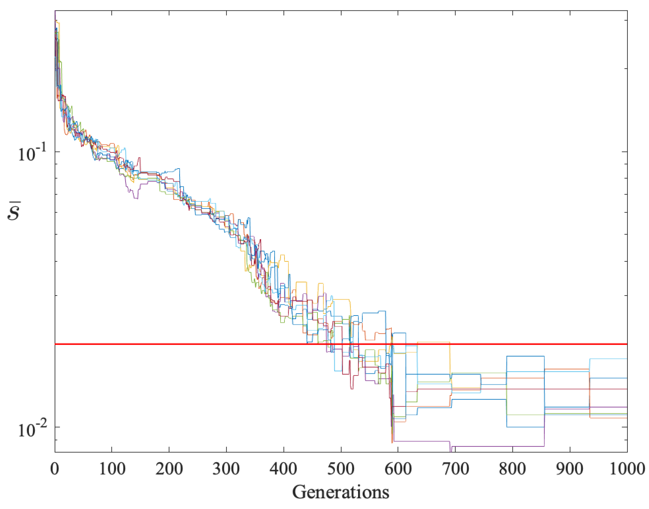
A 20-player GDD game was also simulated. Due to the larger number of players, ${\lambda }_n$ was increased to 18 and the run terminated after 1000 generations. Figure 6 and Figure 7 show the sample means and standard deviations respectively. After some initial variability, all rows converged to $\overline{d}\approx 0.499$ and $\overline{s}<{\overline{s}}_0$ after 690 generations.

MATLAB was used for all simulations and to plot the results.

6. Discussion

6.1. Evolving Player Sets

Evolutionary algorithms have been extensively used to find good players for n-player games. During each generation $\mu$ parents are perturbed to produce $\lambda$ offspring. The normal interpretation is each individual in the population is a separate player so $\mu =n$. Here a different approach was taken: every individual in the population is a set of n players.

The problem with evolving individual players is two-fold. First, it focuses the algorithm on the wrong objective. The highest fit individual in the population is usually just one player, not a set of n players. Even if the evolutionary algorithm uses elitism, where the best fit individual always survives, being highly fit in one generation may not carry over to future generations with different players (e.g., see [17,18,19]). A player’s opponents never change when they are evolved as a set, making the notion of fitness more meaningful. Second, the algorithm has to choose the best n players out of a pool of $\lambda >n$ offspring. A rather complex fitness calculation is required since it entails randomly picking multiple sets of n out of $\lambda$ individuals for evaluation. Treating each individual as a set of n players avoids doing that. The end result is a more computationally efficient fitness evaluation.

6.2. Demand Matrix as a Representation

Often one talks about an evolutionary algorithm exploring a fitness landscape but the move operator actually forces the algorithm to explore a search space $\mathbf{S}$. This search space consists of all genotypes that can be accessed from the initial population in a finite number of move operations. In discrete fitness landscapers—e.g., a binary string genome—it is straightforward to pick a move operator such that $\mathbf{S}\equiv \mathbf{G}$. However, if the genome is a real-value vector then the fitness landscape is continuous and $\mathbf{S}\subset \mathbf{G}$ if for no other reason than every vector component $x_i\in {\mathbb{R}}^k$ in the code has finite precision4.

Each column in the demand matrix constitutes a strategy vector for one of the players. A player only stores his assigned column. The vector components are labeled with a finite history index. A player selects a component with the appropriate history index as his demand in the next round. These demands may change during the evolutionary algorithm run which is analogous to a player trying different demands during a training session. Thus, the evolution can be thought of as emulating some underlying decision process.

There are two histories that can become fixed points. The vector component with index ‘000’ is a fixed point if that demand set is uncoordinated.

Table 6. History Trace.

History Index	History Trace
000	$000\to 001\to 011\to 111$
001	$001\to 011\to 111$
010	$010\to 101\to 011\to 111$
011	$011\to 111$
100	$100\to 001\to 011\to 111$
101	$101\to 011\to 111$
110	$110\to 101\to 011\to 111$
111	$111\to 111$

shows the history trace for each possible history state in a coordinated demand matrix; history ‘111’ is a fixed point in this case.

One might think with a coordinated demand matrix only the demand with history index ‘111’ need be kept since it is the only fixed point. Actually, the entire strategy vector should to be kept. Players do not know the demands of other players since the only feedback is the payoff (his demand if a coordinated demand set or zero payoff otherwise.) A player might be tempted to increase his demand to get a higher payoff if the population demands are at the ‘111’ fixed point. However, that demand increase might produce an uncoordinated set. In that case the history changes so keeping the entire strategy vector lets the player respond accordingly. The player can always reduce the increased demand to its original value to continue receiving positive payoffs.

6.3. Search Complexity

Each demand represents a coordinate of a point in ${\mathbb{R}}_{+}^n$. The $L_1$ norm of a vector from the origin to this point is the demand set total. The optimal demand total is $n/2$ dollars and every point with that $L_1$ vector norm forms a simplex. All points on or beneath the simplex surface represents a coordinated demand. Note that every point p in this coordinated subspace is a point in the search space $\mathbf{S}$ and therefore also a point in the fitness landscape $\mathbf{S}\cup \mathcal{F}$.

The optimum solution is all players demand 0.5, but that does not make the optimization problem trivial. Essentially you are trying to evolve an n-dimensional real vector with a small standard deviation among components and with an $L_1$ norm of $n/2$. The global optimum is at ${\left\{0.5\right\}}^n$. Seeing as there are multiple ways to split the surplus exactly, there are multiple local optima. In fact, every point on the simplex surface is a Nash equilibrium since any unilateral demand increase results in a zero payoff for all players. These Nash equilibria are not fitness equivalent.

Consider now a point in the coordinated subspace below the simplex surface. This point is not a Nash equilibrium because a player could, within limits, increase his demand and do better than the rest of the players. Such a point is not Pareto optimal either because a unilateral demand increase by one player does not necessarily decrease the payoff of any other player. The other players will still get their demand as a payoff so long as the $L_1$ norm is less than or equal to $n/2$. But even this region below the simplex surface has multiple local optima. Let $\gamma \in [0.00,0.01,\dots ,0.49]$ and assume all n players choose the same $\gamma$ for their demand. The point $p\in \mathbf{S}$ with coordinates $\left(\gamma ,\gamma ,\dots ,\gamma \right)$ is in the coordinated subspace below the simplex surface. The row fitness drops if any one player unilaterally changes his demand. Therefore, any point in the neighborhood of p has lower fitness, which makes p a local optimum.

Both $\overline{d}$ and $\overline{s}$ are needed to properly evaluate a set of n players. The demand total is $n\overline{d}$ and $\overline{s}$ measures fairness. Consider a 2-player game with demands (0.99, 0.01). The demand total $2\overline{d}=$$1 is optimal, but the demands are grossly unfair. Conversely, a game with demands (0.20, 0.19) is fair, but the demand total is well under $\$1$.

The genome described in this paper scales linearly with n, unlike the neural network approach. The neural network has $2n$ inputs and, assuming a hidden layer with one less node, $4n^2-1$ synaptic weights. Conversely, the proposed genome has only $8n$ parameters (demands) to evolve. In a 20-player game the neural network has nearly 1600 weights to evolve whereas the proposed genome has an order of magnitude less parameters to evolve. Due to these NN scaling problems, no comparison was made between the NN approach and the approach described in this paper.

6.4. Algorithm Termination

The $({\mu }_n+{\lambda }_n)$-ES uses a fixed number of generations as the termination criteria. One could instead terminate after the first generation that produced a coordinated demand matrix. But further evolution is likely to produce fairer demand sets with higher demand totals. Consequently, running a small number of generations after finding a coordinated demand matrix is recommended.

7. Summary & Future Work

This paper described an intuitive representation for GDD games with many players. The genome scales linearly with the number of players and a simple, efficient evolution strategy can find near optimal player sets regardless of the number of players. Unlike virtually all other evolutionary algorithms used to evolve game players, which evolves players one at a time, in this approach each move operation evolves an entire set of n players. The representation was used to successfully find players in 10 and 20 player GDD games.

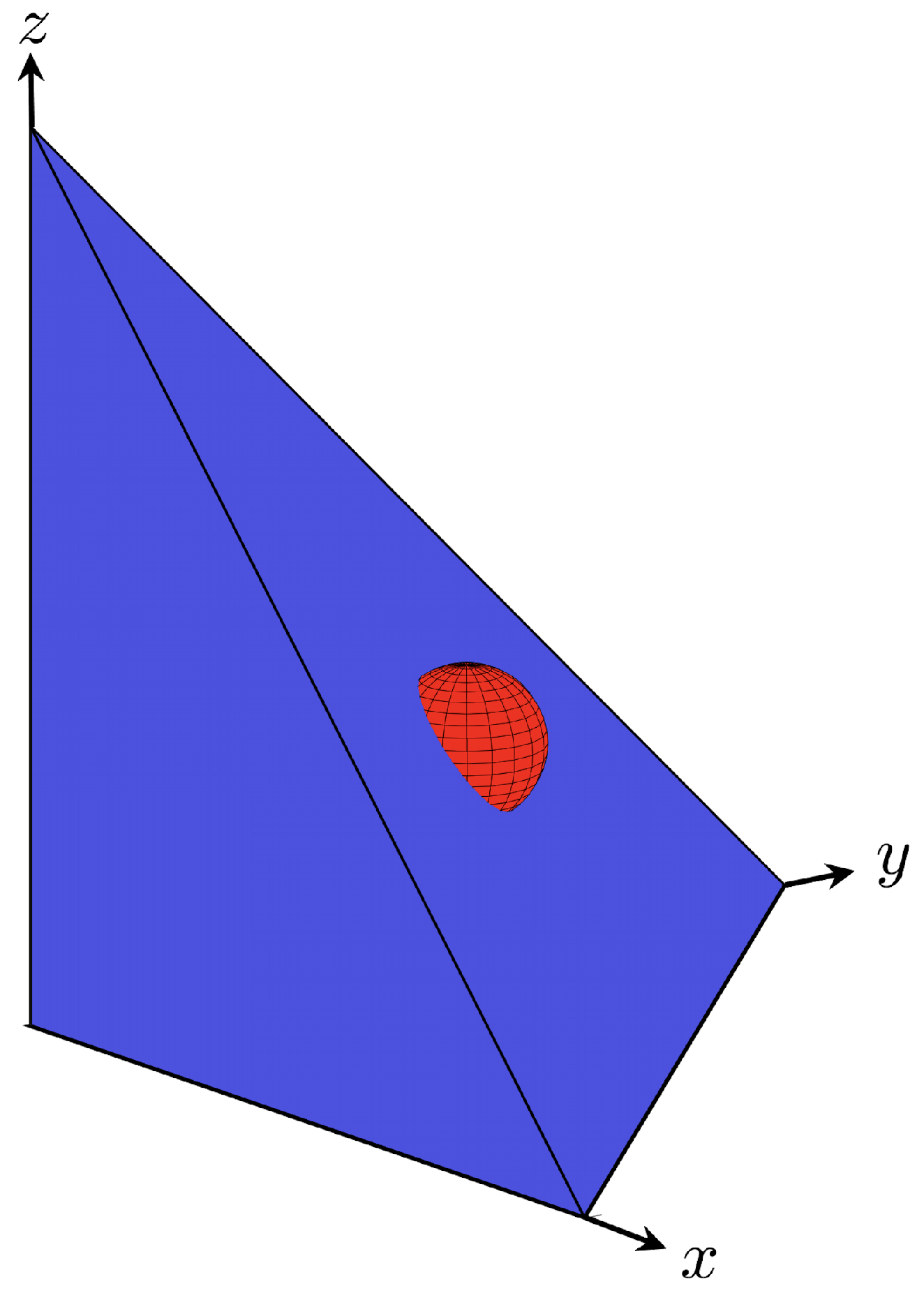
One of the interesting properties of the generalization of divide-the-dollar is that it permits a fairly complex game specification by simply specifying the scoring set. A GDD game can have subsidies [4], for example, through a simple modification of the scoring set. The idea is an additional amount is made available to encourage play near the fair ${\left\{0.5\right\}}^n$ range. This subsidy allows a players to receive a payoffs that sum more than $n/2$ if the players demands are within the area covered by the subsidy. An example of a subsidy for an $n=3$ game is shown in Figure 8. The hemisphere is centered at (0.5 0.5 0.5) and every point inside it is considered a coordinated demand. The subsidy generalizes smoothly to n players—an n-dimensional subsidy is added to the standard scoring set.

The generalization obtained by creating a subsidy by adding a hemisphere to the standard scoring set is one possible scoring set that has a clear meaning. In fact any subset of ${\mathbb{R}}^n$ can serve as a scoring set; it is important that the set have a meaning or interpretation. Sets with points that have negative coordinates might represent a model of money laundering, for example, though the parties supplying the money to be laundered would need a different objective score than other agent types.

In an earlier study [20] dynamic scoring sets were used in an $n=3$ agent version of GDD that studied the effect of having undependable subsidies—subsidies that are sometimes available and sometimes not, without warning. This study opens to door to studying scoring sets that can change between rounds of the game, modeling a stochastic scoring environment. The technique pioneered in this study for evolving a structure that specifies an entire cohort of players together may interact differently with dynamic payoff sets than co-evolved individual agents.

In general the outcome of evolving game playing agents is highly dependent on the agent’s representation. One obvious experiment would be to compare representations that permit co-evolution of individual agents (for an n-player game), with the jointly evolved agents presented in this study. The competitive advantage granted by each of the agent evolved strategies would be an interesting quality to assess. It would also be interesting to extend the demand matrix approach to other mathematical games. For example, a single fitness value reflecting fairness might affect the outcome of a tragedy-of-the-commons game. No limitations for finite population games are envisioned since each row of a demand matrix is an extension of a payoff matrix used in 2-player games.