Article

Groundwater Usage and Strategic Complements: Part I (Instrumental Variables)

1
Computational Social Science, Department of Humanities, Social and Political Sciences, ETH Zürich, 8050 Zürich, Switzerland
2
Behavioral Game Theory, Department of Humanities, Social and Political Sciences, ETH Zürich, 8050 Zürich, Switzerland
3
Institute of Sociology, University of Zürich, 8050 Zürich, Switzerland
*
Author to whom correspondence should be addressed.
Games 2022, 13(5), 67; https://doi.org/10.3390/g13050067
Submission received: 2 September 2022 / Revised: 10 October 2022 / Accepted: 13 October 2022 / Published: 15 October 2022

Abstract

:
We test whether the decisions in a common-pool resource game are better modeled game-theoretically as strategic substitutes or complements using an individual-level dataset of groundwater usage that accounts for 3% of US irrigated agriculture. Based on a regression framework with instrumental variables, we find support for strategic complements, suggesting that reciprocity– and/or race-to-depletion–like dynamics are key to understanding groundwater usage.
JEL Classification:
C72; Q12; Q20; Q25

1. Introduction

1.1. The Importance of Groundwater Usage

One of the biggest challenges facing the 21th century is sustaining common-pool resources (CPRs) and avoiding tragedies of the commons in the face of a growing global population and economy. Here are some facts from the report of the [1]: Global resource extraction has more than tripled since 1970, outpacing global population growth by 50%. During the first two decades of the third millennium, the growth rate in global resource extraction has matched the global GDP growth rate, and, looking forward, natural resource extraction is expected to double by 2050.
Of all the natural resources, groundwater—which is the focus of this paper—plays a key role in the sustenance of economic systems, and faces particularly serious depletion risks.1 More than 95% of usable and accessible freshwater is groundwater [6], and almost 80% of global agriculture relies on groundwater irrigation (see UNESCO reports from 2009 and 2012). The present rate of groundwater extraction, however, is unsustainable in basically every major groundwater basin in the world that is currently accessible (and not frozen). They have all been flagged as “depleting due to over-appropriation” [7] because of irrigation.
One particularly important groundwater system is the High Plains Aquifer system in the American Midwest, of which the Ogallala Formation is the best-known. Groundwater-usage in that region has been studied in economics since [8] (see also [9,10,11,12,13,14,15]). Nevertheless, relatively little is known about the behavioral aspects of the underlying CPR game played by the relevant humans accessing the common groundwater, in particular regarding the strategic nature of the underlying game. In this paper, we take water usage data from the this aquifer system in the Midwest as the basis, and test two competing hypothesis concerning the right game-theoretic modeling of groundwater use (and CPR games more generally) with focus on the question ‘Are groundwater use decisions strategic complements or substitutes?’
This is an important question, because if groundwater usage decisions are strategic substitutes then sustainable behavior incentivizes unsustainable behavior, and groundwater generally depletes. By contrast, if groundwater usage decisions are strategic complements then sustainable behavior incentivizes sustainable behavior, and unsustainable behavior incentivizes unsustainable behavior, and groundwater use can either be sustainable or turn into a race to depletion. Evidence on the matter from field experiments for CPR contexts that are not about common groundwater usage is mixed [16], for example, find that fishermen in their fishing decisions behave in a way that is “consistent with standard economic theory that assumes selfish preferences and non-cooperative behavior” (p. 413), mirroring what [17] found. By contrast, ref. [18] finds evidence from farmers with access to common forestries that “conditional cooperation and costly monitoring explain success in forest commons management” (p. 961).
Currently there is no empirical evidence based on observational groundwater data, hence our interest in this resource. The lack of such studies is likely owed to a lack of real-world data availability generally, as is argued by [19], and what is available lacks the detailed microscopic (individual-level) information necessary to test individual-level hypotheses. This is beginning to change as monitoring technologies have improved, and indeed this is what made our study possible, as the regions we study pioneer monitoring and measurement technologies for groundwater.
To date, comparable data was available almost exclusively for fishery contexts, where the amount of catch by individual boats has been recorded in some contexts for quite a while. Indeed, fisheries occupy a prominent place in the CPR literature, of which we shall mention only a few. The first CPR paper by [20] focused almost exclusively on fisheries (see Banzhaf et al. [21], who proposed a revealed preference test for Gordon’s model). The theory papers by [22,23] use fisheries as their main examples too, and fisheries have been the subject of many case studies [24], field experiments [17,25,26], framed field experiments [16], and artefactual field experiments [27]. Using large-scale observational data, ref. [28] “conduct the first empirical investigation of common-pool resource users’ dynamic and strategic behavior at the micro-level using real-world data”—and this data was from a North Carolina fishery. Today, also credit to the people who worked on this in the past, global fisheries are no longer amongst the most threatened CPRs. Based on the work of Ostrom and others, agreements have been reached that “have been successful in some 150 major fisheries of 170 species in seventeen countries ⋯ Since 1986, the system has been effective, largely eliminating overfishing, restoring stock to sustainable levels, and increasing fishermen’s profits,” (Stavins [29], p. 91).
Groundwater governance is clearly a pressing issue. As with fisheries, studying the micro-behavior underlying groundwater usage can help inform policy, particularly with focus on strategic complements/substitutes, because the two result in different policy recommendations. With strategic substitutes, ref. [30]’s view seems more plausible that only centralized authorities and private property institutions could sustain CPRs in the long-run. By contrast, with strategic complements and reciprocity-like behavior, ref. [31]’s advocacy for policies that foster self-governance, local norms, etc. seem promising alternatives.

1.2. Related Literatures

The CPR literature is well-known for case studies of the “Tragedy of the Commons” [20,30,32,33], whereby a population using a CPR for profit depletes the resource beyond what is collectively desirable. In the relevant theory literature, CPR interactions are typically modeled as dynamic-stochastic games à la [34], some with strategic complements, some with strategic substitutes, and some leaving it open. For some prominent examples, see [23,35,36,37,38,39,40,41,42,43,44,45,46,47]. Related experimental literature has identified reciprocity as a key driver of human behavior in these contexts, mechanisms of which include conditional cooperation [48], social preferences [49,50,51,52,53], interdependent preferences [54], interactive preferences [55,56], social pressuring [57,58], social norms [59,60,61], shared intentions [62], and collective identities [63,64]. Based on CPR case studies, ref. [31] identified reciprocity as emerging from local traditions, norms, values, social ties, etc. (see [65,66,67,68,69,70,71,72] for some of her most relevant work in this area, and [73] for an overview over Ostrom’s work and her perspective on game theory.

1.3. Our Contribution

In this paper, we test whether observational data supports a view of the CPR groundwater game with strategic complements or substitutes. We do so by analyzing a unique, individual-level dataset of groundwater-usage from Nebraska, US—which sits on top of one of the world’s largest groundwater reservoir systems—that accounts for three percent of US irrigated agriculture. (We view putting together and presenting the use case and dataset as a contribution in itself.) The dataset documents farmer-level groundwater pumping and includes a relatively rich set of control variables including land-size, soil quality, longitude-latitude coordinates, climate data, market data, as well as farmer-level information about whether groundwater recharges or depletes due to pumping. Importantly, this dataset describes farmer-level pumping in a policy-free area.
In this paper, we test the hypotheses using a procedure that has been successful in empirically analyzing networked panel data similar to ours building on recent work by [74], which promises consistency and robustness to endogeneity. Endogeneity is clearly a major issue in analyzing this issue, which is why this paper is only one part of two in our effort to use different methods in addressing this question. We refer the reader to our companion paper on the same topic, published alongside this paper, where we take a complementary revealed preference test route. In this paper, we pose the question of strategic substitutes versus complements by incorporating a strategic interaction term into a regression framework. This allows us to test for positive (or strategic complements) versus negative (or strategic substitutes) directly while controlling for a range of possibly confounding factors. Importantly, we allow the network that governs strategic interactions to be unknown, which allows us to leverage our latitude-longitude data to test behavior under a wide rage of possible mechanisms that could drive reciprocity-like behavior.
Our tests reject strategic substitutes in favor of strategic complements resoundingly. We reject strategic substitutes for different radiuses, neighborhood sizes, and under various regression specifications. While not immune to endogeneity issues, these results in combination with those from our companion paper, render the conclusions of this paper plausible.
As our title suggests, this is the first of two papers on the topic. Both papers investigate the strategic nature of gorundwater interactions using observational data. The approach of the present paper was discussed above. In our companion paper [75], our second of two papers on the topic, we tackle the same question–whether groundwater usage decisions are strategic substitutes or strategic complements–analyzing the same data from the Midwest as in this paper plus another data set from a different district using a different revealed preference testing approach. The two parts of the project come to the same qualitative conclusion that groundwater decisions are strategic complements, not strategic substitutes. There exists an earlier working paper version [76] containing prior (superseded) versions of both approaches. We have since split the paper in two and the present paper is one of the two paper superseding said working paper. We refer the interested reader to that earlier working paper version for some more detailed discussion of the dataset.

1.4. Structure of the Paper

The paper is structured as follows. In Section 2, we describe the various datasets used in our analyses. Section 3 presents the regression frameworks and outputs, the results of which we summarize in Section 4.
We also have two appendices. The estimation strategy for our regression framework is provided in detail in Appendix A. Robustness checks regarding the unterlying network are reported in Appendix B.

2. The Data

We study individual-level irrigation decisions from a district above the High Plains Aquifer (HPA) system, which is a system of more and less connected aquifers, of which the Ogallala is the best-known. Our district lies in Nebraska, US, and covers a largely self-contained pocket of an aquifer. This dataset is rich on an individual-level, which ultimately makes our tests possible. But before we describe the dataset itself, we would like to describe the context of the data in more detail. Readers less interested in context may read the summary only and skip the rest of this section.
  • Summary
In total, our final dataset consists of approximately 50,000 observations of farmer-level groundwater usage, as well as a rich set of controls concerning resource dynamics, farmer attributes, seasonal attributes, and market conditions. We summarize the datasets from 2008–2012 in Table 1, which are the years for which we were given data access. Our analyses is done in R.
  • Control variables

2.1. Groundwater in the American Midwest

Nebraska (the “Cornhusker State”) is one of the key contributors to US agriculture, being the number one red meat producer, second pinto bean producer, and third corn producer among the US states as per 2014 [77]. Nebraska’s agricultural productivity also competes on a global scale, being the twelfth largest player internationally in terms of irrigated land. Agriculture is the main economic activity in Nebraska with farm-related income contributing over $23 billion (24% of Nebraska GDP in 2013) and a quarter of jobs coming from agriculture.
Nebraskan agriculture crucially relies on freshwater from the HPA, which stretches across eight US states from southern South Dakota to northern Texas.2 Approximately 90% of groundwater pumped from the HPA is used to irrigate crops. But like most other aquifers around the world, the HPA is depleting due to over-pumping. Current estimates suggest that 15% of the aquifer has been depleted since the 1930s, and the current rate of depletion signals that further decline in groundwater levels is likely [78,79]. Nebraska, with nearly two-thirds of all the groundwater from the HPA, is particularly dependent on the HPA and particularly critical for its sustainability.3

2.2. Governing Groundwater: Nebraska’s Natural Resources Districts

Groundwater has been at the heart of policymaking in the American Midwest for a long time. But at first, policy makers struggled to incentivize farmers to pump groundwater because it was prohibitively costly to build and maintain irrigation wells. The first article in the first issue of the AER, “Some Unsettled Problems of Irrigation” [8], was dedicated to collective action problems associated with coordinating farmers to use irrigation technologies. However, the situation changed fundamentally in the 1960s with the invention of the center pivot irrigator, which made access to groundwater easier and cheaper. Groundwater depletion has become a problem since then, and in response, in 1969 the state of Nebraska founded 23 Natural Resources Districts (NRDs) to govern groundwater pumping. In fact, each district has full jurisdiction over governance of all natural resources within the district borders—which includes groundwater. Since then, the NRDs have adopted very different policies to govern groundwater pumping, and these differences play an important role in our empirical analysis below. Our data concern individual-level groundwater-usage behavior in one of the 23 NRDs, namely the “Upper Big Blue” NRD (UBB), which is the largest and most productive district in the state.
  • The “Upper Big Blue” District
The UBB is the largest and most irrigated district in Nebraska, alone accounting for 15% of Nebraska’s irrigated acres and 2% of the US’s irrigated acres. Given the size, it is perhaps surprising that this district takes a policy-free approach to regulating groundwater usage. Farmers pump groundwater without restrictions. The only regulatory measure taken by the UBB was requiring all farmers to install pumping meters on irrigation wells in 2006. This is why the dataset begins in 2007, and we have data through 2014.4

2.3. Empirical Regressors

Our empirical analysis utilizes data from different sources concerning (i) groundwater usage collected by the UBB, (ii) groundwater depletion, soil types and other controls collected by the University of Nebraska at Lincoln (UNL), (iii) market prices and land rental rates from the US Department of Agriculture,5 (iv)and rain and temperature from the US National Oceanic and Atmospheric Administration.6 Below, we categorize and describe the key variables pertinent to our study.
  • Farmer’s groundwater usage
Our ‘main’ datasets are the annual UBB records concerning farmer-level groundwater usage. For each of the roughly 10,000+ farmers in the UBB, we have data on total groundwater usage for each season from 2007–14, which amounts to nearly 100,000 observations. Data include (i) latitude-longitude coordinates of farmers’ farmland and (ii) the number of acres the groundwater serviced. We plot the spatial location of farmers in the UBB in Figure 1; black-white shading represents the average groundwater usage of each farmer (Figure 2).
  • Neighbors
Because the dataset includes latitude-longitude coordinates, we have the opportunity to account for the networked strategic interactions of groundwater usage. In other words, we have a way to control for with whom a farmer interacts strategically. There are three reasons we shall emphasize a farmer’s neighbors as those who play an important role in strategic interactions. First, neighbors are a natural starting point as farmers are more likely to observe, communicate and strategically interact in close proximity than with more distant farmers. Second, in line with Ostrom’s local governance principles, informal institutions—such as moral and social norms—operate on a local level. Third, there are so-called “local drawdown” effects [80,81,82] operating at the hydrological level. Local drawdown is caused by pumps drawing ‘local’ groundwater in close proximity first, which causes local depletion of neighbors’ groundwater-levels—season-long pumping gradually increases the set of neighbors on whom a farmer induces local drawdown. The hydrology literature typically defines a “radius of influence” in which local drawdown is measurable by the end of the farming season, which ranges from 200ft to a mile [83].
  • Groundwater dynamics
The HPA is a so-called “water table aquifer” because there exists a clear “upper-boundary” of the aquifer—often referred to as the water table level—that moves closer to the surface-level if the resource is recharging and further away if the resource is depleting [84,85]. We follow geologists, hydrologists and government officials in using water tables as proxies for depletion risks. Researchers at UNL kindly provided us with relevant data for UBB for our years of interest.7 The data include measurements at more than 500 locations in the UBB, time-stamped as Spring or Fall, which allows us to empirically track groundwater depletion within season, as well as resource recharge between seasons. Based on this data, we use standard spatial interpolation methods to estimate groundwater levels in the Spring and Fall of every season at every location in the dataset.8
The UNL dataset also records depths of wells, and we use the same spatial interpolation method noted above to estimate the well depth for each farmer.9 Other, separate datasets from the UNL allow us to use similar procedures to obtain controls for transmissivity10 and soil types. We add to these datasets by including seasonal rain and temperature (sum and average from April to September, respectively) from data by the US National Oceanic and Atmospheric Administration. Finally, we include three market variables from the US Department of Agriculture: (i) average spot market price of corn from 1 April to 1 October of each season (we focus on corn because, in a typical year, roughly 70% of irrigated land is for corn), (ii) average price of electricity between April and October, and (iii) farmland rental rates which are available averaged at the county level each season (there are nine counties in the UBB).

3. Estimating Strategic Interactions

3.1. Regression Setup

  • Strategic network
The first step in estimating strategic interactions is clarifying with whom a farmer strategically interacts. To do so, the longitude-latitude information in the dataset comes into play. Let N i N \ { i } be the set of farmer i’s neighbors, a subset of the set of all farmers N . We combine neighborhoods to define a strategic network A R + N × N as a N-by-N matrix where each row A i = ( A i j ) j N represents farmer i’s neighborhood such that A i j > 0 if and only if j N i , and A i j = 0 otherwise. The matrix is row-normalized.
  • Regression Model
Suppose that the strategic network, A , is known a priori (we relax this assumption later on). We assume that farmer i’s behavior in season t T is explained by11
w i t = α i + β N j N A i j w j t + X i t ψ + y t ϕ + d i γ + u ˜ i t .
The second term, β N j N A i j w j t , corresponds to i’s behavior as determined by strategic interactions. X i t denotes a 1 × K vector of individual-level time-varying exogenous controls included in the dataset—including groundwater levels and interaction terms, such as rain t × land-size i —and ψ is the corresponding K × 1 parameter vector. y t denotes a 1 × L vector of UBB-wide time-varying exogenous controls included in the dataset—including crop prices, electricity prices, rain, temperature, and land rental rates—and ϕ is the corresponding L × 1 parameter vector. d i is a 1 × R vector of farmer-level time-invariant controls—including land-size, well depth, transmissivity, and soil type—and γ is its corresponding R × 1 parameter vector. α i is a farmer specific fixed-effect constant. Because we are interested in β N , we can use a first-difference estimator, which means that we estimate
w i t w i t 1 = β N j N A i j w j t w j t 1 + X i t X i t 1 ψ + y t y t 1 ϕ + u i t ,
thereby avoid estimating ( α i ) i N and γ .
The final term, u ˜ i t , captures overall disturbance and makes it possible to control for unobserved and possibly confounding factors. Perhaps most importantly, we must control for disturbances that can occur spatially; e.g., hail storms can damage a localized region of the UBB, which is unobserved in the dataset but may appear to take the form of positive/negative strategic interactions between farmers. We can model such unobserved events by exploiting the fact that it changes behavior in a spatially tractable way.
We proceed with a commonly made assumption that such disturbances are related via a first-order spatial autocorrelation expression, which is given as
u i t = ρ j N B i j u j t + ν i t .
where ρ is the degree of spatial correlation, B R + N × N is a weighting matrix that governs the spatial relation between i and j ( B may be different than A ), and ν i t captures the individual-time innovations. The expression in (3) is also known as a [89,90] process (see also [74,91,92]). The interpretation of (3) is that, if j receives an unobserved shock u j t , then his/her neighbors defined by B experience a shock ρ u j t .
Our goal is to estimate (2) and (3).
  • Hypotheses
Based on the regression setup above, our null and alternative hypotheses are given as follows.
Null hypothesis,  H 0 : Framers’ groundwater-usage decisions are strategic substitutes or do not exhibit any systematic relations.
Alternative hypothesis,  H A : Framers’ groundwater-usage decisions are strategic complements.
Note that the competing hypotheses are set up to be slightly asymmetric as we pool the cases of strategic substitutes and of unsystematic relations in the null hypothesis, with the alternative hypothesis being only strategic complements. We do so in order to set up the analysis ‘against’ strategic complements and to give the benefit of the doubt to strategic substitutes by allowing for the possibility that, in our regression framework, strategic substitutes are not identifiable.
How do H 0 and H A translate to the regression setup above? Supposing we estimate (2) and (3) robustly, we consider effects with β N + 2 SE < 0 to represent strategic substitutes, effects with β N [ 2 SE , 2 SE ] to represent weak or unsystematic relations, and effects with β N 2 SE > 0 to represent strategic complements. Hence, H 0 predicts β N 2 SE 0 , while β N 2 SE > 0 supports H A ). In order to reject H 0 , we must therefore observe estimates of β N that are significantly positive and larger than 2 SE . Before discussing the p-value associated with testing H 0 vs. H A , we must first discuss how we estimate (2) and (3).

3.2. Identification

As we briefly noted in the introduction, such a regression model cannot be estimated without somehow addressing issues related to endogeneity. In particular, if water j t is used to explain water i t , which is used to explain water j t , then there exists endogeneity that may bias the estimation of coefficients in uninterpretable ways—as j influences him/herself by virtue of influencing i. This identification issue is known as the reflection problem [93,94], and resolving it requires a suitably selected set of instrumental variables (IVs).12
We address this issue by utilizing an IV setup proposed by [74] for fixed-effect regression designs (which builds on [91,92]). Specifcially, ref. [74] assume that, from any farmer i’s perspective, his/her neighbors’ control variables do not influence w i t directly, but only indirectly by virtue of influencing j N A i j w j t  directly. This means that A and i’s neighbors’ control variables can be used as the basis of IVs. [74] go on to show that B can be used to render such IVs uncorrelated with the error terms, which means that β N is identified in our setting.
Following [74], A , B and the control variables in the dataset can be organized to form IVs for estimating (2) and (3). We refer the interested reader to Appendix A for a derivation of the IVs as well as a discussion on the assumptions required to estimate (2) and (3) robustly. It should be noted that ours is an attempt to deal with endogeneity, but some spatial correlations will likely affect our analysis in a way that precludes an entirely robust effort.

3.3. Testing Procedure

The estimator procedure proposed by [74] requires an assumption that is somewhat problematic in our setting, namely that matrices A and B are observed. Our setting has a different setup. The UBB dataset has information about the geographical location of farmers, and it is possible to leverage this information to define a network that represents interactions based on local drawdown. Yet, while we have reason to believe that defining ‘local’ interaction networks based on this information is a reasonable starting point, such a network may not necessarily represent the true strategic interaction networks describing reality.
It turns out that resolving this issue also allows us to derive a p-value for testing our hypotheses. We proceed as follows. We define a set of networks N large enough to encompass at least one A * , B * N that represent the true network of strategic interactions and spatially correlated disturbances, respectively. We then randomly sample from this set of networks and estimate (1) and (3), which means that we recover β N ± 2 SE from each randomly sampled network. Perhaps somewhat surprisingly, it is shown below that the ‘sampling’ of β N s in this way follows a normal distribution (statistically speaking). This allows us to calculate the probability of identifying a network such that β N 2 SE 0 , which is given as
P A , B N : β N 2 SE 0 .
Recall that, for an estimated β N ± 2 SE , β N 2 SE 0 according to H 0 . This means that (4)—which is the probability of sampling such that H 0 is true—serves as a p-value for testing H 0 versus H A .
This testing procedure is valid only if the true networks A * and B * are inside of N . More formally, we say that N R + N × N is the set of feasible networks if it contains every A R + N × N such that: (i) A i i = 0 , or no farmer strategically affects him/herself, (ii) A i j > 0 only if i and j are less than 5 miles apart, depending on the case, (that is, only neighbors induce strategic interaction effects), (iii) A i j = A i k for any j and k with non-zero weights, or neighbors strategically affect i equally, and (iv) A is row normalized. Our testing procedure requires the following assumption.
Assumption A1.
Let N represent the set of feasible networks. Then there exists at least one pair of networks A * , B * N that represents the true network of strategic interactions and spatially correlated disturbances in the UBB, respectively.
We assume that neighbors come from less than 5 miles for two reasons. First, we incorporate the ‘local drawdown network’, which characterizes interactions that occur between farmers less than 1 mile. Second, we wish to extend the network space in order to incorporate other possible avenues for strategic interactions. It could be that the true network of interactions takes place on a larger scale than one mile if, e.g., mechanisms such as social pressure are at play—this is especially true taking into account that some farmers live in towns that are several miles away from their farm land. Therefore, we increase the scope of possible networked strategic interactions to increase the scope of possible mechanisms that could be tested.
In Appendix B, we run the same statistical test supposing that networked strategic interactions take place between farmers less than { 1 , 3 , 10 , 20 } miles away as a robustness check. We find that the results are qualitatively the same as those presented below.

3.4. Results

We randomly sample 10,000 pairs of A , B N and estimate (2) and (3) for each pair accordingly. This allows us to estimate (4), namely the probability of sampling a network that supports our null hypothesis that farmers’ decisions are strategic substitutes.
But before we can discuss these results, it is crucial to understand whether we have ‘good’ IVs. [74] prove that the IVs—which we derive in Appendix A—are orthogonal to the disturbances terms. While this is important, the IVs must still be sufficiently correlated with w N i t for the purposes of identification. A number of issues can arise if we do not have ‘good’ IVs: if we have weak IVs or if the results are sensitive to which IVs are used, then any findings we report are potentially moot. We thus show evidence that our IVs are valid before discussing the main findings.
  • Robustness of IVs and Consistency
One way to check IVs is testing whether results are robust to different IVs. With a number of different IVs, if each report a different strategic interaction term β N , then we are left with a problem because it suggests that our IVs are either (i) weak or (ii) unable to identify w N i t robustly. Yet, if different IVs each yield roughly the same β N , then we have good reason to believe that our IVs are indeed identifying strategic interactions.
We take this approach as a robustness check of our IV estimation procedure. We estimate (2) and (3) using six different IV setups, and we report the findings in Table 2. The first two focus on using groundwater levels and UBB-wide variables, such as rainfall and crop prices. The second two models focus on using individual-level and UBB-wide variables, such as (land-size i )×(rainfall t ). The fifth model utilizes a mix of IVs from the previous four. The final model utilizes all control variables included in our UBB dataset. To estimate parameters, we randomly sample 10,000 networks A , B N and combine the regression estimations using Rubin’s rule [98]. This means that: (i) the coefficients are combined using a simple average, (ii) standard errors are combined in a way that accounts for between- and within-variance of the estimated coefficients, and (iii) p-values are computed using the Barnard-Rubin corrected degrees of freedom [99]. All coefficients are normalized, so that, for all the control variables, β = % increase in groundwater usage per + 1 SD increase in the variable.
Two patterns in Table 2 give positive evidence that our UBB control variables are able to identify strategic interaction effects. First, in models (2,4,6) where we include market and climate trends, we recover roughly the same β N . Interestingly, model (3) shows that interacting farmer-level controls with climate variable also results in the same β N as models (2,4,6) but with very high SEs. The interpretation is that the IVs in model (3) were consistent but very weak. Second, it is obvious when IVs are weak/fail in Table 2. Models (1) and (5) show that when market and climate variables are excluded, we recover estimates where β N 1 . This is problematic because spatial regression models are generally not identifiable if β N 1 , and recovering β N 1 suggests that identification issues are present.
The main takeaway is that our estimation procedure is robust to which IVs we use, as long as we use ‘good’ IVs. As such, we proceed with model (6) because it yielded the lowest SE for β N . Our main findings do not change if we instead use model (2) or (4).
As concerns consistency of our estimators, we observe empirically that β N converge to the reported value after 1000–2000 random samples every time we repeat the empirical experiment. This is the case for our main setup whereby networks are selected independently and uniformly at random (with replacement) from the set of all restricted networks as per Assumption 1, we well as for other ‘neighborhood’ constructions (as reported in Appendix B).

4. Summary of Results

Our main findings, presented in Figure 3 and Figure 4, are based on the 10,000 regressions that underlie model (6) in Table 2. First, in the figure, we plot every ( β N 2 SE ) estimated for each randomly sampled A , B N ; in practice, there are 10,000 estimates. The visual evidence is unambiguous: we find that every estimated β N 2 SE > 0.2 > 0 . This already points to strong and robust evidence against no strategic interaction or strategic substitutes. The table confirms the visual impressions of the histogram. We find that the distribution of recovered β N 2 SE follow a normal distribution—we report the fitted normal distribution in the fist column, N ( μ , σ 2 ) , and the Kolmogorov-Smirnov test p-value in the second column ( p = 0.70 ). With evidence of β N 2 SE following a normal distribution, we can thus estimate the probability of drawing any A , B N such that β N 2 SE 0 , which serves as the p-value for testing H 0 vs. H A (see Equation (4)). We report this value in the third column, and as is visually evident in the histogram too, the probability of finding networks such that β N 2 SE 0 is statistically negligible. This means that we reject the null hypothesis with unambiguously low p-values.
Our results therefore provide evidence in favor of strategic complements. Indeed, it is clear from model (6) in Table A2 that the strategic interaction terms are the main drivers of behavior. Therefore, strategic complements not only characterizes behavior better than strategic substitutes, but it also characterizes behavior better than models that do not take strategic interactions into account. The other factors explain poorly in comparison. In particular, crop price movements have a minor a effect on groundwater-usage. Rainfall is the second strongest predictor of behavior, where we find that a 1 SD increase in rainfall ( = 5.8 inches) is associated with a 16% decrease in groundwater usage. Farmland rental rates is also strongly associated with groundwater-usage (which complements [100]). We find that β N is greater than 2 × the absolute value of any other effect, and, on average, a 50% decrease in neighbors’ pumping is associated with a 13.7% decrease in a farmer’s pumping.
Our conclusions are robust to other network assumptions. The testing procedure we presented above assumed that neighbors are other farmers less than five miles away. In Appendix B.2, we relax this assumption by running the same testing procedure and allowing that neighbors can be { 1 , 3 , 5 , 10 , 20 } miles away. We report p-values for each case in Table A1 and combine the 10,000 regressions for each case via Rubin’s rule in Table A2. We find that, qualitatively, our results remain unchanged: β N 2 SE > 0 for every A , B N we randomly sample. For every model, we unambiguously reject our null hypothesis in favor of strategic complements characterizing groundwater pumping interactions.
The test procedure in this paper was based on a regression framework with instrumental variables. Our companion paper [75] performs revealed preference tests for a class of dynamic CPR games. Both papers come to the same conclusion that groundwater usages are strategic complements.

Author Contributions

Conceptualization, C.M.K.; Data curation, C.M.K.; Formal analysis, C.M.K.; Methodology, C.M.K.; Supervision, H.H.N.; Writing-original draft, C.M.K. and H.H.N.; Writing—review and editing, C.M.K. and H.H.N. All authors have read and agreed to the published version of the manuscript.

Funding

This research was partly funded by the E.R.C. Advanced Investigator Grant “Momentum” for both C.M.K. and H.H.N., H.H.N. is currently funded by the Swiss National Foundation under Eccellenza “Markets and Norms”.

Data Availability Statement

The data belongs to the relevant Natural Resources Districts. Please contact the corresponding author for data requests.

Acknowledgments

We thank Rahul Deb, Rod DeBuhr, Andreas Diekmann, Dana Divine, Stefano Duca, Julia Franck, Philip Grech, Dirk Helbing, Barbara Ikica, Nate Jenkins, Yuichi Kitamura, Marie Krausnick, Jonathan Newton, Bary Pradelski, John Quah, Tatsuyoshi (Yoshi) Saijo, Larry Samuelson, Koji Shirai, Scott Snell, Aaron Young and Peyton Young for their support and comments, as well as anonymous editors and referees, and seminar participants at ETH Zürich, University of Zürich, KAUST, University of Oxford and Stony Brook University. All views expressed herein are ours and do not necessarily reflect the views of others, in particular, the Upper Big Blue District or the Nebraska Department of Natural Resources Districts. Any remaining mistakes are our own.

Conflicts of Interest

The authors declare no conflict of interest.

Appendix A. Instrumental Variables

In order to estimate (1) and (3) robustly, we rely on the following assumptions (for notation: I N is the N-by-N identity matrix).
Assumption A2.
In the regression model (1) and (3):
(A1.1) 
The individual-time innovations ( ν i t ) ( i , t ) N × T are i.i.d. with finite absolute 4 + δ ν moments for some δ ν > 0 . Furthermore, E [ ν i t ] = 0 and E [ ( ν i t ) 2 ] = σ ν 2 > 0 .
(A1.2) 
The matrices ( I N β N A ) and ( I N ρ B ) are non-singular.
Assumption (A1.1) ensures that individual innovations are well-behaved. Assumption (A1.2) is a mild condition in our setting and ensures that the matrix of strategic interactions is also well-behaved for estimation purposes. See [74,91,92,97] who also make such assumptions.

Appendix A.1. Derivation of IVs

Ref. [74] derived the ideal set of IVs for estimating (2) and (3). To present and discuss these IVs, we require additional notation. Stack groundwater usage in the following way:
w = w 1 1 , w 2 1 , , w N 1 , w 1 2 , , w N 1 T , w N T
We can write the regression model compactly by stacking the explanatory and control variables accordingly:
w = I N T α + β N A w + X Ψ + D γ + u u = ρ B u + ν
where I N T is an identify matrix of size ( N · T ) × ( N · T ) . Denoting ι T as a vector of ones of length T and ⊗ as the Kronecker product: A = I T A is the stacked strategic network, D = ι T D is the stacked individual controls matrix, and B = I T B is the stacked disturbance matrix. The remaining variables—namely α , X , γ , u , and ν —are ordered as w . Note that X collects both X i t and y t terms, and Ψ collects ( ψ , ϕ ) .
Next, we introduce a standard within transformation matrix to normalize (A1) (see, e.g., [92,101]). To this end, let J T be a T × T matrix of unit elements. We define Q 0 = I T 1 T J T I N as the standard within transformation matrix such that, for any matrix A of size ( N · T ) × ( N · T ) , Q 0 A results in a matrix such that the mean of every row is zero:
Q 0 A k l = A k l 1 N · T l = 1 N · T A k l .
It follows that
Q 0 w = β N Q 0 A w + Q 0 X β + Q 0 u Q 0 u = ρ Q 0 B u + Q 0 ν
where Q 0 removes time-invariant elements including α and D . This equation is what we ultimately estimate, since it retains the key variable of interest, β N , with fewer terms to handle.
Ref. [74] show that the ideal set of IVs for estimating (A2) is given by Q 0 G 0 where G 0 contains a subset of linearly independent columns of
X , A X , A 2 X , , B X , B A X , B A 2 X , .
The interpretation is as follows. Consider i’s neighbors, N i . X represents i’s individual attributes; A X represents i’s neighbors’ attributes; A 2 X represents i’s neighbors’ neighbors’ attributes; etc. Each are exogenous from the perspective of farmer i. In addition, because behaviors are assumed to be networked: X explains i’s behavior, which in turn influences N i ’s behavior; A X explains N i ’s behavior; A 2 X explains N i ’s neighbors’ behavior, which in turn influences N i ’s behavior, etc. Put another way, the network itself allows us to use farmers’ attributes as exogenous IVs to explain behavior in different parts of the network.
With Assumption A2 and an additional asymptotic assumption common in the spatial panel data literature,13 the estimation procedure proposed by [74] is consistent and asymptotically normal (we refer the interested to details therein). We follow this procedure to formulate our results in the main text.

Appendix B. Robustness Checks

Appendix B.2. Strategic Interactions on Different Network Structures
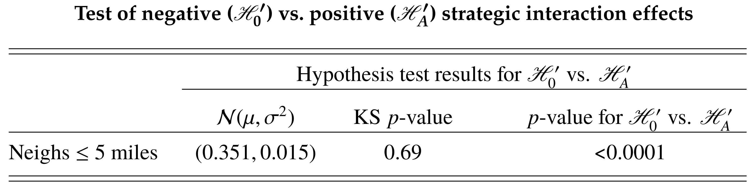
In Section 3, we estimated strategic interaction by assuming that neighbors were less than 5 miles away. In this section, we explore what happens when we weaken (strengthen) the ‘5 mile’ assumption by increasing (decreasing) this distance. We suppose that neighbors may come from less than { 1 , 3 , 10 , 20 } miles away. { 1 , 3 } are distances that get closer to the local drawdown networks. { 10 , 20 } considerably increase the space of possible network configurations, thereby increasing the likelihood of drawing networks that are consistent with strategic substitutes. For each case, we utilize the same test procedure as outlined in Section 3.
Table A1. Hypothesis test results for H 0 vs. H A .
Hypothesis Test Results for H 0 vs. H A
N ( μ , σ 2 ) KS p-Valuep-Value for H 0 vs. H A
Neighs ≤ 1 mile ( 0.072 , 0.009 ) 0.70<0.001
Neighs ≤ 3 miles ( 0.234 , 0.014 ) 0.70<0.001
Neighs ≤ 5 miles ( 0.351 , 0.015 ) 0.70<0.001
Neighs ≤ 10 miles ( 0.434 , 0.013 ) 0.69<0.001
Neighs ≤ 20 miles ( 0.29 , 0.009 ) 0.69<0.001
We report results in Table A1 (we re-report the 5 miles case for the sake of comparison). This table shows that the results reported in the main text are robust to different ways of defining neighborhoods. Firstly, as in the 5 mile case, we evidence that the distribution of β N 2 SE < 0 follows a normal distribution. Secondly, for each case { 1 , 3 , 10 , 20 } , we find that the probability of drawing networks that result in negative strategic interactions (or β N 2 SE < 0 ) is statistically negligible. This means that we reject the null hypothesis H 0 based on strong evidence for positive strategic interactions.
In Table A2, we also report the aggregated results of each regression. As in the 5 mile case, we find that strategic interactions is the strongest predictor of groundwater-usage.
Table A2. Micro-level regressions on UBB data. Number of observations = 97,160. { 1 , 3 , 5 , 10 , 20 } mile(s) corresponds to neighborhood sizes as in Figure 4. Coefficients of control variables are normalized such that β = % water i t /+1SD variable.
Dependent Variable: Log (Water i t )
(1 Mile)(3 Miles)(5 Miles)(10 Miles)(20 Miles)
Strategic interaction effects
 Log(Neighbors’ water i t )0.095 ***0.271 ***0.395 ***0.483 ***0.339 ***
(0.015)(0.023)(0.027)(0.027)(0.026)
Groundwater controls
 Spring GW i t −0.063 ***−0.059 ***−0.057 ***−0.055 ***−0.053 ***
(0.006)(0.006)(0.006)(0.006)(0.006)
 Spring GW i t − Fall GW i t 1 0.059 ***0.055 ***0.051 ***0.047 ***0.045 ***
(0.003)(0.003)(0.003)(0.003)(0.004)
UBB-wide time-level controls
 Spot market price t 0.027 ***0.02 ***0.016 ***0.014 ***0.024 ***
(0.003)(0.003)(0.003)(0.003)(0.004)
 Electricity t −0.172 ***−0.137 ***−0.112 ***−0.095 ***−0.126 ***
(0.007)(0.008)(0.009)(0.009)(0.012)
 Land rental rates i t 0.16 ***0.129 ***0.107 ***0.09 ***0.102 ***
(0.004)(0.005)(0.005)(0.006)(0.006)
 Rain t −0.242 ***−0.196 ***−0.163 ***−0.141 ***−0.182 ***
(0.005)(0.007)(0.008)(0.008)(0.008)
 Temperature t −0.156 ***−0.124 ***−0.102 ***−0.088 ***−0.122 ***
(0.006)(0.007)(0.007)(0.008)(0.01)
Farmer-level and time-level controls
 (Temp.) × (Rain) t −0.078 ***−0.065 ***−0.055 ***−0.049 ***−0.069 ***
(0.004)(0.004)(0.005)(0.005)(0.007)
 (Land-size) × (Rain) i t −0.017 ***−0.017 ***−0.017 ***−0.017 ***−0.017 ***
(0.002)(0.002)(0.002)(0.002)(0.002)
 (Land-size) × (Temp.) i t −0.012 ***−0.012 ***−0.012 ***−0.012 ***−0.012 ***
(0.002)(0.002)(0.002)(0.002)(0.002)
 (Well depth) × (Rain) i t −0.011 ***−0.011 ***−0.01 ***−0.009 ***−0.009 ***
(0.002)(0.002)(0.002)(0.002)(0.002)
 (Well depth) × (Temp.) i t 0.006 **0.006 **0.005 **0.006 **0.006 **
(0.002)(0.002)(0.002)(0.002)(0.002)
 (Land-size) × (Rain) × (Temp.) i t −0.016 ***−0.016 ***−0.016 ***−0.016 ***−0.016 ***
(0.002)(0.002)(0.002)(0.002)(0.002)
 (Well depth) × (Rain) × (Temp.) i t −0.019 ***−0.018 ***−0.018 ***−0.017 ***−0.017 ***
(0.002)(0.002)(0.002)(0.002)(0.002)
Note: ** p < 0.01; *** p < 0.001

Notes

1
Groundwater depletion is also connected with other major problems such as climate change [2,3] and rising sea levels [4,5].
2
To give an idea of its size: if spread across the US, the HPA would cover all fifty states with 1.5 ft of water (https://www.scientificamerican.com/article/the-ogallala-aquifer/ (access on 7 January 2022)).
3
The HPA is considered a renewable CPR in Nebraska, since snowmelt from the Rocky Mountains and annual rainfall are, with moderate levels of pumping, sufficient to sustain groundwater levels.
4
We would like to cordially thank Rod DeBuhr, Marie Krausnick, and Scott Snell at the UBB for permission and access to UBB data, as well as conversations that have greatly contributed to our study.
5
6
https://www.noaa.gov (access on 1 September 2022)
7
We are grateful to Dana Divine and Aaron Young for helping us include this data in our analyses.
8
More specifically, we utilize a method called “kriging”; see [86,87] for the seminal texts and [88] for a modern treatment. Under reasonable assumptions, this method provides the best linear unbiased prediction of geo-spatial intermediate values that maintains geologically relevant properties, such as continuity of the water table.
9
Note that well depth despite the active decision to drill a well is not per se a choice variable, because wells are drilled as deep as needed to get to the groundwater.
10
Transmissivity is a metric for how fast groundwater moves across the groundwater basin. Importantly, as a farmer irrigates, higher transmissivity implies the basin ‘replaces’ faster and alleviates the stress on water table levels during pumping, which helps stabilizes groundwater levels. Hence, farmers with higher transmissivity are less prone to receding water table levels.
11
When implementing this regression, we work with log w i t rather than w i t since w i t < 0 is not possible. We remove log to keep notation lighter.
12
See [95] for an overview of the reflection problems and various approaches to resolving it. In spatial/network games à la [96], using IVs is one of the most systematically explored means of resolving endogeneity; see, e.g., [97]. We utilize a technique proposed by [74] because it allows us to incorporate spatially correlated errors.
13
In particular, we require Assumption 3.3 from [74]. Other versions of this assumption can be found in [91,102,103].

References

  1. International Resource Panel (IRP). Groundwater Resources Outlook 2019: Natural Resources for the Future We Want; Technical Report; United Nations Environment Programme: Nairobi, Kenya, 2019. [Google Scholar]
  2. Green, T.R.; Taniguchi, M.; Kooi, H.; Gurdak, J.J.; Allen, D.M.; Hiscock, K.M.; Treidel, H.; Aureli, A. Beneath the surface of global change: Impacts of climate change on groundwater. J. Hydrol. 2011, 405, 532–560. [Google Scholar] [CrossRef] [Green Version]
  3. Taylor, R.G.; Scanlon, B.; Doell, P.; Rodell, M.; Van Beek, R.; Wada, Y.; Longuevergne, L.; Leblanc, M.; Famiglietti, J.S.; Edmunds, M.; et al. Ground water and climate change. Nat. Clim. Chang. 2013, 3, 322. [Google Scholar] [CrossRef] [Green Version]
  4. Konikow, L.F. Contribution of global groundwater depletion since 1900 to sea-level rise. Geophys. Res. Lett. 2011, 38, L17401. [Google Scholar] [CrossRef] [Green Version]
  5. Wada, Y.; Beek, L.P.; Sperna Weiland, F.C.; Chao, B.F.; Wu, Y.H.; Bierkens, M.F. Past and future contribution of global groundwater depletion to sea-level rise. Geophys. Res. Lett. 2012, 39, L09402. [Google Scholar] [CrossRef] [Green Version]
  6. Gleick, P.; Palaniappan, M. Peak water limits to freshwater withdrawal and use. Proc. Natl. Acad. Sci. USA 2010, 107, 11155–11162. [Google Scholar] [CrossRef] [Green Version]
  7. Gleeson, T.; Wada, Y.; Bierkens, M.F.; van Beek, L.P. Water balance of global aquifers revealed by groundwater footprint. Nature 2012, 488, 197–200. [Google Scholar] [CrossRef] [PubMed]
  8. Coman, K. Some unsettled problems of irrigation. Am. Econ. Rev. 1911, 1, 1–19. [Google Scholar] [CrossRef]
  9. Gleick, P. Water management: Soft water paths. Nature 2002, 418, 373. [Google Scholar] [CrossRef]
  10. Gleick, P. Global freshwater resources: Soft-path solutions for the 21st century. Science 2003, 302, 1524–1528. [Google Scholar] [CrossRef] [Green Version]
  11. Foster, S.; Chilton, P. Groundwater: The processes and global significance of aquifer degradation. Philos. Trans. R. Soc. B Biol. Sci. 2003, 358, 1957–1972. [Google Scholar] [CrossRef]
  12. Giordano, M. Global groundwater? Issues and solutions. Annu. Rev. Environ. Resour. 2009, 34, 153–178. [Google Scholar] [CrossRef]
  13. Ostrom, E. Reflections on “Some Unsettled Problems of Irrigation”. Am. Econ. Rev. 2011, 101, 49–63. [Google Scholar] [CrossRef]
  14. Aeschbach-Hertig, W.; Gleeson, T. Regional strategies for the accelerating global problem of groundwater depletion. Nat. Geosci. 2012, 5, 853–861. [Google Scholar] [CrossRef]
  15. Famiglietti, J.S. The global groundwater crisis. Nat. Clim. Chang. 2014, 4, 945–948. [Google Scholar] [CrossRef] [Green Version]
  16. Noussair, C.N.; van Soest, D.; Stoop, J. Cooperation in a dynamic fishing game: A framed field experiment. Am. Econ. Rev. 2015, 105, 408–413. [Google Scholar] [CrossRef] [Green Version]
  17. Stoop, J.; Noussair, C.N.; Van Soest, D. From the lab to the field: Cooperation among fishermen. J. Political Econ. 2012, 120, 1027–1056. [Google Scholar] [CrossRef] [Green Version]
  18. Rustagi, D.; Engel, S.; Kosfeld, M. Conditional cooperation and costly monitoring explain success in forest commons management. Science 2010, 330, 961–965. [Google Scholar] [CrossRef] [PubMed] [Green Version]
  19. Poteete, A.R.; Ostrom, E. Fifteen years of empirical research on collective action in natural resource management: Struggling to build large-N databases based on qualitative research. World Dev. 2008, 36, 176–195. [Google Scholar] [CrossRef]
  20. Gordon, H.S. The economic theory of a common-property resource: The fishery. J. Political Econ. 1954, 62, 124–142. [Google Scholar] [CrossRef]
  21. Banzhaf, S.; Liu, Y.; Asche, F.; Smith, M. Non-Parametric Tests of the Tragedy of the Commons; National Bureau of Economic Research: Cambridge, MA, USA, 2019. [Google Scholar]
  22. Smith, V.L. On models of commercial fishing. J. Political Econ. 1969, 77, 181–198. [Google Scholar] [CrossRef] [Green Version]
  23. Levhari, D.; Mirman, L.J. The great fish war: An example using a dynamic Cournot-Nash solution. Bell J. Econ. 1980, 11, 322–334. [Google Scholar] [CrossRef]
  24. Jensen, R. The digital provide: Information (technology), market performance, and welfare in the South Indian fisheries sector. Q. J. Econ. 2007, 122, 879–924. [Google Scholar] [CrossRef]
  25. Fehr, E.; Leibbrandt, A. A field study on cooperativeness and impatience in the tragedy of the commons. J. Public Econ. 2011, 95, 1144–1155. [Google Scholar] [CrossRef] [Green Version]
  26. Carpenter, J.; Seki, E. Do social preferences increase productivity? Field experimental evidence from fishermen in Toyama Bay. Econ. Inq. 2011, 49, 612–630. [Google Scholar] [CrossRef]
  27. Torres-Guevara, L.E.; Schlueter, A. External validity of artefactual field experiments: A study on cooperation, impatience and sustainability in an artisanal fishery in Colombia. Ecol. Econ. 2016, 128, 187–201. [Google Scholar] [CrossRef] [Green Version]
  28. Huang, L.; Smith, M.D. The dynamic efficiency costs of common-pool resource exploitation. Am. Econ. Rev. 2014, 104, 4071–4103. [Google Scholar] [CrossRef] [Green Version]
  29. Stavins, R.N. The problem of the commons: Still unsettled after 100 years. Am. Econ. Rev. 2011, 101, 81–108. [Google Scholar] [CrossRef] [Green Version]
  30. Hardin, G. Tragedy of the Commons. Science 1968, 162, 1243–1248. [Google Scholar] [CrossRef] [Green Version]
  31. Ostrom, E. Governing the Commons: The Evolution of Institutions for Collective Action; Cambridge University Press: Cambridge, UK, 1990. [Google Scholar]
  32. Lloyd, W.F. Two Lectures on the Checks to Population; Oxford University Press: Oxford, UK, 1833. [Google Scholar]
  33. Scott, A. The fishery: The objectives of sole ownership. J. Political Econ. 1955, 63, 116–124. [Google Scholar] [CrossRef]
  34. Shapley, L.S. Stochastic games. Proc. Natl. Acad. Sci. USA 1953, 39, 1095–1100. [Google Scholar] [CrossRef]
  35. Reinganum, J.F.; Stokey, N.L. Oligopoly extraction of a common property natural resource: The importance of the period of commitment in dynamic games. Int. Econ. Rev. 1985, 26, 161–173. [Google Scholar] [CrossRef]
  36. Clemhout, S.; Wan, H.Y. Dynamic common property resources and environmental problems. J. Optim. Theory Appl. 1985, 46, 471–481. [Google Scholar] [CrossRef]
  37. Negri, D.H. The common property aquifer as a differential game. Water Resour. Res. 1989, 25, 9–15. [Google Scholar] [CrossRef]
  38. Dockner, E.J.; Van Long, N. International pollution control: Cooperative versus noncooperative strategies. J. Environ. Econ. Manag. 1993, 25, 13–29. [Google Scholar] [CrossRef] [Green Version]
  39. Dutta, P.K.; Sundaram, R.K. The tragedy of the commons? Econ. Theory 1993, 3, 413–426. [Google Scholar] [CrossRef]
  40. Clemhout, S.; Wan, H.Y. The nonuniqueness of Markovian strategy equilibrium: The case of continuous time models for nonrenewable resources. In Advances in Dynamic Games and Applications; Basar, T., Haurie, A., Eds.; Birkhauser: Boston, MA, USA, 1993; pp. 339–355. [Google Scholar]
  41. Gaudet, G.; Moreaux, M.; Salant, S.W. Intertemporal depletion of resource sites by spatially distributed users. Am. Econ. Rev. 2001, 91, 1149–1159. [Google Scholar] [CrossRef] [Green Version]
  42. Mirman, L.J.; To, T. Strategic resource extraction, capital accumulation, and overlapping generations. J. Environ. Econ. Manag. 2005, 50, 378–386. [Google Scholar] [CrossRef]
  43. Sorger, G. A dynamic common property resource problem with amenity value and extraction costs. Int. J. Econ. Theory 2005, 1, 3–19. [Google Scholar] [CrossRef]
  44. Wirl, F. Do multiple Nash equilibria in Markov strategies mitigate the tragedy of the commons? J. Econ. Dyn. Control 2007, 31, 3723–3740. [Google Scholar] [CrossRef]
  45. Wirl, F. Tragedy of the commons in a stochastic game of a stock externality. J. Public Econ. Theory 2008, 10, 99–124. [Google Scholar] [CrossRef]
  46. Koulovatianos, C. Strategic exploitation of a common-property resource under rational learning about its reproduction. Dyn. Games Appl. 2015, 5, 94–119. [Google Scholar] [CrossRef]
  47. Jaskiewicz, A.; Nowak, A. Stochastic games of resource extraction. Automatica 2015, 54, 310–316. [Google Scholar] [CrossRef]
  48. Fischbacher, U.; Gaechter, S.; Fehr, E. Are people conditionally cooperative? Evidence from a public goods experiment. Econ. Lett. 2001, 71, 397–404. [Google Scholar] [CrossRef] [Green Version]
  49. Rabin, M. Incorporating Fairness into Game Theory and Economics. Am. Econ. Rev. 1993, 83, 1281–1302. [Google Scholar]
  50. Fehr, E.; Schmidt, K. A theory of fairness, competition, and cooperation. Q. J. Econ. 1999, 114, 817–868. [Google Scholar] [CrossRef]
  51. Bolton, G.E.; Ockenfels, A. ERC: A theory of equity, reciprocity, and competition. Am. Econ. Rev. 2000, 90, 166–193. [Google Scholar] [CrossRef] [Green Version]
  52. Charness, G.; Rabin, M. Understanding social preferences with simple tests. Q. J. Econ. 2002, 117, 817–869. [Google Scholar] [CrossRef] [Green Version]
  53. Fehr, E.; Schmidt, K. The economics of fairness, reciprocity and altruism—Experimental evidence and new theories. In Handbook of the Economics of Giving, Altruism and Reciprocity; Kolm, S., Ythier, J., Eds.; Princeton University Press: Princeton, NJ, USA, 2006; Volume 1, pp. 615–691. [Google Scholar]
  54. Sobel, J. Interdependent preferences and reciprocity. J. Econ. Lit. 2005, 43, 392–436. [Google Scholar] [CrossRef]
  55. Levine, D.K. Modeling altruism and spitefulness in experiments. Rev. Econ. Dyn. 1998, 1, 593–622. [Google Scholar] [CrossRef] [Green Version]
  56. Nax, H.H.; Murphy, R.O.; Ackermann, K.A. Interactive preferences. Econ. Lett. 2015, 135, 133–136. [Google Scholar] [CrossRef] [Green Version]
  57. Gaechter, S.; Fehr, E. Collective action as a social exchange. J. Econ. Behav. Organ. 1999, 39, 341–369. [Google Scholar] [CrossRef]
  58. Masclet, D. Ostracism in work teams: A public good experiment. Int. J. Manpow. 2003, 24, 867–887. [Google Scholar] [CrossRef]
  59. Young, H.P. The Evolution of Conventions. Econometrica 1993, 61, 57–84. [Google Scholar] [CrossRef] [Green Version]
  60. Burke, M.A.; Young, H.P. Social Norms. In The Handbook of Social Economics; Bisin, A., Benhabib, J., Jackson, M., Eds.; Elsevier: Amsterdam, The Netherlands, 2010. [Google Scholar]
  61. Young, H.P. The evolution of social norms. Annu. Rev. Econ. 2015, 7, 359–387. [Google Scholar] [CrossRef] [Green Version]
  62. Newton, J. Shared intentions: The evolution of collaboration. Games Econ. Behav. 2017, 104, 517–534. [Google Scholar] [CrossRef] [Green Version]
  63. Eckel, C.C.; Grossman, P.J. Managing diversity by creating team identity. J. Econ. Behav. Organ. 2005, 58, 371–392. [Google Scholar] [CrossRef]
  64. Charness, G.; Rigotti, L.; Rustichini, A. Individual behavior and group membership. Am. Econ. Rev. 2007, 97, 1340–1352. [Google Scholar] [CrossRef] [Green Version]
  65. Ostrom, E. Public Entrepreneurship: A Case Study in Groundwater Basin Management. PhD Thesis, University of California, Los Angeles, CA, USA, 1965. [Google Scholar]
  66. Ostrom, E. A behavioral approach to the rational choice theory of collective action. Am. Political Sci. Rev. 1998, 92, 1–22. [Google Scholar] [CrossRef]
  67. Ostrom, E. Collective Action and the evolution of social norms. J. Econ. Perspect. 2000, 14, 137–158. [Google Scholar] [CrossRef]
  68. Ostrom, E. Common-Pool Resources and Institutions: Toward a Revised Theory. In Handbook of Agricultural Economics; Gardner, B., Rausser, G., Eds.; Elsevier Science: Amsterdam, The Netherlands, 2002. [Google Scholar]
  69. Ostrom, E. How types of goods and property rights jointly affect collective action. J. Theor. Politics 2003, 15, 239–270. [Google Scholar] [CrossRef] [Green Version]
  70. Ostrom, E. Understanding Institutional Diversity; Princeton University Press: Princeton, NJ, USA, 2005. [Google Scholar]
  71. Ostrom, E. Institutional rational choice: An assessment of the institutional analysis and development framework. In Theories of the Policy Process; Sabatier, P., Ed.; Westview Press: Boulder, CO, USA, 2007; pp. 21–64. [Google Scholar]
  72. Ostrom, E. Design principles of robust property rights institutions: What have we learned. In Property Rights and Land Policies; Ingram, G., Hong, Y.H., Eds.; Lincoln Institute of Land Policy: Cambridge, MA, USA, 2009; pp. 25–51. [Google Scholar]
  73. Lara, A. Rationality and complexity in the work of Elinor Ostrom. Int. J. Commons 2015, 9, 573–594. [Google Scholar] [CrossRef]
  74. Mutl, J.; Pfaffermayr, M. The Hausman test in a Cliff and Ord panel model. Econom. J. 2011, 14, 48–76. [Google Scholar] [CrossRef]
  75. Koch, C.; Nax, H.H. Groundwater usage and strategic complements: Part II (revealed preferences). Games 2022. submitted. [Google Scholar] [CrossRef]
  76. Groundwater use decisions are strategic complements. Cowles Found. Discuss. Pap. 2019, 53 14, 11–17.
  77. Nebraska Department of Agriculture. Nebraska Agriculture: Agriculture Facts Brochure 2014. Available online: http://www.nda.nebraska.gov/publications/ne_ag_facts_brochure.pdf (accessed on 7 January 2022).
  78. Haacker, E.M.; Kendall, A.D.; Hyndman, D.W. Water level declines in the High Plains Aquifer: Predevelopment to resource senescence. Groundwater 2016, 54, 231–242. [Google Scholar] [CrossRef] [PubMed]
  79. Steward, D.R.; Allen, A.J. Peak groundwater depletion in the High Plains Aquifer, projections from 1930 to 2110. Agric. Water Manag. 2016, 170, 36–48. [Google Scholar] [CrossRef] [Green Version]
  80. Theis, C.V. The effect of a well on the flow of a nearby stream. Trans. Am. Geophys. Union 1941, 22, 734–738. [Google Scholar] [CrossRef] [Green Version]
  81. Cooper, H.H.; Jacob, C.E. A generalized graphical method for evaluating formation constants and summarizing well-field history. Trans. Am. Geophys. Union 1946, 27, 526–534. [Google Scholar] [CrossRef]
  82. Spalding, C.P.; Khaleel, R. An evaluation of analytical solutions to estimate drawdowns and stream depletions by wells. Water Resour. Res. 1991, 27, 597–609. [Google Scholar] [CrossRef]
  83. Cashman, P.M.; Preene, M. Groundwater Lowering in Construction: A Practical Guide; Spon Press: London, UK, 2001. [Google Scholar]
  84. Gutentag, E.D.; Heimes, F.J.; Krothe, N.C.; Luckey, R.R.; Weeks, J.B. Geohydrology of the High Plains Aquifer in parts of Colorado, Kansas, Nebraska, New Mexico, Oklahoma, South Dakota, Texas and Wyoming; Professional Paper 1400-B; U.S. Geological Survey: Alexandria, VA, USA, 1984.
  85. McGuire, V.L.; Johnson, M.R.; Stanton, R.L.S.J.S.; Sebree, S.K.; Verstraeten, I.M. Water in Storage and Approaches to Groundwater Management, High Plains Aquifer, 2000; U.S. Geological Survey: Reston, VA, USA, 2003.
  86. Krige, D.G. A statistical approach to some basic mine valuation problems on the Witwatersrand. J. S. Afr. Inst. Min. Metall. 1951, 52, 119–139. [Google Scholar]
  87. Matheron, G. Principles of geostatistics. Econ. Geol. 1963, 58, 1246–1266. [Google Scholar] [CrossRef]
  88. von Stein, M.L. Interpolation of Spatial Data: Some Theory for Kriging; Springer: Berlin/Heidelberg, Germany, 2012. [Google Scholar]
  89. Cliff, A.; Ord, J. Spatial Autocorrelation; Pion: London, UK, 1973. [Google Scholar]
  90. Cliff, A.; Ord, J. Spatial Processes, Models and Applications; Pion: London, UK, 1973. [Google Scholar]
  91. Kapoor, M.; Kelejian, H.H.; Prucha, I.R. Panel data models with spatially correlated error components. J. Econom. 2007, 140, 97–130. [Google Scholar] [CrossRef] [Green Version]
  92. Baltagi, B. Econometric Analysis of Panel Data; John Wiley & Sons: Chichester, UK, 2008. [Google Scholar]
  93. Manski, C. Identification of endogenous social effects: The reflection problem. Rev. Econ. Stud. 1993, 60, 531–542. [Google Scholar] [CrossRef]
  94. Moffit, R. Policy interventions, low-level equilibria, and social interactions. In Social Dynamics; Young, H., Durlauf, S., Eds.; MIT Press: Cambridge, MA, USA, 2001; pp. 6–17. [Google Scholar]
  95. Blume, L.; Brock, W.; Burlauf, S.; Ioannides, Y. Identification of social interactions. In The Handbook of Social Economics; Bisin, J.B.A., Jackson, M.O., Eds.; North-Holland: Amsterdam, The Netherlands, 2010; pp. 853–964. [Google Scholar]
  96. Jackson, M.O. Social and Economic Networks; Princeton University Press: Princeton, NJ, USA, 2008. [Google Scholar]
  97. Bramoulle, Y.; Djebbari, H.; Fortin, B. Identification of peer effects through social networks. J. Econom. 2009, 150, 41–55. [Google Scholar] [CrossRef] [Green Version]
  98. Rubin, D. Multiple Imputation for Nonresponse in Surveys; John Wiley & Sons: New York, NY, USA, 1987. [Google Scholar]
  99. Barnard, J.; Rubin, D.B. Small-sample degrees of freedom with multiple imputation. Biometrika 1999, 86, 948–955. [Google Scholar] [CrossRef]
  100. Kirwan, B.E. The incidence of US agricultural subsidies on farmland rental rates. J. Political Econ. 2009, 117, 138–164. [Google Scholar] [CrossRef] [Green Version]
  101. Mundlak, Y. On the pooling of time series and cross section data. Econometrica 1978, 46, 69–85. [Google Scholar] [CrossRef] [Green Version]
  102. Kelejian, H.; Prucha, I. A generalized spatial two state least squares procedure for estimating a spatialautoregressive model with autoregressive disturbances. J. Real Estate Financ. Econ. 1998, 17, 99–121. [Google Scholar] [CrossRef]
  103. Kelejian, H.; Prucha, I. A generalized moments estimator for the autoregressive parameter in a spatial model. Int. Econ. Rev. 1999, 40, 509–533. [Google Scholar] [CrossRef]
Figure 1. Average water-per-acre usage in the Upper Big Blue District from 2007–2014. One inch = one inch of groundwater on top of one acre of land, which is 27,157 gallons.
Games 13 00067 g001
Figure 2. Well-per-well change in water table levels (i.e., groundwater levels) from Spring 2017–14 in the Upper Big Blue District.
Games 13 00067 g002
Figure 3. Results for KS-test of the distribution of (second column) β N 2 SE and (third column) H 0 vs. H A .
Games 13 00067 g003
Figure 4. Distribution of estimated β N minus 2SE for randomly sampled network structures. Interpretation of β N : + 1 w N i t corresponds to + ( 100 % × β N ) increase in w i t .
Games 13 00067 g004
Table 1. Descriptive statistics of groundwater (GW) usage and other variables in the Upper Big Blue District, 2008–2012.
Panel A(2008)(2009)(2010)(2011)(2012)
 Number of observations10,37510,54610,43510,42610,714
 GW-usage i t 5.798.276.385.8513.81
  (GW-usage i t SD)(4.2)(5.1)(4.3)(4.1)(6.9)
Groundwater control variables
 Spring GW i t (ft)81.1881.8981.9881.6882.00
  (Spring GW i t SD)(12.2)(12.3)(12.2)(12.6)(11.9)
 Fall GW i t (ft)82.8982.6780.7078.4784.58
  (Fall GW i t SD)(9.8)(8.5)(8.6)(8.8)(7.5)
Annual control variables
 Price of corn t ($/bushel)5.653.553.687.177.17
 Electricity t (¢/kW-hr)11.2611.5111.5411.7211.88
 Rain t (in)16.2413.8518.5422.336.52
 Temperature t ( F)71.4868.4571.0871.0372.60
 Farmland rental rates C t ($/acre)170.5173.5180.6197.9243.8
  (Rental rate C t –SD)(8.2)(8.2)(8.6)(9.4)(18.6)
Panel B(mean)(SD)(Range)
Farm control variables
 Land-size i (acres)101.5135.72[3.0, 349.0]
 Well Depth i (ft)184.8231.93[5.0, 470.0]
 Transmissivity i (ft 3 )126.3436.25[1.66, 249.3]
Table 2. Micro-level regressions on UBB data. Number of observations = 97,160. Number of randomly sampled regressions = 10,000. Regressions are combined using the Rubin’s rule [98], and p-values are calculatd using the Barnard-Rubin corrected degrees of freedom [99].
Dependent Variable: Log (Water i t )
(1)(2)(3)(4)(5)(6)
Strategic interaction effects
     Log(Neighbors’ water i t )0.956 ***0.390 ***0.3070.237 ***0.948 ***0.395 ***
(0.021)(0.027)(0.352)(0.032)(0.022)(0.027)
Groundwater controls
     Spring GW i t −0.03 ***−0.051 *** −0.034 ***−0.057 ***
(0.006)(0.006) (0.006)(0.006)
     Spring GW i t − Fall GW i t 1 0.019 ***0.044 *** 0.023 ***0.051 ***
(0.003)(0.003) (0.003)(0.003)
UBB-level time-dependent controls
     Spot market price t 0.018 *** 0.034 *** 0.016 ***
(0.003) (0.003) (0.003)
     Electricity t −0.115 *** −0.155 *** −0.112 ***
(0.009) (0.01) (0.009)
     Land rental rates C i t 0.107 *** 0.126 *** 0.107 ***
(0.006) (0.006) (0.005)
     Rain t −0.164 *** −0.199 *** −0.163 ***
(0.008) (0.009) (0.008)
     Temperature t −0.105 *** −0.145 *** −0.102 ***
(0.007) (0.009) (0.007)
     (Temp.) × (Rain) t −0.055 *** −0.061 *** −0.055 ***
(0.005) (0.005) (0.005)
Farmer- and time-dependent controls
     (Land-size) × (Rain) i t −0.017 ***−0.016 ***−0.017 ***−0.017 ***
(0.002)(0.002)(0.002)(0.002)
     (Land-size) × (Rain) i t −0.012 ***−0.012 ***−0.012 ***−0.012 ***
(0.002)(0.002)(0.002)(0.002)
     (Well depth) × (Rain) i t −0.007 ***−0.007 ***−0.008 ***−0.01 ***
(0.002)(0.002)(0.002)(0.002)
     (Well depth) × (Temp.) i t 0.005 **0.006 **0.005 **0.005 **
(0.002)(0.002)(0.002)(0.002)
     (Land-size) × (Rain) × (Temp.) i t −0.016 ***−0.015 ***−0.016 ***−0.016 ***
(0.002)(0.002)(0.002)(0.002)
     (Well depth) × (Rain) × (Temp.) i t −0.014 ***−0.014 ***−0.016 ***−0.018 ***
(0.002)(0.002)(0.002)(0.002)
Note: ** p < 0.01; *** p < 0.001
Publisher’s Note: MDPI stays neutral with regard to jurisdictional claims in published maps and institutional affiliations.

