Monte Carlo Methods for the Shapley–Shubik Power Index ^†

Abstract

This paper deals with the problem of calculating the Shapley–Shubik power index in weighted majority games. We propose an efficient Monte Carlo algorithm based on an implicit hierarchical structure of permutations of players. Our algorithm outputs a vector of power indices preserving the monotonicity, with respect to the voting weights. We show that our algorithm reduces the required number of samples, compared with the naive algorithm.

1. Introduction

The analysis of power is a central issue in political science. In general, it is difficult to define the idea of power, even in restricted classes of the voting rules commonly considered by political scientists. The use of game theory to study the power distribution in voting systems can be traced back to the invention of “simple games” by von Neumann and Morgenstern [1]. A simple game is an abstraction of the constitutional political machinery for voting.

In 1954, Shapley and Shubik [2] proposed the specialization of the Shapley value [3] to assess the a priori measure of the power of each player in a simple game. Since then, the Shapley–Shubik power index (S–S index) has become widely known as a mathematical tool for measuring the relative power of the players in a simple game.

In this paper, we consider a special class of simple games, called weighted majority games, which constitute a familiar example of voting systems. Let N be a set of players. Each player $i\in N$ has a positive integer voting weight $w_i$ as the number of votes or weight of the players. A positive integer q is the quota needed for a coalition to win. A coalition $N^{\prime }\subseteq N$ is a winning coalition if ${\sum }_{i\in N^{\prime }}{w}_i\ge q$ holds; otherwise, it is a losing coalition. Many works analyze weighted majority games in a variety of settings, including the Council of the European Union [4,5,6], the U.S. Electoral College [7,8], and the International Monetary Fund [9,10]. Weighted majority games and power indices are applicable beyond classical voting situations in politics. Applications of power indices include cost allocation [11], analyses of genetic networks [12], analyses of social networks [13,14], and reliability problems in the maintenance of computer networks [15].

The difficulty involved in calculating the S–S index in weighted majority games is described in [16] without a proof (see p. 280, problem [MS8]). Deng and Papadimitriou [17] showed the problem of computing the S–S index in weighted majority games to be #P-complete. Prasad and Kelly [18] proved the NP-completeness of the problem of verifying the positivity of a given player’s S–S index in weighted majority games. The problem of verifying the asymmetry of a given pair of players was also shown to be NP-complete [19]. It is known that even approximating the S–S index within a constant factor is intractable, unless $\mathrm{P}=\mathrm{N}\mathrm{P}$ [20].

There are variations of methods for calculating the S–S index. These include algorithms based on the Monte Carlo method [21,22,23,24,25,26], multilinear extensions [27,28], dynamic programming [22,29,30,31,32], generating functions [33], binary decision diagrams [34], the Karnaugh map [35], relation algebra [36], or the enumeration technique [37]. A survey of algorithms for calculating power indices in weighted voting games is presented in [22].

In the classical theory of cooperative games, it is assumed that all players can communicate freely. Alonso-Meijide et al. [38] consider situations where some players are incompatible, i.e., some players cannot cooperate among themselves for ideological or economic reasons. They proposed a method for calculating the S–S and Banzhaf–Coleman power indices when some players are incompatible, using generating functions. Courtin et al. [39] discussed multi-type games in which there are several non-ordered types in the input, while the output consists of a single real value. When the output is dichotomous, they extend and fully characterize the S–S index.

This paper addresses Monte Carlo algorithms for calculating the S–S index in weighted majority games. In the following section, we describe the notations and definitions used in this paper. In Section 3, we analyze a naive Monte Carlo algorithm (Algorithm 1) and extend some results obtained in the study reported in [25]. In Section 4, we propose an efficient Monte Carlo algorithm (Algorithm 2) and show that our algorithm reduces the required number of samples compared to the naive algorithm. Table 1 summarizes the results of this study, where $({\phi }_1,{\phi }_2,\dots ,{\phi }_n)$ denotes the S–S index and $({\phi }_1^A,{\phi }_2^A,\dots ,{\phi }_n^A)$ denotes the estimator obtained by Algorithm 1 or 2.

Table 1. Required Number of Samples.

	Required Number of Samples
Property	Algorithm 1	Algorithm 2
	(Naive Algorithm)	(Our Algorithm)
${\displaystyle \mathrm{Pr}\left[\left|{\phi }_i^{\mathrm{A}}-{\phi }_i\right|<\epsilon \right]\ge 1-\delta }$	${\displaystyle \frac{ln2+ln(1/\delta )}{2{\epsilon }^2}}$	${\displaystyle \left(\frac{ln2+ln(1/\delta )}{2{\epsilon }^2}\right)\left(\frac{1}{i^2}\right)}$
	[25]	(assume $w_1\ge \cdots \ge w_n$)
${\displaystyle \mathrm{Pr}\left[\forall i\in N,\left|{\phi }_i^{\mathrm{A}}-{\phi }_i\right|<\epsilon \right]\ge 1-\delta }$	${\displaystyle \frac{ln2+ln(1/\delta )+lnn}{2{\epsilon }^2}}$	${\displaystyle \frac{ln2+ln(1/\delta )+ln1.129}{2{\epsilon }^2}}$
${\displaystyle \mathrm{Pr}\left[\frac{1}{2}\sum _{i\in N}\left|{\phi }_i^{\mathrm{A}}-{\phi }_i\right|<\epsilon \right]\ge 1-\delta }$	${\displaystyle \frac{nln2+ln(1/\delta )}{2{\epsilon }^2}}$	${\displaystyle \frac{n^{″}ln2+ln(1/\delta )}{2{\epsilon }^2}}$

An integer n″ denotes the size of a maximal player subset with mutually different weights.

2. Notations and Definitions

In this paper, we consider a special class of cooperative games called weighted majority games. Let $N=\{1,2,\dots ,n\}$ be a set of players. A subset of players is called a coalition. A weighted majority game G is defined by a sequence of positive integers $G=[q;w_1,w_2,\dots ,w_n]$, where we may think of $w_i$ as the number of votes or the weight of player i, and q as the quota needed for a coalition to win. In this paper, we assume that $0<q\le w_1+w_2+\cdots +w_n$.

A coalition $S\subseteq N$ is called a winning coalition when the inequality $q\le {\sum }_{i\in S}{w}_i$ holds. The inequality $q\le w_1+w_2+\cdots +w_n$ implies that N is a winning coalition. A coalition S is called a losing coalition if S is not winning. We define an empty set as a losing coalition.

Let $\pi :\{1,2,\dots ,n\}\to N$ be a permutation defined on the set of players N, which provides a sequence of players $\left(\pi \right(1),\pi (2),\dots ,\pi (n\left)\right)$. We denote the set of all the permutations by ${\Pi }_N$. We say that the player $\pi \left(i\right)\in N$ is the pivot of the permutation $\pi \in {\Pi }_N$, if $\left\{\pi \right(1),\pi (2),\dots ,\pi (i-1\left)\right\}$ is a losing coalition and $\left\{\pi \right(1),\pi (2),\dots ,\pi (i-1),\pi (i\left)\right\}$ is a winning coalition. For any permutation $\pi \in {\Pi }_N$, $\mathrm{piv}\left(\pi \right)\in N$ denotes the pivot of $\pi$. For each player $i\in N$, we define ${\Pi }_i=\{\pi \in {\Pi }_N\mid \mathrm{piv}\left(\pi \right)=i\}$. Obviously, $\{{\Pi }_1,{\Pi }_2,\dots ,{\Pi }_n\}$ becomes a partition of ${\Pi }_N$. The S–S index of player i, denoted by ${\phi }_i$, is defined by $|{\Pi }_i|/n!$. We know that $0\le {\phi }_i\le 1(\forall i\in N)$ and ${\sum }_{i\in N}{\phi }_i=1$.

Assumption A1.

The set of players is arranged to satisfy $w_1\ge w_2\ge \cdots \ge w_n$.

Clearly, this assumption implies that ${\phi }_1\ge {\phi }_2\ge \cdots \ge {\phi }_n$.

3. Naive Algorithm and Its Analysis

In this section, we describe a naive Monte Carlo algorithm and analyze its theoretical performance. In the following, M denotes the number of samples generated in our algorithm.

Algorithm 1 Naive Algorithm.

Step 0: Set $m:=1$, ${\phi }_i^{\prime }:=0(\forall i\in N)$.     Step 1: Choose $\pi \in {\Pi }_N$ uniformly at random.                  Put (the random variable) $I^{\left(m\right)}:=\mathrm{piv}\left(\pi \right)$. Update ${\phi }_{I^{\left(m\right)}}^{\prime }:={\phi }_{I^{\left(m\right)}}^{\prime }+1$.     Step 2: If $m=M$, then output ${\phi }_i^{\prime }/M(\forall i\in N)$ and stop.                  Else, update $m:=m+1$ and go to Step 1.

For each permutation $\pi \in {\Pi }_N$, we can find the pivot $\mathrm{piv}\left(\pi \right)\in N$ in $\mathrm{O}\left(n\right)$ time. Thus, the time complexity of Algorithm 1 is bounded by $\mathrm{O}\left(M\right(\tau \left(n\right)+n\left)\right)$, where $\tau \left(n\right)$ denotes the computational effort required for the random generation of a permutation.

We denote the vector (of random variables) obtained by executing Algorithm 1 by $({\phi }_1^{\mathrm{A}1},{\phi }_2^{\mathrm{A}1},\dots ,{\phi }_n^{\mathrm{A}1})$. The following theorem is obvious.

Theorem 1.

For each player $i\in N$, $\mathrm{E}\left[{\phi }_i^{\mathrm{A}1}\right]={\phi }_i$.

The following theorem provides the number of samples required in Algorithm 1.

Theorem 2.

For any $\epsilon >0$ and $0<\delta <1$, we have the following.

(1) Ref. [25] If we set ${\displaystyle M\ge \frac{ln2+ln(1/\delta )}{2{\epsilon }^2}}$, then each player $i\in N$ satisfies that

$$\mathrm{Pr}\left[\left|{\phi }_i^{\mathrm{A}1}-{\phi }_i\right|<\epsilon \right]\ge 1-\delta .$$

(2) If we set ${\displaystyle M\ge \frac{ln2+ln(1/\delta )+lnn}{2{\epsilon }^2}}$, then

$$\mathrm{Pr}\left[\forall i\in N,\left|{\phi }_i^{\mathrm{A}1}-{\phi }_i\right|<\epsilon \right]\ge 1-\delta .$$

(3) If we set ${\displaystyle M\ge \frac{nln2+ln(1/\delta )}{2{\epsilon }^2}}$, then

$$\mathrm{Pr}\left[\frac{1}{2}\sum _{i\in N}\left|{\phi }_i^{\mathrm{A}1}-{\phi }_i\right|<\epsilon \right]\ge 1-\delta .$$

The distance measure $\frac{1}{2}{\sum }_{i\in N}\left|{\phi }_i^{\mathrm{A}1}-{\phi }_i\right|$ appearing in (3) is called the total variation distance.

Proof. 

Let us introduce random variables $X_i^{\left(m\right)}(\forall m\in \{1,2,\dots ,M\},\forall i\in N)$ in Step 1 of Algorithm 1, defined by

$$X_i^{\left(m\right)}=\left\{\begin{array}{cc}1\hfill & (\mathrm{if}i=I^{\left(m\right)}),\hfill \\ 0\hfill & \left(\mathrm{otherwise}\right).\hfill \end{array}\right.$$

It is obvious that, for each player $i\in N$, $\{X_i^{\left(1\right)},X_i^{\left(2\right)},\dots ,X_i^{\left(M\right)}\}$ is a Bernoulli process satisfying ${\phi }_i^{\mathrm{A}1}={\sum }_{m=1}^M{X}_i^{\left(m\right)}/M$, $\mathrm{E}\left[{\phi }_i^{\mathrm{A}1}\right]=\mathrm{E}\left[X_i^{\left(m\right)}\right]={\phi }_i$ $(\forall m\in \{1,2,\dots ,M\left\}\right)$. Hoeffding’s inequality [40] implies that each player $i\in N$ satisfies

$$\begin{array}{ccc}\hfill \mathrm{Pr}\left[\left|{\phi }_i^{\mathrm{A}1}-{\phi }_i\right|\ge \epsilon \right]& \le & 2exp\left(-\frac{2M^2{\epsilon }^2}{{\sum }_{m=1}^M{(1-0)}^2}\right)=2exp(-2M{\epsilon }^2).\hfill \end{array}$$

(1) If we set ${\displaystyle M\ge \frac{ln(2/\delta )}{2{\epsilon }^2}}$, then

$$\mathrm{Pr}\left[\left|{\phi }_i^{\mathrm{A}1}-{\phi }_i\right|<\epsilon \right]\ge 1-2exp\left(-2\frac{ln(2/\delta )}{2{\epsilon }^2}{\epsilon }^2\right)=1-\delta .$$

(2) If we set ${\displaystyle M\ge \frac{ln(2n/\delta )}{2{\epsilon }^2}}$, then we have that

$$\begin{gathered} {\displaystyle \mathrm{Pr}\left[\forall i\in N,\left|{\phi }_i^{\mathrm{A}1}-{\phi }_i\right|<\epsilon \right]=1-\mathrm{Pr}\left[\exists i\in N,\left|{\phi }_i^{\mathrm{A}1}-{\phi }_i\right|\ge \epsilon \right]} \\ \ge 1-\sum _{i\in N}\mathrm{Pr}\left[\left|{\phi }_i^{A1}-{\phi }_i\right|\ge \epsilon \right]\ge 1-\sum _{i=1}^{n}2exp(-2M{\epsilon }^2) \\ \ge 1-\sum _{i=1}^{n}2exp\left(-2\frac{ln(2n/\delta )}{2{\epsilon }^2}{\epsilon }^2\right)=1-\sum _{i=1}^n\frac{\delta }{n}=1-\delta . \end{gathered}$$

(3) The vector of random variables

$$(M{\phi }_1^{\mathrm{A}1},M{\phi }_2^{\mathrm{A}1},\cdots ,M{\phi }_n^{\mathrm{A}1})=\left(\sum _{m=1}^M{X}_1^{\left(m\right)},\sum _{m=1}^M{X}_2^{\left(m\right)},\cdots ,\sum _{m=1}^M{X}_n^{\left(m\right)}\right)$$

is multinomially distributed with parameters M and $({\phi }_1,{\phi }_2,\cdots ,{\phi }_n)$. Then, the Bretagnolle–Huber–Carol inequality [41] (Theorem A1 in Appendix A) implies that

$$\begin{array}{ccc}\hfill \mathrm{Pr}\left[\frac{1}{2}\sum _{i\in N}\left|{\phi }_i^{\mathrm{A}1}-{\phi }_i\right|\ge \epsilon \right]& =& \mathrm{Pr}\left[\sum _{i\in N}\left|M{\phi }_i^{\mathrm{A}1}-M{\phi }_i\right|\ge 2M\epsilon \right]\le 2^{n}exp\left(-2M{\epsilon }^2\right)\hfill \\ & \le & 2^{n}exp\left(-2\left(\frac{ln(2^n/\delta )}{2{\epsilon }^2}\right){\epsilon }^2\right)=\delta ,\hfill \end{array}$$

and thus, we have the desired result.    □

4. Our Algorithm

In this section, we propose a new algorithm based on the hierarchical structure of the partition $\{{\Pi }_1,{\Pi }_2,\dots ,{\Pi }_n\}$. First, we introduce a map $f_i:{\Pi }_i\to {\Pi }_{i-1}$ for each $i\in N\backslash \left\{1\right\}$. For any $\pi \in {\Pi }_i$, $f_i\left(\pi \right)$ denotes a permutation obtained by swapping the positions of players i and $i-1$ in the permutation $\left(\pi \right(1),\pi (2),\dots ,\pi (n\left)\right)$. Because $w_{i-1}\ge w_i$ (Assumption 1), it is easy to show that the pivot of $f_i\left(\pi \right)$ becomes the player $i-1$. The definition of $f_i$ directly implies that $\forall \{\pi ,{\pi }^{\prime }\}\subseteq {\Pi }_i$; if $\pi \ne {\pi }^{\prime }$, then $f_i\left(\pi \right)\ne f_i\left({\pi }^{\prime }\right)$. Thus, we have the following.

Lemma 1.

For any $i\in N\backslash \left\{1\right\}$, the map $f_i:{\Pi }_i\to {\Pi }_{i-1}$ is injective.

Figure 1 shows injective maps $f_2,f_3,f_4$ induced by $G=[50;40,30,20,10]$.

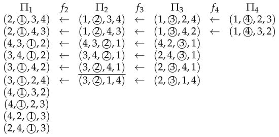
Figure 1. Injective maps $f_2,f_3,f_4$ induced by $G=[50;40,30,20,10]$. The circled number (player) denotes the pivot player.

When an ordered pair of permutations $(\pi ,{\pi }^{\prime })$ satisfies that either (1) $\pi ={\pi }^{\prime }$ or (2) $\pi \in {\Pi }_i$, ${\pi }^{\prime }\in {\Pi }_j$, $i<j$, and $\pi =f_{i-1}\circ \cdots \circ f_{j-1}\circ f_j\left({\pi }^{\prime }\right)$, we say that ${\pi }^{\prime }$ is an ancestor of $\pi$. Here, we note that $\pi$ is always an ancestor of $\pi$ itself. Lemma 1 implies that every permutation $\pi \in {\Pi }_N$ has a unique ancestor, called the originator, ${\pi }^{\prime }\in {\Pi }_j$ satisfying either that $j=n$ or that its inverse image $f_{j+1}^{-1}\left({\pi }^{\prime }\right)=\varnothing$. For each permutation $\pi \in {\Pi }_N$, $\mathrm{org}\left(\pi \right)\in N$ denotes the pivot of the originator of $\pi$; i.e., ${\Pi }_{\mathrm{org}\left(\pi \right)}$ includes the originator of $\pi$.

Now, we describe our algorithm.

Algorithm 2 Our Algorithm.

Step 0: Set $m:=1$, ${\phi }_i^{\prime }:=0(\forall i\in N)$.     Step 1: Choose $\pi \in {\Pi }_N$ uniformly at random. Put the random variable $L^{\left(m\right)}:=\mathrm{org}\left(\pi \right)$.                  Update ${\phi }_i^{\prime }:=\left\{\begin{array}{cc}{\phi }_i^{\prime }+1/L^{\left(m\right)}\hfill & (\mathrm{if}i\le L^{\left(m\right)}),\hfill \\ {\phi }_i^{\prime }\hfill & (\mathrm{if}{L}^{\left(m\right)}<i).\hfill \end{array}\right.$     Step 2: If $m=M$, then output ${\phi }_i^{\prime }/M(\forall i\in N)$ and stop.                  Else, update $m:=m+1$ and go to Step 1.

In the example shown in Figure 1, if we choose $\pi =(3,➁,4,1)$ at Step 1 of Algorithm 2, then $\mathrm{org}\left(\pi \right)=3$, and Algorithm 2 updates

$$({\phi }_1^{\prime },{\phi }_2^{\prime },{\phi }_3^{\prime },{\phi }_4^{\prime }):=({\phi }_1^{\prime }+(1/3),{\phi }_2^{\prime }+(1/3),{\phi }_3^{\prime }+(1/3),{\phi }_4^{\prime }).$$

For each permutation $\pi \in {\Pi }_N$, we can find the originator $\mathrm{org}\left(\pi \right)\in N$ in $\mathrm{O}\left(n\right)$ time. Thus, the time complexity of Algorithm 2 is also bounded by $\mathrm{O}\left(M\right(\tau \left(n\right)+n\left)\right)$, where $\tau \left(n\right)$ denotes the computational effort required for the random generation of a permutation.

We denote the vector (of random variables) obtained by executing Algorithm 2 by $({\phi }_1^{\mathrm{A}2},{\phi }_2^{\mathrm{A}2},\dots ,{\phi }_n^{\mathrm{A}2})$. We have the following properties.

Theorem 3. 

(1) For each player $i\in N$, $\mathrm{E}\left[{\phi }_i^{\mathrm{A}2}\right]={\phi }_i$.

(2) For each pair of players $\{i,j\}\subseteq N$, if ${\phi }_i>{\phi }_j$, then ${\phi }_i^{\mathrm{A}2}\ge {\phi }_j^{\mathrm{A}2}.$

(3) For each pair of players $\{i,j\}\subseteq N$, if ${\phi }_i={\phi }_j$, then ${\phi }_i^{\mathrm{A}2}={\phi }_j^{\mathrm{A}2}.$

Proof. 

(1) For each $i\in N,$ we define that ${\xi }_i=\left|\{\pi \in {\Pi }_N\mid \mathrm{org}\left(\pi \right)=i\}\right|.$ It is obvious that $|{\Pi }_i|={\xi }_i+{\xi }_{i+1}+\cdots +{\xi }_n$$(\forall i\in N).$ If we choose $\pi \in {\Pi }_N$ uniformly at random, then $\mathrm{Pr}[\mathrm{org}\left(\pi \right)=i]=(i·{\xi }_i)/n!$ holds. From the above, it is easy to see that, for each $i\in N$, a random variable $\Delta {\phi }_i^{\prime }\left(\pi \right)$ defined by

$$\Delta {\phi }_i^{\prime }\left(\pi \right):=\left\{\begin{array}{cc}1/\mathrm{org}\left(\pi \right)\hfill & (\mathrm{if}i\le \mathrm{org}(\pi \left)\right),\hfill \\ 0\hfill & \left(\mathrm{if}\mathrm{org}\right(\pi )<i),\hfill \end{array}\right.$$

satisfies that

$$\begin{array}{cc}\hfill \mathrm{E}[& \Delta {\phi }_i^{\prime }\left(\pi \right)]\hfill \\ & = \mathrm{Pr}[\mathrm{org}\left(\pi \right)=i]\left(\frac{1}{i}\right)+\mathrm{Pr}[\mathrm{org}\left(\pi \right)=i+1]\left(\frac{1}{i+1}\right)+\cdots +\mathrm{Pr}[\mathrm{org}\left(\pi \right)=n]\left(\frac{1}{n}\right)\hfill \\ & = \left(\frac{i·{\xi }_i}{n!}\right)\left(\frac{1}{i}\right)+\left(\frac{(i+1)·{\xi }_{i+1}}{n!}\right)\left(\frac{1}{i+1}\right)+\cdots +\left(\frac{n·{\xi }_n}{n!}\right)\left(\frac{1}{n}\right)\hfill \\ & = \frac{{\xi }_i+{\xi }_{i+1}+\cdots +{\xi }_n}{n!}=\frac{|{\Pi }_i|}{n!}={\phi }_i.\hfill \end{array}$$

When $({\pi }^{\left(1\right)},{\pi }^{\left(2\right)},\dots ,{\pi }^{\left(M\right)})$ denotes a sequence of permutations generated in Algorithm 2, we have that

$$\begin{array}{ccc}\hfill \mathrm{E}\left[{\phi }_i^{\mathrm{A}2}\right]& =& \mathrm{E}\left[\frac{\Delta {\phi }_i^{\prime }\left({\pi }^{\left(1\right)}\right)+\Delta {\phi }_i^{\prime }\left({\pi }^{\left(2\right)}\right)+\cdots +\Delta {\phi }_i^{\prime }\left({\pi }^{\left(M\right)}\right)}{M}\right]=\sum _{m=1}^M\frac{\mathrm{E}[\Delta {\phi }_i^{\prime }\left({\pi }^{\left(m\right)}\right)]}{M}\hfill \\ & =& \sum _{m=1}^M\frac{{\phi }_i}{M}={\phi }_i.\hfill \end{array}$$

(2) Assumption 1 implies that, if ${\phi }_i>{\phi }_j$, then $w_i>w_j$, and thus, $i<j$. The update formula of ${\phi }_i^{\prime }$ in Algorithm 2 directly implies that inequalities ${\phi }_1^{\prime }\ge {\phi }_2^{\prime }\ge \cdots \ge {\phi }_n^{\prime }$ hold throughout the iterations of Algorithm 2, which leads to inequalities ${\phi }_1^{\mathrm{A}2}\ge {\phi }_2^{\mathrm{A}2}\ge \cdots \ge {\phi }_n^{\mathrm{A}2}$. From the above, we obtain that ${\phi }_i^{\mathrm{A}2}\ge {\phi }_j^{\mathrm{A}2}.$

(3) In the following, we assume that ${\phi }_i={\phi }_j$ and $i<j$. Assumption 1 implies that ${\phi }_i={\phi }_{i+1}=\cdots ={\phi }_j$, and thus, $|{\Pi }_i|=|{\Pi }_{i+1}|=\cdots =|{\Pi }_j|.$ From Lemma 1, $f_{i+1},\dots ,f_j$ are bijections; thus, $\forall \pi \in \Pi ,\mathrm{org}\left(\pi \right)\notin \{i,i+1,\dots ,j-1\}.$ Then, the update formula of ${\phi }_i^{\prime }$ in Algorithm 2 implies that equalities ${\phi }_i^{\prime }={\phi }_{i+1}^{\prime }=\cdots ={\phi }_j^{\prime }$ hold throughout the iterations of Algorithm 2, which leads to the desired result: ${\phi }_i^{\mathrm{A}2}={\phi }_{i+1}^{\mathrm{A}2}=\cdots ={\phi }_j^{\mathrm{A}2}$. □

The following theorem provides the number of samples required in Algorithm 2.

Theorem 4.

For any $\epsilon >0$ and $0<\delta <1$, we have the following.

(1) For each player $i\in N=\{1,2,\dots ,n\}$, if we set ${\displaystyle M\ge \frac{ln2+ln(1/\delta )}{2{\epsilon }^2{i}^2}}$, then

$$\mathrm{Pr}\left[\left|{\phi }_i^{\mathrm{A}2}-{\phi }_i\right|<\epsilon \right]\ge 1-\delta .$$

(2) If we set ${\displaystyle M\ge \frac{ln2+ln(1/\delta )}{2{\epsilon }^2}}$, then

$$\begin{array}{ccc}\hfill \mathrm{Pr}\left[\forall i\in N,\left|{\phi }_i^{\mathrm{A}2}-{\phi }_i\right|<\epsilon \right]& \ge & 1-2\sum _{i=1}^n{\left(\frac{\delta }{2}\right)}^{i^2}\hfill \\ & =& 1-2\left(\left(\frac{\delta }{2}\right)+{\left(\frac{\delta }{2}\right)}^4+{\left(\frac{\delta }{2}\right)}^9+\cdots +{\left(\frac{\delta }{2}\right)}^{n^2}\right).\hfill \end{array}$$

(3) If we set ${\displaystyle M\ge \frac{|N^{*}|ln2+ln(1/\delta )}{2{\epsilon }^2}}$, then

$$\mathrm{Pr}\left[\frac{1}{2}\sum _{i\in N}\left|{\phi }_i^{\mathrm{A}2}-{\phi }_i\right|<\epsilon \right]\ge 1-\delta ,$$

where $N^{*}=\{i\in N\backslash \left\{n\right\}\mid {\phi }_i>{\phi }_{i+1}\}\cup \left\{n\right\}$, i.e., $|N^{*}|$ is equal to the size of the maximal player subset, the S–S indices of which are mutually different.

Proof. 

Let us introduce random variables $X_i^{\left(m\right)}(\forall m\in \{1,2,\dots ,M\},\forall i\in N)$ in Step 2 of Algorithm 2, defined by

$$X_i^{\left(m\right)}=\left\{\begin{array}{cc}1/L^{\left(m\right)}\hfill & (\mathrm{if}1\le i\le L^{\left(m\right)}),\hfill \\ 0\hfill & (\mathrm{if}{L}^{\left(m\right)}<i).\hfill \end{array}\right.$$

It is obvious that, for each player $i\in N$, $\{X_i^{\left(1\right)},X_i^{\left(2\right)},\dots ,X_i^{\left(M\right)}\}$ is a collection of independent and identically distributed random variables satisfying

$${\phi }_i^{\mathrm{A}2}=\sum _{m=1}^M{X}_i^{\left(m\right)}/M,\mathrm{E}\left[{\phi }_i^{\mathrm{A}2}\right]=\mathrm{E}\left[X_i^{\left(m\right)}\right]={\phi }_i,\mathrm{and}(1/i)\ge X_i^{\left(m\right)}\ge (1/n)$$

for all $m\in \{1,2,\dots ,M\}.$ Hoeffding’s inequality [40] implies that each player $i\in N$ satisfies

$$\begin{array}{ccc}\hfill \mathrm{Pr}\left[\left|{\phi }_i^{\mathrm{A}2}-{\phi }_i\right|\ge \epsilon \right]& \le & 2exp\left(-\frac{2M^2{\epsilon }^2}{{\sum }_{m=1}^M{(1/i-0)}^2}\right)=2exp(-2M{\epsilon }^2{i}^2).\hfill \end{array}$$

(1) If we set ${\displaystyle M\ge \frac{ln(2/\delta )}{2{\epsilon }^2{i}^2}}$, then

$$\mathrm{Pr}\left[\left|{\phi }_i^{\mathrm{A}2}-{\phi }_i\right|<\epsilon \right]\ge 1-2exp\left(-2\frac{ln(2/\delta )}{2{\epsilon }^2{i}^2}{\epsilon }^2{i}^2\right)=1-\delta .$$

(2) If we set ${\displaystyle M\ge \frac{ln(2/\delta )}{2{\epsilon }^2}}$, then we have that

$$\begin{gathered} {\displaystyle \mathrm{Pr}\left[\forall i\in N,\left|{\phi }_i^{\mathrm{A}2}-{\phi }_i\right|<\epsilon \right]=1-\mathrm{Pr}\left[\exists i\in N,\left|{\phi }_i^{\mathrm{A}2}-{\phi }_i\right|\ge \epsilon \right]} \\ \ge 1-\sum _{i\in N}\mathrm{Pr}\left[\left|{\phi }_i^{\mathrm{A}2}-{\phi }_i\right|\ge \epsilon \right]\ge 1-\sum _{i=1}^{n}2exp(-2M{\epsilon }^2{i}^2) \\ \ge 1-2\sum _{i=1}^{n}exp\left(-2\frac{ln(2/\delta )}{2{\epsilon }^2}{\epsilon }^2{i}^2\right)=1-2\sum _{i=1}^n{\left(\frac{\delta }{2}\right)}^{i^2}. \end{gathered}$$

(3) We introduce random variables $Y_{\ell }^{\left(m\right)}$ $(\forall m\in \{1,2,\dots ,M\},\forall \ell \in N)$ in Step 2 of Algorithm 2, defined by

$$Y_{\ell }^{\left(m\right)}=\left\{\begin{array}{cc}1\hfill & (\mathrm{if}\ell =L^{\left(m\right)}),\hfill \\ 0\hfill & \left(\mathrm{otherwise}\right).\hfill \end{array}\right.$$

Because ${\sum }_{\ell =1}^n{Y}_{\ell }^{\left(m\right)}=1$$(\forall m)$, the above definition directly implies that

$$X_i^{\left(m\right)}=\frac{1}{i}{Y}_i^{\left(m\right)}+\frac{1}{i+1}{Y}_{i+1}^{\left(m\right)}+\cdots +\frac{1}{n}{Y}_n^{\left(m\right)}.$$

For each player $i\in N$ and $i\le \forall \ell \le n$, we define ${\Pi }_{i\ell }=\{\pi \in {\Pi }_i\mid \mathrm{org}\left(\pi \right)=\ell \}$. It is easy to show that $|{\Pi }_{1\ell }|=|{\Pi }_{2\ell }|=\cdots =|{\Pi }_{\ell \ell }|$ for each $\ell \in \{1,2,\dots ,n\}$. The above definitions imply that

$$\begin{array}{cc}\hfill \frac{1}{2}& \sum _{i\in N}\left|{\phi }_i^{\mathrm{A}2}-{\phi }_i\right|=\frac{1}{2M}\sum _{i\in N}\left|M{\phi }_i^{\mathrm{A}2}-M{\phi }_i\right|=\frac{1}{2M}\sum _{i\in N}\left|\sum _{m=1}^M{X}_i^{\left(m\right)}-M\frac{|{\Pi }_i|}{n!}\right|\hfill \\ & = \frac{1}{2M}\sum _{i\in N}\left|\sum _{m=1}^M\sum _{\ell =i}^n\frac{1}{\ell }{Y}_{\ell }^{\left(m\right)}-\frac{M}{n!}\sum _{\ell =i}^n\left|{\Pi }_{i\ell }\right|\right|\hfill \\ & = \frac{1}{2M}\sum _{i\in N}\left|\sum _{\ell =i}^n\left(\sum _{m=1}^M\frac{1}{\ell }{Y}_{\ell }^{\left(m\right)}-\frac{M}{n!}\left|{\Pi }_{i\ell }\right|\right)\right|\hfill \\ & \le \frac{1}{2M}\sum _{i=1}^n\sum _{\ell =i}^n\left|\sum _{m=1}^M\frac{1}{\ell }{Y}_{\ell }^{\left(m\right)}-\frac{M}{n!}\left|{\Pi }_{i\ell }\right|\right|=\frac{1}{2M}\sum _{\ell =1}^n\sum _{i=1}^{\ell }\left|\sum _{m=1}^M\frac{1}{\ell }{Y}_{\ell }^{\left(m\right)}-\frac{M}{n!}\left|{\Pi }_{i\ell }\right|\right|\hfill \\ & = \frac{1}{2M}\sum _{\ell =1}^n\ell \left|\sum _{m=1}^M\frac{1}{\ell }{Y}_{\ell }^{\left(m\right)}-\frac{M}{n!}\left|{\Pi }_{1\ell }\right|\right|\left(\mathrm{since}\right|{\Pi }_{1\ell }|=|{\Pi }_{2\ell }|=\cdots =|{\Pi }_{\ell \ell }\left|\right)\hfill \\ & = \frac{1}{2M}\sum _{\ell =1}^n\left|\sum _{m=1}^M{Y}_{\ell }^{\left(m\right)}-\frac{M\ell }{n!}\left|{\Pi }_{1\ell }\right|\right|.\hfill \end{array}$$

For each player $\ell \notin N^{*}$, we have the equalities $|{\Pi }_{\ell }|=n!{\phi }_{\ell }=n!{\phi }_{\ell +1}=\left|{\Pi }_{\ell +1}\right|$, which yields that $f_{\ell +1}:{\Pi }_{\ell +1}\to {\Pi }_{\ell }$ is a bijection; thus, ${\Pi }_{\ell }$ does not include any originator. From the above, it is obvious that, if $\ell \notin N^{*}$, then ${\Pi }_{1\ell }={\Pi }_{2\ell }=\cdots ={\Pi }_{\ell \ell }=\varnothing$. For each $\ell \in \{1,2,\dots ,n\}$, $\{Y_{\ell }^{\left(1\right)},Y_{\ell }^{\left(2\right)},\dots ,Y_{\ell }^{\left(M\right)}\}$ is a Bernoulli process satisfying $\mathrm{E}\left[Y_{\ell }^{\left(m\right)}\right]=\frac{1}{n!}{\sum }_{i=1}^{\ell }|{\Pi }_{i\ell }|=\frac{\ell }{n!}\left|{\Pi }_{1\ell }\right|$$(\forall m)$. Thus, $\ell \notin N^{*}$ implies that $Y_{\ell }^{\left(m\right)}=0$ for any $m\in \{1,2,\dots ,M\}$. To summarize the above, we have shown that

$$\mathrm{if}\ell \notin N^{*}\mathrm{then}\sum _{m=1}^M{Y}_{\ell }^{\left(m\right)}-\frac{M\ell }{n!}\left|{\Pi }_{1\ell }\right|=\sum _{m=1}^{M}0-\frac{M\ell }{n!}0=0.$$

Now, we have an upper bound of the total variation distance

$$\begin{array}{ccc}\hfill \frac{1}{2}\sum _{i\in N}\left|{\phi }_i^{\mathrm{A}2}-{\phi }_i\right|& \le & \frac{1}{2M}\sum _{\ell =1}^n\left|\sum _{m=1}^M{Y}_{\ell }^{\left(m\right)}-\frac{M\ell }{n!}\left|{\Pi }_{1\ell }\right|\right|\hfill \\ & =& \frac{1}{2M}\sum _{\ell \in N^{*}}\left|\sum _{m=1}^M{Y}_{\ell }^{\left(m\right)}-\sum _{m=1}^M\mathrm{E}\left[Y_{\ell }^{\left(m\right)}\right]\right|.\hfill \end{array}$$

The vector of random variables ${\left({\sum }_{m=1}^M{Y}_{\ell }^{\left(m\right)}\right)}_{\ell \in N^{*}}$ is multinomially distributed and satisfies that the total sum is equal to M. Then, the Bretagnolle–Huber–Carol inequality [41] (Theorem A1 in Appendix A) implies that

$$\begin{array}{cc}\hfill \mathrm{Pr}& \left[\frac{1}{2}\sum _{i\in N}\left|{\phi }_i^{\mathrm{A}2}-{\phi }_i\right|\ge \epsilon \right]\le \mathrm{Pr}\left[\frac{1}{2M}\sum _{\ell \in N^{*}}\left|\sum _{m=1}^M{Y}_{\ell }^{\left(m\right)}-\sum _{m=1}^M\mathrm{E}\left[Y_{\ell }^{\left(m\right)}\right]\right|\ge \epsilon \right]\hfill \\ & = \mathrm{Pr}\left[\sum _{\ell \in N^{*}}\left|\sum _{m=1}^M{Y}_{\ell }^{\left(m\right)}-\sum _{m=1}^M\mathrm{E}\left[Y_{\ell }^{\left(m\right)}\right]\right|\ge 2M\epsilon \right]\le 2^{|N^{*}|}exp\left(-2M{\epsilon }^2\right)\hfill \\ & \le 2^{|N^{*}|}exp\left(-2\frac{ln\left(2^{|N^{*}|}/\delta \right)}{2{\epsilon }^2}{\epsilon }^2\right)=\delta \hfill \end{array}$$

and thus, we have the desired result. □

The following corollary provides an approximate version of Theorem 4 (2). Surprisingly, it says that the required number of samples is irrelevant to n (number of players).

Corollary 1.

For any $\epsilon >0$ and $0<{\delta }^{\prime }<1$, we have the following.

If we set ${\displaystyle M\ge \frac{ln2+ln(1/{\delta }^{\prime })+ln1.129}{2{\epsilon }^2}}$, then

$$\mathrm{Pr}\left[\forall i\in N,\left|{\phi }_i^{\mathrm{A}2}-{\phi }_i\right|<\epsilon \right]\ge 1-{\delta }^{\prime }.$$

Proof. 

If we put $\delta ={\delta }^{\prime }/1.129$, then Theorem 2 (2) implies that

$$\begin{array}{cc}\hfill \mathrm{Pr}& \left[\forall i\in N,\left|{\phi }_i^{A2}-{\phi }_i\right|<\epsilon \right]\hfill \\ & \ge 1-2\left(\left(\frac{\delta }{2}\right)+{\left(\frac{\delta }{2}\right)}^4+{\left(\frac{\delta }{2}\right)}^9+\cdots +{\left(\frac{\delta }{2}\right)}^{n^2}\right)\hfill \\ & \ge 1-\delta \left(1+{\left(\frac{1}{2}\right)}^3+{\left(\frac{1}{2}\right)}^8+{\left(\frac{1}{2}\right)}^{15}+{\left(\frac{1}{2}\right)}^{24}+\cdots +{\left(\frac{1}{2}\right)}^{n^2-1}\right)\hfill \\ & \ge 1-\delta \left(1+{\left(\frac{1}{2}\right)}^3+{\left(\frac{1}{2}\right)}^8\left(1+{\left(\frac{1}{2}\right)}^7+{\left(\frac{1}{2}\right)}^{14}+{\left(\frac{1}{2}\right)}^{21}+\cdots \right)\right)\hfill \\ & = 1-\delta \left(1+{\left(\frac{1}{2}\right)}^3+{\left(\frac{1}{2}\right)}^8\left(\frac{1}{1-{(1/2)}^7}\right)\right)\ge 1-1.129\delta =1-{\delta }^{\prime }.\hfill \end{array}$$

□

Here, we note that $ln2\simeq 0.69314$ and $ln1.129\simeq 0.12133$.

In a practical setting, it is difficult to estimate the size of $N^{*}$ defined in Theorem 4 (3) since the problem of verifying the asymmetricity of a given pair of players is NP-complete [19]. The following corollary is useful in some practical situations.

Corollary 2.

For any $\epsilon >0$ and $0<\delta <1$, we have the following.

If we set ${\displaystyle M\ge \frac{n^{″}ln2+ln(1/\delta )}{2{\epsilon }^2}}$, then

$$\mathrm{Pr}\left[\frac{1}{2}\sum _{i\in N}\left|{\phi }_i^{\mathrm{A}2}-{\phi }_i\right|<\epsilon \right]\ge 1-\delta ,$$

where $n^{″}=|\{i\in N\backslash \left\{n\right\}\mid w_i>w_{i+1}\}\cup \left\{n\right\}|$, i.e., $n^{″}$ is equal to the size of a maximal player subset with mutually different weights.

Proof. 

Since ${\phi }_i>{\phi }_{i+1}$ implies $w_i>w_{i+1}$, it is obvious that $|N^{*}|\le n^{″}$, and we have the desired result. □

A game of the power of the countries in the EU Council is defined by (255; 29, 29, 29, 29, 27, 27, 14, 13, 12, 12, 12, 12, 12, 10, 10, 10, 7, 7, 7, 7, 7, 4, 4, 4, 4, 4, 3) [42,43]. In this case, $n=27$ and $n^{″}=9$. A weighted majority game defined by [44] (Section 12.4) for a voting process in the United States has a vector of weights

$$\begin{array}{c}(270;45,41,27,26,26,25,21,17,17,14,13,13,12,12,12,11,\underset{4\mathrm{times}}{\underbrace{10,\dots ,10}},\underset{4\mathrm{times}}{\underbrace{9,\dots ,9}},\hfill \\ 8,8,\underset{4\mathrm{times}}{\underbrace{7,\dots ,7}},\underset{4\mathrm{times}}{\underbrace{6,\dots ,6}},5,\underset{9\mathrm{times}}{\underbrace{4,\dots ,4}},\underset{7\mathrm{times}}{\underbrace{3,\dots ,3}}),\mathrm{where}n=51\mathrm{and}{n}^{″}=19.\hfill \end{array}$$

5. Computational Experiments

This section reports the results of our preliminary numerical experiments. All the experiments were conducted on a Windows machine, i7-7700 CPU@3.6GHz Memory (RAM) 16 GB. Algorithms 1 and 2 were implemented using Python 3.6.5.

We tested the EU Council instance and the United States instance described in the previous section. In each instance, we set M in Algorithms 1 and 2 (the number of generated permutations) to $M\in \{1\times {10}^5,2\times {10}^5,\dots ,24\times {10}^5\}$. For each value of M, we executed Algorithms 1 and 2 100 times. Figure 2 and Figure 3 show the results of some players. For each value of M, we calculated the mean number of $|{\phi }_i-{\phi }_i^{\mathrm{A}}|$, denoted by $\widehat{{\epsilon }_i}$, in an average of 100 trials. The horizontal axes of Figure 2 and Figure 3 show the value $1/{\widehat{{\epsilon }_i}}^2$. Under the assumption that $M=\alpha /{\widehat{{\epsilon }_i}}^2$, we estimated $\alpha$ by the least squares method. Table 2 shows the results and ratios of $\alpha$ of the two algorithms.

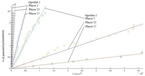
Figure 2. EU Council.

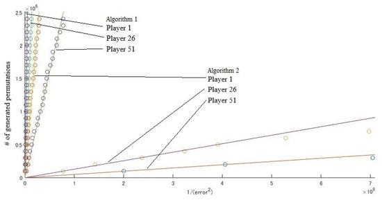
Figure 3. United States.

Table 2. Comparison of Algorithms 1 and 2.

EU Council	$\mathit{\alpha }$
	Algorithm 1	Algorithm 2	ratio
Player 1	0.0557	0.0022	25.318
Player 13	0.0199	$4.1615\times {10}^{-4}$	47.819
Player 27	0.0049	$1.3987\times {10}^{-4}$	35.033
United States	$\alpha$
	Algorithm 1	Algorithm 2	ratio
Player 1	0.0489	0.0181	2.7017
Player 26	0.0088	$1.2837\times {10}^{-4}$	68.552
Player 51	0.0032	$4.8911\times {10}^{-5}$	65.424

For each (generated) permutation, the computational effort of both Algorithms 1 and 2 are bounded by $\mathrm{O}\left(n\right)$. Here, we discuss the constant factors of $\mathrm{O}\left(n\right)$ computations. We tested the cases where weights $w_i$ are generated uniformly at random from the intervals $(1,10)$ or $(1,20)$, and the quota is equal to $(1/2){\sum }_{i\in N}{w}_i$. For each $n\in \{10,20,\dots ,100\}$, we executed Algorithms 1 and 2 by setting M = 10,000. Under the assumption that computational time is equal to $an+b$, we estimated a and b by the least squares method. Figure 4 shows that for each permutation, the computational effort of Algorithm 2 increases about five-fold compared to Algorithm 1.

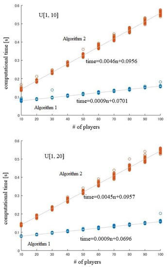
Figure 4. Computational time.

6. Conclusions

In this paper, we analyzed a naive Monte Carlo algorithm (Algorithm 1) for calculating the S–S index denoted by $({\phi }_1,{\phi }_2,\dots ,{\phi }_n)$ in weighted majority games. By employing the Bretagnolle–Huber–Carol inequality [41] (Theorem A1 in Appendix A), we estimated the required number of samples that gives an upper bound of the total variation distance.

We also proposed an efficient Monte Carlo algorithm (Algorithm 2). The time complexity of each iteration of our algorithm is equal to that of the naive algorithm (Algorithm 1). Our algorithm has the property that the obtained estimator $({\phi }_1^{\mathrm{A}2},{\phi }_2^{\mathrm{A}2},\dots ,{\phi }_n^{\mathrm{A}2})$ satisfies

$$\mathrm{both}[\mathrm{if}{\phi }_i<{\phi }_j,\mathrm{then}{\phi }_i^{\mathrm{A}2}\le {\phi }_j^{\mathrm{A}2}]\mathrm{and}[\mathrm{if}{\phi }_i={\phi }_j,\mathrm{then}{\phi }_i^{\mathrm{A}2}={\phi }_j^{\mathrm{A}2}].$$

We proved that, even if we consider the property

$$\mathrm{Pr}\left[\forall i\in N,\left|{\phi }_i^{\mathrm{A}2}-{\phi }_i\right|<\epsilon \right]\ge 1-\delta ,$$

the required number of samples is irrelevant to n (the number of players).

References

- Von Neumann, J.; Morgenstern, O. Theory of Games and Economic Behavior; Princeton University Press: Princeton, NJ, USA, 1944. [Google Scholar]
- Shapley, L.S.; Shubik, M. A method for evaluating the distribution of power in a committee system. Am. Political Sci. Rev. 1954, 48, 787–792. [Google Scholar] [CrossRef]
- Shapley, L.S. A value for n-person games. In Contributions to the Theory of Games II; Kuhn, H.W., Tucker, A.W., Eds.; Princeton University Press: Princeton, NJ, USA, 1953; pp. 307–317. [Google Scholar]
- Laruelle, A.; Widgrén, M. Is the allocation of voting power among EU states fair? Public Choice 1998, 94, 317–339. [Google Scholar] [CrossRef]
- Leech, D. Designing the voting system for the Council of the European Union. Public Choice 2002, 113, 437–464. [Google Scholar] [CrossRef]
- Życzkowski, K.; Słomczyński, W. Square Root Voting System, Optimal Threshold and π. In Power, Voting, and Voting Power: 30 Years After; Springer: Berlin/Heidelberg, Germany, 2013; pp. 573–592. [Google Scholar]
- Owen, G. Evaluation of a presidential election game. Am. Political Sci. Rev. 1975, 69, 947–953. [Google Scholar] [CrossRef]
- Miller, N.R. A priori voting power and the US Electoral College. In Power, Voting, and Voting Power: 30 Years After; Springer: Berlin/Heidelberg, Germany, 2013; pp. 411–442. [Google Scholar]
- Leech, D. Voting power in the governance of the International Monetary Fund. Ann. Oper. Res. 2002, 109, 375–397. [Google Scholar] [CrossRef]
- Leech, D.; Leech, R. A new analysis of a priori voting power in the IMF: Recent quota reforms give little cause for celebration. In Power, Voting, and Voting Power: 30 Years After; Springer: Berlin/Heidelberg, Germany, 2013; pp. 389–410. [Google Scholar]
- Young, H.P. Cost allocation. Handb. Game Theory Econ. Appl. 1994, 2, 1193–1235. [Google Scholar]
- Lucchetti, R.; Radrizzani, P. Microarray data analysis via weighted indices and weighted majority games. In International Meeting on Computational Intelligence Methods for Bioinformatics and Biostatistics; Springer: Berlin/Heidelberg, Germany, 2009; pp. 179–190. [Google Scholar]
- Holler, M.J.; Rupp, F. Power in networks: A PGI analysis of Krackhardt’s Kite Network. In Transactions on Computational Collective Intelligence XXXIV; Springer: Berlin/Heidelberg, Germany, 2019; pp. 21–34. [Google Scholar]
- Holler, M.J.; Rupp, F. Power in Networks: The Medici. Homo Oeconomicus 2021, 38, 59–75. [Google Scholar] [CrossRef]
- Bachrach, Y.; Rosenschein, J.S.; Porat, E. Power and stability in connectivity games. In Proceedings of the 7th International Joint Conference on Autonomous Agents and Multiagent Systems, Estoril, Portugal, 12–16 May 2008; Volume 2, pp. 999–1006. [Google Scholar]
- Garey, M.R.; Johnson, D.S. Computers and Intractability; Freeman: San Francisco, CA, USA, 1979; Volume 174. [Google Scholar]
- Deng, X.; Papadimitriou, C.H. On the complexity of cooperative solution concepts. Math. Oper. Res. 1994, 19, 257–266. [Google Scholar] [CrossRef]
- Prasad, K.; Kelly, J.S. NP-completeness of some problems concerning voting games. Int. J. Game Theory 1990, 19, 1–9. [Google Scholar] [CrossRef]
- Matsui, Y.; Matsui, T. NP-completeness for calculating power indices of weighted majority games. Theor. Comput. Sci. 2001, 263, 305–310. [Google Scholar] [CrossRef]
- Elkind, E.; Goldberg, L.A.; Goldberg, P.W.; Wooldridge, M. Computational complexity of weighted threshold games. In AAAI; Association for the Advancement of Artificial Intelligence: Menlo Park, CA, USA, 2007; pp. 718–723. [Google Scholar]
- Mann, I.; Shapley, L.S. Values of Large Games, IV: Evaluating the Electoral College by Montecarlo Techniques; Technical Report RM-2651; The RAND Corporation: Santa Monica, CA, USA, 1960. [Google Scholar]
- Matsui, T.; Matsui, Y. A survey of algorithms for calculating power indices of weighted majority games. J. Oper. Res. Soc. Jpn. 2000, 43, 71–86. [Google Scholar] [CrossRef][Green Version]
- Fatima, S.S.; Wooldridge, M.; Jennings, N.R. A linear approximation method for the Shapley value. Artif. Intell. 2008, 172, 1673–1699. [Google Scholar] [CrossRef]
- Castro, J.; Gómez, D.; Tejada, J. Polynomial calculation of the Shapley value based on sampling. Comput. Oper. Res. 2009, 36, 1726–1730. [Google Scholar] [CrossRef]
- Bachrach, Y.; Markakis, E.; Resnick, E.; Procaccia, A.D.; Rosenschein, J.S.; Saberi, A. Approximating power indices: Theoretical and empirical analysis. Auton. Agents-Multi-Agent Syst. 2010, 20, 105–122. [Google Scholar] [CrossRef]
- Castro, J.; Gómez, D.; Molina, E.; Tejada, J. Improving polynomial estimation of the Shapley value by stratified random sampling with optimum allocation. Comput. Oper. Res. 2017, 82, 180–188. [Google Scholar] [CrossRef]
- Owen, G. Multilinear extensions of games. Manag. Sci. 1972, 18, 64–79. [Google Scholar] [CrossRef]
- Leech, D. Computing power indices for large voting games. Manag. Sci. 2003, 49, 831–837. [Google Scholar] [CrossRef]
- Brams, S.J.; Affuso, P.J. Power and size: A new paradox. Theory Decis. 1976, 7, 29–56. [Google Scholar] [CrossRef]
- Lucas, W.F. Measuring power in weighted voting systems. In Political and Related Models; Springer: Berlin/Heidelberg, Germany, 1983; pp. 183–238. [Google Scholar]
- Mann, I.; Shapley, L.S. Values of Large Games, VI: Evaluating the Electoral College Exactly; Technical Report RM-3158-PR; The RAND Corporation: Santa Monica, CA, USA, 1962. [Google Scholar]
- Uno, T. Efficient computation of power indices for weighted majority games. In International Symposium on Algorithms and Computation; Springer: Berlin/Heidelberg, Germany, 2012; pp. 679–689. [Google Scholar]
- Bilbao, J.M.; Fernandez, J.R.; Jiménez-Losada, A.; Lopez, J.J. Generating functions for computing power indices efficiently. Top 2000, 8, 191–213. [Google Scholar] [CrossRef]
- Bolus, S. Power indices of simple games and vector-weighted majority games by means of binary decision diagrams. Eur. J. Oper. Res. 2011, 210, 258–272. [Google Scholar] [CrossRef]
- Rushdi, A.M.A.; Ba-Rukab, O.M. Map calculation of the Shapley-Shubik voting powers: An example of the European Economic Community. Int. J. Math. Eng. Manag. Sci. 2017, 2, 17–29. [Google Scholar] [CrossRef]
- Berghammer, R.; Bolus, S.; Rusinowska, A.; De Swart, H. A relation-algebraic approach to simple games. Eur. J. Oper. Res. 2011, 210, 68–80. [Google Scholar] [CrossRef]
- Klinz, B.; Woeginger, G.J. Faster algorithms for computing power indices in weighted voting games. Math. Soc. Sci. 2005, 49, 111–116. [Google Scholar] [CrossRef]
- Alonso-Meijide, J.M.; Casas-Méndez, B.; Fiestras-Janeiro, M.G. Computing Banzhaf–Coleman and Shapley–Shubik power indices with incompatible players. Appl. Math. Comput. 2015, 252, 377–387. [Google Scholar] [CrossRef]
- Courtin, S.; Nganmeni, Z.; Tchantcho, B. The Shapley–Shubik power index for dichotomous multi-type games. Theory Decis. 2016, 81, 413–426. [Google Scholar] [CrossRef]
- Hoeffding, W. Probability inequalities for sums of bounded random variables. J. Am. Stat. Assoc. 1963, 58, 13–30. [Google Scholar] [CrossRef]
- van der Vaart, A.W.; Wellner, J.A. Weak Convergence and Empirical Processes: With Applications to Statistics; Springer Science & Business Media: Berlin/Heidelberg, Germany, 1996. [Google Scholar]
- Felsenthal, D.S.; Machover, M. The Treaty of Nice and qualified majority voting. Soc. Choice Welf. 2001, 18, 431–464. [Google Scholar] [CrossRef]
- Bilbao, J.M.; Fernandez, J.R.; Jiménez, N.; Lopez, J.J. Voting power in the European Union enlargement. Eur. J. Oper. Res. 2002, 143, 181–196. [Google Scholar] [CrossRef][Green Version]
- Owen, G. Game Theory; Academic Press: Cambridge, MA, USA, 1995. [Google Scholar]
Publisher’s Note: MDPI stays neutral with regard to jurisdictional claims in published maps and institutional affiliations. |
© 2022 by the authors. Licensee MDPI, Basel, Switzerland. This article is an open access article distributed under the terms and conditions of the Creative Commons Attribution (CC BY) license (https://creativecommons.org/licenses/by/4.0/).