Partial Order Games

Abstract

We introduce a non-cooperative game model in which players’ decision nodes are partially ordered by a dependence relation, which directly captures informational dependencies in the game. In saying that a decision node v is dependent on decision nodes $v_1,\dots ,v_k$, we mean that the information available to a strategy making a choice at v is precisely the choices that were made at $v_1,\dots ,v_k$. Although partial order games are no more expressive than extensive form games of imperfect information (we show that any partial order game can be reduced to a strategically equivalent extensive form game of imperfect information, though possibly at the cost of an exponential blowup in the size of the game), they provide a more natural and compact representation for many strategic settings of interest. After introducing the game model, we investigate the relationship to extensive form games of imperfect information, the problem of computing Nash equilibria, and conditions that enable backwards induction in this new model.

1. Introduction

The two most important game models in non-cooperative game theory are normal form games and extensive form games. These games are distinguished by the information that players have about the strategies of other players. In normal form games, players must select and commit to strategies without any information relating to the strategies of others. In contrast, in extensive form games, players make moves alternately over time and, during play, their strategy may be informed by moves made previously. Variations of extensive form games—e.g., of imperfect information or recall—make it possible to capture the information available to a player when called upon to make a move.

In this article, we introduce partial order games. The key distinguishing feature of partial order games is that they are equipped with a dependence relation, which explicitly captures the informational dependencies between decision nodes. In saying that a decision node v is dependent on decision nodes $v_1,\dots ,v_k$, we mean that the information available to a strategy making a choice at v is precisely the choices that were made at $v_1,\dots ,v_k$. Observe that the informational dependencies captured by a dependence relation give rise to a partial temporal order over choices: in this case, the choices for $v_1,\dots ,v_k$ must strictly precede the choice for v. However, the temporal ordering induced in this way is indeed partial: it may be that two choices $v^{\prime }$ and $v^{″}$ are independent, in which case one can say nothing about their temporal order.

In a technical sense, partial order games are no more expressive than extensive form games of imperfect information: one of our key results is to show that every partial order game can be transformed into a strategically equivalent extensive form game of imperfect information. However, for some settings, partial order games have significant advantages over their extensive form representation:

• First, informational dependencies in partial order games are explicitly captured, while in extensive form games, they are left implicit in the information sets of the game. As a consequence, some settings are much more transparently and naturally represented using partial order games, compared to the extensive form.
• Second, partial order games can be exponentially more compact than their extensive form. From a purely practical point of view, this means that some scenarios with a compact partial order representation cannot be handled (by people or by a computer) in their extensive form.

We analyse partial order games by means of Nash equilibrium—arguably game theory’s most prominent non-cooperative solution concept—and the solutions given by a natural backwards induction procedure for partial order games defined on the dependence relation. Here, we give special attention to the computational complexity of calculating such solutions in partial order games. The remainder of this article is structured as follows.

• We begin by briefly recalling some necessary concepts from graph theory and game theory, and then introduce the formal framework of partial order games.
• As we are interested in the computational properties of partial order games, we introduce a compact representation for strategies and utility functions in partial order games, based on Boolean circuits, which enables us to investigate questions about their computational complexity.
• In Section 4, we study the relationship of our game model to other game models: partial order Boolean games [1], Multi-Agent Influence Diagrams (MAIDs) [2,3], and extensive form games of imperfect information. Our main result in this section is to present a technique for translating partial order games into strategically equivalent extensive form games, although this translation comes at the cost of an exponential blowup in the size of the game. This leads us into a discussion of the use of partial order games as a compact representation of extensive form games.
• In Section 5, we investigate the problem of computing Nash equilibria in partial order games. For example, we show that checking whether a game has any pure strategy Nash equilibria is NEXPTIME-complete.
• In Section 6, we study backwards induction in partial order games. As partial order games are inherently games of imperfect information, it follows that backwards induction does not always work for partial order games. We thus investigate cases where forms of backward induction work for partial order games, and present a condition on games that we call fit for backwards induction, which is sufficient to allow backwards induction.
• We conclude with a brief discussion and pointers for future work.

2. Preliminary Definitions

We begin by recalling some concepts from graph theory and game theory, which we use in the remainder of the paper.

2.1. Directed Acyclic Graphs and Trees

The games in this paper are defined on directed acyclic graphs (DAGs). Formally, a directed acyclic graph is a pair $(V,E)$, where $V=\{v_1,\cdots ,v_{\left|V\right|}\}$ is a finite set of vertices or nodes and $E\subseteq V\times V$ a set of directed edges (or arcs) on V. We assume E to be acyclic (and thus also irreflexive). We say that vertex u is a parent of vertex v, and v a child of u, if $(u,v)\in E$. We occasionally also use infix notation and write $uEv$ for $(u,v)\in E$. The depth of a vertex v, denoted by $\mathit{depth}\left(v\right)$, is defined recursively such that if v has no parents, $\mathit{depth}\left(v\right)=0$, and otherwise, $\mathit{depth}\left(v\right)$ equals the maximum depth of v’s parents plus 1. Formally,

$$\mathit{depth}\left(v\right)=\left\{\begin{array}{cc}0\hfill & \mathrm{if}v\mathrm{has}\mathrm{no}\mathrm{parents},\hfill \\ \underset{(u,v)\in E}{max}\mathit{depth}\left(u\right)+1\hfill & \mathrm{otherwise}.\hfill \end{array}\right.$$

We say that vertex v is reachable from vertex u if $u=v$, or if there is some vertex w such that w is reachable from u and $(w,v)\in E$, that is if $u E^{*}v$, where $E^{*}$ is the reflexive and transitive closure of E.

A topological sorting is a permutation $\tau =(u_1,\cdots ,u_{\left|V\right|})$ of the vertices $v_1,\cdots ,v_{\left|V\right|}$ in V such that $u_i E u_j$ implies $i<j$. Every DAG $(V,E)$ admits at least one topological sorting of its vertices; this well-known fact will be important and useful in our study of partial order games.

A tree is a directed acyclic graph in which there is a unique vertex with no parents (the root of the tree, often denoted by $v_0$), and where every non-root vertex has a single parent. If a tree is finite, then, as it is acyclic, some vertices will have no children: we refer to these as the leaves of the tree. Observe that the root of the tree is the unique vertex of depth 0.

2.2. Normal-Form Games

We use normal-form games as the basis of our game-theoretic analysis of partial order games. Normal-form games are defined by a set of players, the strategies the players have at their disposal, and the preferences the players have over the outcomes that players choosing their strategies give rise to. Formally, a normal-form game is given by a tuple $(N,{\left(S_i\right)}_{i\in N},{\left(u_i\right)}_{i\in N})$, where $N=\{1,\cdots ,|N\left|\right\}$ is the set of players, $S_i$ is the set of (pure) strategies available to player i, and $u_i:S_1\times \cdots \times S_{\left|N\right|}\to \mathbb{R}$ is a utility function for each player i [4]. We refer to tuples $\mathbf{s}=(s_1,\cdots ,s_{\left|N\right|})$ in $S_1\times \cdots \times S_{\left|N\right|}$ as strategy profiles.

Nash equilibrium is the most important solution concept in non-cooperative game theory; it captures the idea of a joint course of action that is stable in the sense that no player has an incentive to deviate unilaterally from it. Furthermore, in this paper, it is one of the main analytic tools by means of which we evaluate partial order games. Formally, a strategy profile $\mathbf{s}=(s_1,\cdots ,s_{\left|N\right|})$ is a Nash equilibrium if, for all players i and strategies $s_i^{\prime }\in S_i$, we have

$$u_i\left(\mathbf{s}\right)\ge u_i({\mathbf{s}}_{-i},s_i^{\prime }),$$

where $({\mathbf{s}}_{-i},s_i^{\prime })=(s_1,\cdots ,s_{i-1},s_i^{\prime },s_{i+1},\cdots ,s_{\left|N\right|})$.

We say that two normal-form games $(N,{\left(S_i\right)}_{i\in N},{\left(u_i\right)}_{i\in N})$ and $(N^{\prime },{\left(S_i^{\prime }\right)}_{i\in N^{\prime }},{\left(u_i^{\prime }\right)}_{i\in N})$ are strategically isomorphic if there are bijections $\varphi :N\to N^{\prime }$ and ${\psi }_i:S_i\to S_{f\left(i\right)}^{\prime }$ such that, for all players i in N and all strategy profiles $\mathbf{s}=(s_1,\cdots ,s_n)$ and ${\mathbf{s}}^{\prime }=(s_1^{\prime },\cdots ,s_n^{\prime })$ we have

$$u_i\left(s\right)\le u_i\left(s^{\prime }\right)\mathrm{if}\mathrm{and}\mathrm{only}\mathrm{if}{u}_{\varphi \left(i\right)}^{\prime }\left(\psi \left(s\right)\right)\le u_{\varphi \left(i\right)}^{\prime }\left(\psi \left(s^{\prime }\right)\right)$$

where $\psi \left(\mathbf{s}\right)=({\psi }_i\left(s_1\right),\cdots ,{\psi }_n\left(s_n\right))$ and $\psi \left({\mathbf{s}}^{\prime }\right)=({\psi }_i\left(s_1^{\prime }\right),\cdots ,{\psi }_n\left(s_n^{\prime }\right))$.

Given a normal-form game, two strategies $s_i,s_i^{\prime }$ in $S_i$ for a player i are said to be equivalent, in symbols $s_i\sim s_i^{\prime }$, if $u_j({\mathbf{s}}_{-i}^{″},s_i)=u_j({\mathbf{s}}_{-i}^{″},s_i^{\prime })$ for all profiles ${\mathbf{s}}_{-i}^{″}\in S_1\times \cdots \times S_{i-1}\times S_{i+1}\times \cdots \times S_{\left|N\right|}$ and all players j. Let ${\left[s_i\right]}_{\sim }$ be the equivalence class of $s_i$ under the equivalence relation ∼, and denote ${\left[\mathbf{s}\right]}_{\sim }=({\left[s_1\right]}_{\sim },\cdots ,{\left[s_{\left|N\right|}\right]}_{\sim })$. Following the work in [5], we define the reduced normal-form of a normal-form game $(N,{\left(S_i\right)}_{i\in N},{\left(u_i\right)}_{i\in N})$ as the game $(N,{\left(S_i^{\prime }\right)}_{i\in N},{\left(u_i^{\prime }\right)}_{i\in N})$ where for each player i, $S_i^{\prime }=\{{\left[s_i\right]}_{\sim }:s_i\in S_i\}$ and $u_i^{\prime }\left({\left[s\right]}_{\sim }\right)=u_i\left(s\right)$ for all strategy profiles $\mathbf{s}=(s_1,\cdots ,s_{\left|N\right|})$. Two games are then said to be strategically equivalent if they induce strategically isomorphic reduced normal-forms.

2.3. Extensive-Form Games

An extensive-form game (of imperfect information) is based on a directed tree $(V,E)$ and is played by a set of players N choosing from a set of actions A, starting from the root of the tree. Within the set V of vertices, we distinguish between action or decision nodes, which have children, and leaf nodes, which have no children. The set of action nodes we denote by D and the set of leaf nodes by L. With every action node v in D we associate a unique player $i_v$, who is then said to be active at v, and an action set $A_v\subseteq A$ such that every outgoing edge $(v,u)$ is associated with a unique action in $A_v$. Let $V_i$ denote the set of action nodes associated with player i, that is, $V_i=\{v\in V:i_v=i\}$, and let $A_i=\{a\in A_v:v\in V_i\}$.

Every vertex v is identified with a unique sequence of actions, called a history, which leads from the root $v_0$ to v. Histories associated with leaf nodes are referred to as terminal histories. We will denote the history associated with vertex v by ${\mathbf{h}}_v$. We can also think of vertices v as histories: vertex v is the sequence ${\mathbf{h}}_v=(a_1,\cdots ,a_{\mathit{depth}\left(v\right)})$ of actions for which there is a path $v_0=w_0\cdots ,w_{\mathit{depth}\left(v\right)}=v$ such that $(w_i,w_{i+1})$ is associated with action $a_{i+1}$ for every $0\le i<\mathit{depth}\left(v\right)$. The root $v_0$ is thus the empty sequence $\left(\right)$. Thus, we also find that $vEw$ if and only if $w=va$ for some $a\in A_v$.

For every player i, we have a partitioning${\mathcal{I}}_i=\{I_1,\cdots ,I_{|{\mathcal{I}}_i|}\}$ of their decision nodes $V_i$ into (non-empty) information sets. We write $\left[v\right]$ for the information set vertex v belongs to. Here, it is understood that $A_u=A_v$, whenever u and v are in the same information set I. We then also write $A_I$ for $A_u$ and $A_v$. Information sets may be singletons. If all information sets for all players are singletons, we say the game is of perfect information and do not distinguish between information set $\left\{v\right\}$ and the node v itself, if no confusion is likely.

Finally, each player i’s preferences are represented by a utility value $u_{\mathbf{h}}^i\in \mathbb{R}$ at each Version December 9, 2021 submitted to Games terminal history/leaf $\mathbf{h}$. See Figure 1 for an example.

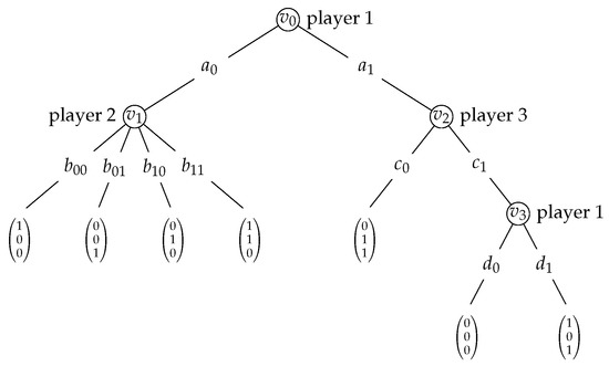
Figure 1. Extensive-form game of perfect information. The players are depicted besides the nodes at which they are active. Vertices are identified with histories, for instance, the root. $v_0$ with $( )$ vertex $v_3$ with $a_1{c}_1$ and the leaf node/terminal history labelled with $a_0{b}_{00}$ omitting parentheses and commas for better readability.

A strategy for player i in an extensive-form game is a function $s_i:{\mathcal{I}}_i\to A_i$ such that $s_i\left(I\right)\in A_I$ for all $I\in {\mathcal{I}}_i$. The set of strategies available to player i we then denote by $S_i$. A strategy profile is then a sequence $\mathbf{s}=(s_1,\cdots ,s_{\left|N\right|})$ of strategies, one for each player. Let $D=\{v_1,\cdots ,v_{\left|D\right|}\}$. Then, every strategy profile $\mathbf{s}=(s_1,\cdots ,s_{\left|N\right|})$ defines an action profile ${\mathbf{a}}^{\mathbf{s}}=(a_{v_1},\cdots ,a_{v_{\left|D\right|}})$ such that $a_v=s_i\left(\left[v\right]\right)$ and where i is a player who is active at v. Observe that a strategy profile $\mathbf{s}=(s_1,\cdots ,s_{\left|N\right|})$ also defines a unique path $w_0,\cdots ,w_k$ from the root $w_0$ to a leaf $w_k$ with history ${\mathbf{h}}^{\mathbf{s}}=(a_1,\cdots ,a_k)$ defined such that, for all $0\le i<k$, edge $(w_i,w_{i+i})$ is associated with action $a_i=s_i\left(\left[w_i\right]\right)$, where i is the player who is active at $w_i$. Finally, we have for each player i a utility function $u_i:S_1\times \cdots \times S_{\left|N\right|}\to \mathbb{R}$ associating each strategy profile $\mathbf{s}=(s_1,\cdots ,s_{\left|N\right|})$ with a real value such that $u_i\left(\mathbf{s}\right)=u_i^{{\mathbf{h}}_{\mathbf{s}}}$.

The players N of an extensive-form game, together with their strategies $S_i$ and their utilities $u_i$, induce a normal-form game $(N,{\left(S_i\right)}_{i\in N},{\left(u_i\right)}_{i\in N})$. Note that there may be multiple strategy profiles giving rise to the same terminal history, that is, it may well be that ${\mathbf{h}}^{\mathbf{s}}={\mathbf{h}}^{{\mathbf{s}}^{\prime }}$, even though $\mathbf{s}\ne {\mathbf{s}}^{\prime }$. Therefore, the size of this normal-form game may be exponential in the size of the underlying extensive-form game, if represented naively. This is because there are ${\prod }_{I\in \mathcal{I}}|A_I{|=O(\left|A\right|}^{\left|V\right|})$ strategy profiles, which are implicit in the definition of an extensive-form game: see Figure 2 for an illustration.

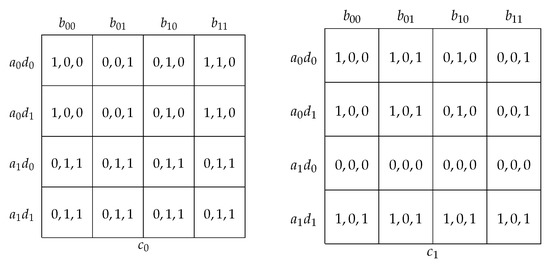
Figure 2. The strategic form game associated with the extensive-form game in Figure 1.

2.4. Boolean Circuits

In computer science, Boolean circuits are a well-established model for computing Boolean functions (cf., e.g., [6,7]). In this paper, we will make extensive use of them to concisely represent strategies and utility functions. We will here briefly review their definition, largely following Jukna’s exposition [7].

A k-ary Boolean function is a function $\beta :{\{0,1\}}^k\to \{0,1\}$, where we allow $k=0$. The base of a Boolean circuit is given by a set $B=\{{\beta }_1,\cdots ,{\beta }_k\}$ of Boolean functions. In this paper, we will restrict attention to the set of classical Boolean functions $B=\{\neg ,\wedge ,\vee \}$ (“not”, “or”, and “and”, respectively), which is known to be functionally complete (i.e., sufficient to define any Boolean function).

Formally, a Boolean circuit (or straight line program) on n variables $x_1,\cdots ,x_n$ over base B is given by a sequence of $t\ge n$ gates ${\gamma }_1,\cdots ,{\gamma }_t$. The first n gates are given by the variables, that is, ${\gamma }_1=x_1,\cdots ,{\gamma }_n=x_n$, and are also referred to as input gates. Another subset of gates is singled out as the set of output gates. Boolean formula over variables $x_1,\cdots ,x_n$ are thus represented by a Boolean circuit with only one output gate. Each subsequent gate ${\gamma }_i$ is the application of a k-ary Boolean function ${\beta }_i$ in the base B to k previous gates, that is, ${\gamma }_i={\beta }_i({\gamma }_{j_1},\cdots ,{\gamma }_{j_k})$, where $j_1,\cdots ,j_k<i$. The variables take values in $\{0,1\}$. Given values ${\alpha }_1,\cdots ,{\alpha }_n$ in $\{0,1\}$ for the variables $x_1,\cdots ,x_n$, one can inductively associate each gate with a value $\alpha \left({\gamma }_i\right)$ such that $\alpha \left(x_i\right)={\alpha }_i$, if $1\le i\le n$, and

$$\alpha \left({\beta }_i({\gamma }_{j_1},\cdots ,{\gamma }_{j_k})\right)= {\beta }_i(\alpha \left({\gamma }_{j_1}\right),\cdots ,\alpha \left({\gamma }_{j_k}\right)),$$

if $n<i\le t$. A Boolean circuit $\mathbb{C}$ given by ${\gamma }_1,\cdots ,{\gamma }_t$ on n variables $x_1,\cdots ,x_n$ and with m output gates ${\gamma }_{j_1},\cdots ,{\gamma }_{j_m}$ then computes the function ${\varphi }_{\mathbb{C}}:{\{0,1\}}^n\to {\{0,1\}}^m$ that, on values $\alpha =(b_1,\cdots ,b_n)$ for the input gates, yields ${\varphi }_{\mathbb{C}}\left(\alpha \right)=(\alpha \left({\gamma }_{j_1}\right),\cdots ,\alpha \left({\gamma }_{j_m}\right))$.

A Boolean circuit is commonly depicted as a directed acyclic graph $(V,E)$, with the gates as vertices, that is, $V=\{{\gamma }_1,\cdots ,{\gamma }_n\}$, and $({\gamma }_i,{\gamma }_j)\in E$ whenever ${\gamma }_i={\beta }_i({\gamma }_{j_1},\cdots ,{\gamma }_{j_k})$ and ${\gamma }_j={\gamma }_{j_{\ell }}$ for some $1\le \ell \le n$. For examples of Boolean circuits, also see Figure 3 and Figure 4, below.

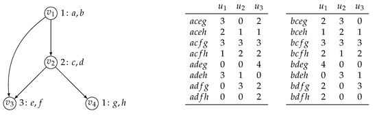
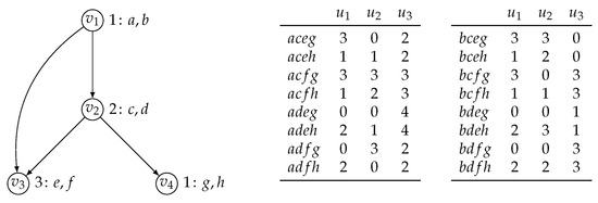
Figure 3. A simple example of a partial order game. On the left, the DAG, where each vertex v is labelled $i:x,y$, where i is the player active at the respective vertex and x and y are the actions available to i at v. On the right, the representation of the utility function which associates a numeric value with each action profile.

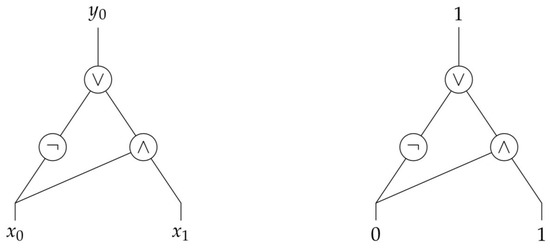
Figure 4. The Boolean circuit ${\mathbb{C}}_{f_{v_3}^{14}}$ representing strategy $f_{v_3}^{14}:A_{v_1}\times A_{v_2}\to A_{v_3}$ of Example 1. The value of $x_0$ represents the choice for a or b at $v_1$, the value of $x_1$ the choice for c or d at $v_2$, and the value of $y_0$ the choice for e or f at $v_3$. The local indices of a, c, and e are given by 0, and those of b, d, and f by 1. The instantiation on the right thus represents that $f_{v_3}^{14}\left(ad\right)=f$.

The size of a Boolean circuit given by gates ${\gamma }_1,\cdots ,{\gamma }_t$ on variables $x_1,\cdots ,x_n$ is given by the number $t-n$ of its gates minus the input gates. It is a well-established fact that the problem of computing ${\varphi }_{\mathbb{C}}\left(\alpha \right)$ for given values $\alpha \in {\{0,1\}}^n$ for $\mathbb{C}$’s variables, which is also known as the Circuit Value Problem or Circuit Evaluation Problem, is complete for $\mathrm{P}$ under uniform ${\mathrm{AC}}_0$-reductions, and therefore can be computed in polynomial time (see in [8], p. 59).

3. Partial Order Games

We now introduce the framework of partial order games. The basic idea is that, as in extensive form games, the game contains a number of decision nodes, which are partioned among the players. However, play in the game is not defined by a game tree. Instead, partial order games have a binary dependence relation over decision nodes. This dependence defines the information available to a player when it makes a choice. If a decision node v for player i is dependent on decision nodes $v_1,\dots ,v_k$, then this means that the information available to a strategy when making a choice at v is precisely the choices that were made at decision nodes $v_1,\dots ,v_k$. To play a partial order game, a player must choose a selection of strategies (we call them vertex strategies), one for each of their decision nodes. A strategy for a decision node v must select a choice for that decision node taking as input the choices that were made for the decision nodes $v_1,\dots ,v_k$ upon which it is dependent. In this way, we have an explicit representation of the information available when making a choice, in contrast to the use of information sets in extensive form games. Utilities in partial order games are not associated with individual nodes (as in extensive form games), but derive from the total profile of actions that were made.

Our usual way of thinking about extensive form games is as players alternating to make moves, working their way down the game tree to a leaf node; upon reaching a leaf node, the game is over. Thinking about games in this way naturally gives rise to a temporal order over choices in the game: a choice is made for the root node first, and then successive nodes in the game tree. Partial order games are more abstract than this. They induce only a partial temporal ordering over decision nodes: while the choices for $v_1,\dots ,v_k$ must strictly precede the choice for v if v is dependent on $v_1,\dots ,v_k$, it may well be that decision nodes are independent: if nodes v and $v^{\prime }$ are in disconnected components of the dependence graph, then we can say nothing about their temporal order.

Let us consider an example.

Example 1.

Consider the three-person partial order game depicted in Figure 3, with the directed acyclic graph it is based on given on the left. To the right of each vertex v, we have indicated the player$i_v$and the actions they have at their disposal at v. For instance, at vertex$v_2$, player 2 can choose among the actions c and d. If all players make a choice at their respective vertices, an action profile results, which then is associated with a utility value. For instance, if player 1 chooses a at$v_1$and h at$v_4$, player 2 chooses c at$v_2$, and player 3 chooses f at$v_3$, the action profile$(a,c,f,h)$(also denoted by$acfh$) results, yielding utility values of 1 to player 1, and 2 to players 2 and 3. The table on the right summarises the utilities the players get under the different action profiles that may be played. Note that in this game there are$2^4$possible action profiles.

The crucial feature of partial order games, however, is that the players can make their choices at a given vertex v depending on the choices the other players make at the parents of v. For instance, player 2 could adopt the strategy to play c at$v_2$, if player 1 chooses a at$v_1$, and plays d otherwise. Accordingly, player 2 has$2^2=4$strategies at their disposal at$v_2$. As$v_1$does not have any parents, player 1 has only two strategies at their disposal at$v_1$, but they have$2^2=4$strategies at$v_4$. Meanwhile, player 3 has$2^4=16$strategies at$v_3$. A strategy profile specifies a strategy for each player at each of their vertices. Accordingly, in this game there are$2\times 2^2\times 2^4\times 2^2=2^9=512$possible strategy profiles.

The number of strategy profiles clearly outnumber the number of action profiles. Still, every strategy profile induces a unique action profile. This relationship, however, is not generally injective, as multiple strategy profiles may induce the same action profile. Assume, for instance, that the players adopt the following strategies:

• player 1 chooses a at $v_1$;
• player 2 chooses c if player 1 plays a at v, and d, otherwise;
• player 3 chooses e if player 1 chooses a at $v_1$ and player 2 d at $v_2$, and f, otherwise; and
• player 4 chooses h independently of whether player 2 chooses c or d at $v_2$.

If this strategy profile is played, it can readily be seen that action profile$acfh$results, which we have already seen gives utilities 1, 2, and 2 to the players 1, 2, and 3, respectively.

We now proceed to our formal definition of partial order games, which enables the application of Nash equilibrium as well as the formulation of a natural backwards induction procedure later on. As before, let $N=\{1,\cdots ,n\}$ be a finite set of players. Then a partial order game on a directed acyclic graph $(V,E)$—the game’s dependency graph—associates each vertex v in V with a unique player in N, denoted by $i_v$, and a non-empty set of actions, denoted by $A_v$.

One player may be associated with multiple vertices, that is, it may very well be that $i_u=i_v$ even if $v\ne u$. We let $V_i$ denote the set of vertices associated with player i. We also say that player i is active at any vertex v in $V_i$. If E is also connected—that is, if $vEw$ or $wEv$ for all distinct v and w in V—we also refer to any partial order game based on it as a total-order game. As E is assumed to be acyclic, it follows that E is transitive in total order games. On the other end of the spectrum, we have partial order games on dependency graphs $(V,E)$ with $E=Ø$. This class of games we will also refer to as empty-order games.

Given a subset of $W=\{w_1,\cdots ,w_k\}$ of vertices, an action profile for W is a tuple ${\mathbf{a}}_W=(a_{w_1},\cdots ,a_{w_k})$ specifying one action $a_{w_j}$ for each vertex $w_j$. In our examples, we occasionally omit parentheses and commas, and write $a_{w_1}\cdots a_{w_k}$ for $(a_{w_1},\cdots ,a_{w_k})$. The set of action profiles for W we denote by ${\mathbf{A}}_W$. For the set $V=\{v_1,\cdots ,v_{\left|V\right|}\}$ of all vertices, we write write $\mathbf{a}=(a_{v_1},\cdots ,a_{v_{\left|V\right|}})$ for $a_V$ and refer to $\mathbf{a}$ simply as an action profile. We denote the set of action profiles by $\mathbf{A}=A_{v_1}\times \cdots \times A_{v_{\left|V\right|}}$. For a set $V_i=\{w_1,\cdots ,w_k\}$ of vertices at which a player i is active, we also write ${\mathbf{a}}_i=(a_{w_1},\cdots ,a_{w_k})$ for ${\mathbf{a}}_{V_i}$ and refer to ${\mathbf{a}}_i$ as an action profile for player i. We let ${\mathbf{A}}_i$ denote the set of actions profiles for a player i. For action profiles ${\mathbf{a}}_W=(a_{w_1},\cdots ,a_{w_k})$ and ${\mathbf{b}}_U=(b_{u_1},\cdots ,b_{u_m})$ for disjoint sets W and U, we denote by $({\mathbf{a}}_W,{\mathbf{b}}_U)$ the action profile $(a_{w_1},\cdots ,a_{w_k},b_{u_1},\cdots ,b_{u_m})$ for $W\cup U$. If $U=V\backslash W$ we also write $({\mathbf{a}}_W,{\mathbf{a}}_{-W})$ for $({\mathbf{a}}_W,{\mathbf{a}}_U)$, and if $U=V\backslash V_i$, we also write $({\mathbf{a}}_i,{\mathbf{a}}_{-i})$. Given a topological sorting $\tau =(v_1,\cdots ,v_{\left|V\right|})$, we define a $\tau$-history as a sequence of actions $\mathbf{h}=(a_{v_1},\cdots ,a_{v_k})$ in $A_{v_1}\times \cdots \times A_{v_{{}_k}}$ for some $1\le k\le \left|V\right|$. We stipulate the empty sequence of actions, denoted by $\left(\right)$, to be a $\tau$-history as well. For an action profile $\mathbf{a}=(a_{v_1},\cdots ,a_{v_{\left|V\right|}})$, we say that $\mathbf{h}=(b_{v_1},\cdots ,b_{v_k})$ is a history of $\mathbf{a}$ if $(b_{v_1},\cdots ,b_{v_k})=(a_{v_1},\cdots ,a_{v_k})$.

At each vertex v, player $i_v$ can make their choice of action dependent on the actions chosen at the parents of v. A (conditional) strategy at a vertex v, or vertex strategy, is therefore a function

$$f_v:A_{y_1}\times \cdots \times A_{y_k}\to A_v,$$

where $y_1,\cdots ,y_k$ are the parents of v. We say that $f_v$ is unconditional if it is constant, that is, if $f_v(a_1,\cdots ,a_k)=f_v(b_1,\cdots ,b_k)$ for all action profiles $\mathbf{a}=(a_1,\cdots ,a_k)$ and $\mathbf{b}=(b_1,\cdots ,b_k)$. In this case, for $a\in A_v$, we denote by $f_v^a$ the unconditional strategy at vertex v that maps every action profile of v’s parents to action a. We will sometimes identify unconditional strategies $f_v$ with the action $f_v(a_1,\cdots ,a_k)$ it specifies for each action profile $\mathbf{a}=(a_1,\cdots ,a_k)$ and write $\mathbf{a}=(a_{v_1},\cdots ,a_{v_{\left|V\right|}})$ for the profile of unconditional strategies ${\mathbf{f}}^{\mathbf{a}}=(f_{v_1}^{a_{v_1}},\cdots ,f_{v_{\left|V\right|}}^{a_{v_{\left|V\right|}}})$. Note that if vertex v has no parents, then $A_{u_1}\times \cdots \times A_{u_k}=\left\{\left(\right)\right\}$, where $\left(\right)$ is the empty tuple. Accordingly, $f_v$ determines a single choice among $A_v$, namely, $f_v\left(\left(\right)\right)$ in this case. By $F_v$ we denote the set of conditional strategies available at a vertex v.

By a strategy profile we then understand a profile $\mathbf{f}=(f_{v_1},\cdots ,f_{v_{\left|V\right|}})$ consisting of one conditional strategy for each vertex. For $\mathbf{f}=(f_{v_1},\cdots ,f_{v_{\left|V\right|}})$ a strategy profile and $W=\{w_1,\cdots ,w_k\}$ a subset of vertices in V, we let $f_W=(f_{w_1},\cdots ,f_{w_k})$ denote the partial profile that is like $\mathbf{f}$ but restricted to $W\subseteq V$. Let ${\mathbf{f}}^1=(f_{v_1}^1,\cdots ,f_{v_{\left|V\right|}}^1)$ through ${\mathbf{f}}^k=(f_{v_1}^k,\cdots ,f_{v_{\left|V\right|}}^k)$ be k strategy profiles and $\{X_1,\cdots ,X_k\}$ be a k-partition of the vertex set V. Then, $({\mathbf{f}}_{X_1}^1,\cdots ,{\mathbf{f}}_{X_k}^k)$ denotes the strategy profile $\mathbf{g}=(g_{v_1},\cdots ,g_{v_{\left|V\right|}})$ such that, for every vertex v in V, we have $g_v=f_v^j$, if $v\in X_j$.

A strategy for a player i is a profile ${\mathbf{f}}_{V_i}=(f_{v_1},\cdots ,f_{v_k})$ of vertex-strategies, where $V_i=\{v_1,\cdots ,v_k\}$, is the set of vertices at which player i is active. We generally denote ${\mathbf{f}}_{V_i}$ by ${\mathbf{f}}_i$, and the set of strategies available to player i by ${\mathbf{F}}_i$. For strategy profiles $\mathbf{f}=(f_{v_1},\cdots ,f_{v_{\left|V\right|}})$ and $\mathbf{g}=(g_{v_1},\cdots ,g_{v_{\left|V\right|}})$ and a player i, we also write $({\mathbf{f}}_{-i},{\mathbf{g}}_i)$ for the strategy profile $({\mathbf{f}}_{V\backslash V_i},{\mathbf{g}}_{V_i})$.

For every vertex v, a strategy profile $\mathbf{f}=(f_{v_1},\cdots ,f_{v_{\left|V\right|}})$ defines an action $a_v^{\mathbf{f}}$, the evaluation of $\mathbf{f}$ at v, recursively as follows:

$$\begin{array}{c}\hfill a_v^{\mathbf{f}}=\left\{\begin{array}{cc}{f}_v\left(\left(\right)\right)\hfill & \mathrm{if}\mathit{depth}\left(v\right)=0,\hfill \\ f_v(a_{u_1}^{\mathbf{f}},\cdots ,a_{u_k}^{\mathbf{f}})\hfill & \mathrm{if}\mathit{depth}\left(v\right)>0\mathrm{and}{u}_1,\cdots ,u_k\mathrm{are}\mathrm{the}\mathrm{parents}\mathrm{of}v.\hfill \end{array}\right.\end{array}$$

Observe that $a_v^{\mathbf{f}}$ is well defined because in a directed acyclic graph vertices with depth 0 exist and the parents of each vertex are of lower depth than the vertex itself. A strategy profile $\mathbf{f}=(f_{v_1},\cdots ,f_{v_{\left|V\right|}})$ can thus be seen to induce the action profile ${\mathbf{a}}^{\mathbf{f}}=(a_{v_1}^{\mathbf{f}},\cdots ,a_{v_{\left|V\right|}}^{\mathbf{f}})$. We also say that strategy profile $\mathbf{f}=(f_{v_1},\cdots ,f_{v_{\left|V\right|}})$sustains action profile $\mathbf{a}=(a_{v_1},\cdots ,a_{v_{\left|V\right|}})$ if $\mathbf{a}={\mathbf{a}}^{\mathbf{f}}$. We occasionally denote by $({\mathbf{a}}_W,{\mathbf{f}}_U)$ the action profile ${\mathbf{a}}^{\mathbf{g}}$ where $\mathbf{g}$ is the strategy profile $({\mathbf{f}}_W^{\mathbf{a}},{\mathbf{f}}_U)$ which specifies unconditional strategies for W. In other words, we have $(a_{v_1},\cdots ,a_{v_k},f_{v_{k+1}},\cdots ,f_{v_{\left|V\right|}})$ denote the action profile that results if on $v_1$ through $v_{v_k}$ actions $a_{v_1},\cdots ,a_{v_k}$ are played, and at vertices $a_{v_{k+1}}$ through $a_{v_{\left|V\right|}}$ the strategies $f_{v_{k+1}}$ through $f_{v_{\left|V\right|}}$.

Note the difference between actions and action profiles on the one hand, and strategies and strategy profiles on the other. Every strategy profile induces a unique action profile, whereas the same action profile may be induced by different strategy profiles. In an important sense, the action profiles are the outcomes of the game.

Therefore, we take the set of action profiles of a partial order game as its set of outcomes, over which the players’ preferences are defined. Each player’s preferences over the action profiles are given by a real-valued utility function $u_i:\mathbf{A}\to \mathbb{R}$, where we assume that player istrictly prefers action profile $\mathbf{a}=(a_{v_1},\cdots ,a_{v_{\left|V\right|}})$ to action profile $\mathbf{b}=(b_{v_1},\cdots ,b_{v_{|}V|})$ whenever $u_i\left(\mathbf{a}\right)>u_i\left(\mathbf{b}\right)$. We extend utility functions $u_i$ to strategy profiles $\mathbf{f}$, and write $u_i\left(\mathbf{f}\right)$ for $u_i\left({\mathbf{a}}^{\mathbf{f}}\right)$. To fix concepts and notation, we consider Example 1 once more.

Example 1 (cont’d).

Consider the game in Figure 3. At vertices $v_1$, $v_2$, and $v_4$, we have the following strategies:

$$\begin{array}{ccccc}\underline{F_{v_1}\hspace{1em}\left(\right)}& & \underline{F_{v_2}\hspace{1em}a\hspace{1em}b}& & \underline{F_{v_4}\hspace{1em}c\hspace{1em}d}\\ f_{v_1}^1\hspace{1em}a& & f_{v_2}^1\hspace{1em}c\hspace{1em}c& & f_{v_4}^1\hspace{1em}g\hspace{1em}g\\ \underline{f_{v_1}^2\hspace{1em}b}& & f_{v_2}^2\hspace{1em}c\hspace{1em}d& & f_{v_4}^2\hspace{1em}g\hspace{1em}h\\ & & f_{v_2}^3\hspace{1em}d\hspace{1em}c& & f_{v_4}^3\hspace{1em}h\hspace{1em}g\\ & & \underline{f_{v_2}^4\hspace{1em}d\hspace{1em}d}& & \underline{f_{v_4}^4\hspace{1em}h\hspace{1em}h}\end{array}$$

At vertex $v_3$, moreover, we have $2^4$ strategies, illustrating the exponential blowup that results from strategies being represented explicitly.

$$\begin{array}{ccccccc}\underline{F_3\hspace{1em}ac\hspace{1em}ad\hspace{1em}bc\hspace{1em}bd}& & \underline{\hspace{1em}\hspace{1em}ac\hspace{1em}ad\hspace{1em}bc\hspace{1em}bd}& & \underline{\hspace{1em}\hspace{1em}ac\hspace{1em}ad\hspace{1em}bc\hspace{1em}bd}& & \underline{\hspace{1em}\hspace{1em}ac\hspace{1em}ad\hspace{1em}bc\hspace{1em}bd}\\ f_{v_3}^1\hspace{1em} e\hspace{1em} e\hspace{1em} e\hspace{1em} e& & f_{v_3}^5\hspace{1em} e\hspace{1em} f\hspace{1em} e\hspace{1em} e& & f_{v_3}^9\hspace{1em} f\hspace{1em} e\hspace{1em} e\hspace{1em} e& & f_{v_3}^{13}\hspace{1em} f\hspace{1em} f\hspace{1em} e\hspace{1em} e\\ f_{v_3}^2\hspace{1em} e\hspace{1em} e\hspace{1em} e\hspace{1em} f& & f_{v_3}^6\hspace{1em} e\hspace{1em} f\hspace{1em} e\hspace{1em} f& & f_{v_3}^{10}\hspace{1em} f\hspace{1em} e\hspace{1em} e\hspace{1em} f& & f_{v_3}^{14}\hspace{1em} f\hspace{1em} f\hspace{1em} e\hspace{1em} f\\ f_{v_3}^3\hspace{1em} e\hspace{1em} e\hspace{1em} f\hspace{1em} e& & f_{v_3}^7\hspace{1em} e\hspace{1em} f\hspace{1em} f\hspace{1em} e& & f_{v_3}^{11}\hspace{1em} f\hspace{1em} e\hspace{1em} f\hspace{1em} e& & f_{v_3}^{15}\hspace{1em} f\hspace{1em} f\hspace{1em} f\hspace{1em} e\\ \underline{f_{v_3}^4\hspace{1em} e\hspace{1em} e\hspace{1em} f\hspace{1em} f}& & \underline{f_{v_3}^8\hspace{1em} e\hspace{1em} f\hspace{1em} f\hspace{1em} f}& & \underline{f_{v_3}^{12}\hspace{1em} f\hspace{1em} e\hspace{1em} f\hspace{1em} f}& & \underline{f_{v_3}^{16}\hspace{1em} f\hspace{1em} f\hspace{1em} f\hspace{1em} f}\end{array}$$

The (conditional) strategy profile $\mathbf{f}=(f_{v_1}^1,f_{v_2}^3,f_{v_3}^8,f_{v_4}^2)$, then, for instance, yields the evaluation ${\mathbf{a}}^{\mathbf{f}}=(a_{v_1}^{\mathbf{f}},a_{v_2}^{\mathbf{f}},a_{v_3}^{\mathbf{f}},a_{v_4}^{\mathbf{f}})=(a,d,f,h)$ as

$$\begin{array}{cccc}\hfill a_{v_1}^{\mathbf{f}}& =f_{v_1}^1\left(\left(\right)\right)=a\hfill & \hfill a_{v_2}^f& =f_{v_2}^3\left(a_{v_1}^{\mathbf{f}}\right)=f_{v_2}^3\left(a\right)=d\hfill \\ \hfill a_{v_3}^f& =f_{v_3}^8(a_{v_1}^{\mathbf{f}},a_{v_2}^{\mathbf{f}})=f_{v_3}^8(a,d)=f\hfill & \hfill a_{v_4}^f& =f_{v_4}^2\left(a_{v_2}^{\mathbf{f}}\right)=f_{v_4}^2\left(d\right)=h\hfill \end{array}$$

Accordingly, the utilities on this profile $\mathbf{f}=(f_{v_1}^1,f_{v_2}^3,f_{v_3}^8,f_{v_4}^2)$ for these three players are therefore determined by the action profile $adfh$. Hence, $u_1\left(f\right)=0$, $u_2\left(f\right)=0$, and $u_3\left(f\right)=2$.

With the players N, their conditional strategies ${\mathbf{F}}_i$, and their preferences $u_i:\mathbf{F}\to \mathbb{R}$ over strategy profiles, a partial order game on a directed acyclic graph $(V,E)$ can thus be seen to define immediately a game in normal-form $(N,{\left({\mathbf{F}}_i\right)}_{i\in N},{\left(u_i\right)}_{i\in N})$ (cf., Section 2.2, above). Accordingly, partial order games are directly amenable to game-theoretical analysis using the usual solution concepts, in particular, Nash equilibrium.

Conversely, every normal-form game $(N,{\left(S_i\right)}_{i\in N},{\left(u_i\right)}_{i\in N})$ can be seen as a partial order game on the same set N of players. Its dependency graph is then given by $(N,Ø)$, associating with vertex $i\in N$, player $i\in N$ and strategy set $S_i$. Identifying each unconditional strategy $f_i$ with $f_i\left(\left(\right)\right)=s_i$ in $S_i$, we adopt the utility functions $u_i$ unaltered for the utility functions of the partial order game.

3.1. Concise Representations for Strategies, Profiles, and Utilities

The transformation from partial order games to normal-form games comes at the cost of an exponential blowup. Observe that in the definition of partial order games, the sets of action profiles and strategy profiles are defined implicitly. Given a partial order game on a directed acyclic graph $(V,E)$ with a set of players N and actions $A=A_{v_1}\cup \cdots \cup A_{v_{\left|V\right|}}$, the number of action profiles $\mathbf{a}=(a_{v_1},\cdots ,a_{v_{\left|V\right|}})$ is bounded by $O\left(\right|A{|}^{\left|V\right|})$, and so is the number of unconditional strategy profiles ${\mathbf{f}}^{\mathbf{a}}=(f_{v_1}^{a_{v_1}},\cdots ,f_{v_{\left|V\right|}}^{a_{v_{\left|V\right|}}})$. By contrast, the number of both conditional strategies and the number of conditional strategy profiles are bounded by $O\left(\right|A{|}^{\left(\right|A{|}^{\left|V\right|})})$. It is also worth observing that the size of both a conditional strategy f and a profile $\mathbf{f}=(f_{v_1},\cdots ,f_{v_{\left|V\right|}})$ of conditional strategies is bounded by $O\left(\right|A{|}^{\left|V\right|})$.

Even though the dependency graph allows a concise representation of the strategies and strategy profiles in a partial order game, they remain large objects. It is therefore desirable to have concise representations of action profiles, utility functions, strategies, and strategy profiles. To this end, we take recourse to Boolean circuits, a formalism well established in theoretical computer science (see Section 2.4). We first show how action profiles, utility functions, and strategy profiles can be represented concisely by Boolean circuits. We then prove two lemmas that will be useful for our later complexity proofs in Section 5 and Section 7.

When representing partial order games concisely, we assume that for distinct vertices v and w the action sets $A_v$ and $A_w$ are disjoint. Having assumed $A_v$ to be non-empty for each vertex v, it thus follows that $\left|V\right|\le \left|A\right|$. For ease of presentation, we also assume that $|A_v|$ is an integer power of 2 for each vertex v. In this section, we assume that for each vertex v, the elements of set $A_v$ are enumerated as $a_0,\cdots ,a_{|A_v|-1}$, thus associating each action $a_k$ with a unique local index k at v. Let $\mathit{bin}\left(k\right)$ denote the binary representation of the local index k, using exactly ${log}_2\left|A_v\right|$ digits. Thus, if $|A_v|=16$, we have $\mathit{bin}\left(3\right)=0011$.

Let v be a vertex with parents $u_1,\cdots ,u_k$. We then represent a strategy $f_v:A_{u_1}\times \cdots \times A_{u_k}\to A_v$ by a Boolean circuit ${\mathbb{C}}_{f_v}$ with ${log}_2|A_{u_1}|+\cdots +{log}_2\left|A_{u_k}\right|$ input gates and ${log}_2\left|A_v\right|$ output gates. For an action profile $\mathbf{a}=(a_{u_1},\cdots ,a_{u_k})$ in $A_{u_1}\times \cdots \times A_{u_k}$ and $a_v$ an action in $A_v$, we then have that $f_v(a_{u_1},\cdots ,a_{u_k})=a_v$ if and only if on input $\mathit{bin}\left(j_1\right)\cdots \mathit{bin}\left(j_k\right)$ the circuit ${\mathbb{C}}_{f_v}$ evaluates to outputs $\mathit{bin}\left(i\right)$, where $j_1,\cdots ,j_k$ and i, are the local indices of $a_{v_1},\cdots ,a_{v_k}$, and $a_v$ at their respective vertices. As ${\mathbb{C}}_{f_v}$ can be seen as combining ${log}_2\left|A_v\right|$ Boolean functions in ${log}_2|A_{u_1}|+\cdots +{log}_2\left|A_{u_k}\right|$ variables and ${log}_2|A_{u_1}|+\cdots +{log}_2|A_{u_k}|\le |A|$, we may assume that the circuit ${\mathbb{C}}_{f_v}$ is of size at most exponential in $\left|A\right|$. More precisely, we may assume that the size of ${\mathbb{C}}_{f_v}$ is $\mathsf{\Theta }(\frac{2^{\left|A\right|}}{\left|A\right|})$ [9,10].

Example 2.

For an example, see Figure 4, which depicts the Boolean circuit ${\mathbb{C}}_{f_{v_3}^{14}}$ for strategy $f_{v_3}^{14}:A_{v_1}\times A_{v_2}\to A_{v_3}$ in Example 1, given by

$$f_{v_3}^{14}\left(\mathbf{a}\right)=\left\{\begin{array}{cc}e\hfill & \mathrm{if}\mathbf{a}=bc,\hfill \\ f\hfill & \mathrm{otherwise}.\hfill \end{array}\right.$$

Recall that $A_{v_1}=\{a,b\}$, $A_{v_2}=\{c,d\}$, and $A_{v_3}=\{e,f\}$. Let the local indices of a, c, and e be given by 0, and those of b, d, and f by 1. As $|A_{v_1}| = |A_{v_2}| = |A_{v_3}| = 2$, any action profile $\mathbf{a}\in A_{v_1}\times A_{v_2}$ can be represented by two Boolean variables $x_0$ and $x_1$, where the value of $x_0$ represents the choice for a or b at $v_1$, the value of $x_1$ the choice for c or d at $v_2$. For instance, the action profile $ad\in A_{v_1}\times A_{v_2}$ can thus be represented by setting $x_0$ to 0 and $x_1$ to 1. For these values the circuit ${\mathbb{C}}_{f_{v_3}^{14}}$ evaluates to 1, which corresponds to $f_{v_3}^{14}\left(ad\right)=f$ and as depicted in Figure 4.

Observe that an unconditional strategy $f_v^a$ at a vertex v with parents $u_1,\cdots ,u_k$, which maps every profile $(a_{u_1},\cdots ,a_{u_k})$ invariably to action a in $A_v$, is represented by a Boolean circuit ${\mathbb{C}}_{f_v^a}$ of size at most polynomial in $\left|A\right|$. The circuit ${\mathbb{C}}_{f_v^a}$ will still have ${\sum }_{1\le m\le k}{log}_2\left|A_{u_m}\right|$ inputs and ${log}_2\left|A_v\right|$ outputs, but will involve only one ⊥-gate and one ⊤-gate. Let j be the local index of a at v and $\mathit{bin}\left(j\right)=b_1,\cdots ,b_{{log}_2\left|A_v\right|}$. Then, for $1\le \ell \le {log}_2\left|A_v\right|$, connect the ⊥-gate with output $y_{\ell }$, if $b_{\ell }=0$, and the ⊤-gate with output $y_{\ell }$, if $b_{\ell }=1$.

Similarly, a rational-valued utility function $u_i:A_{v_1}\times \cdots \times A_{v_{\left|V\right|}}\to \mathbb{Q}$ can be represented by a Boolean circuit ${\mathbb{C}}_{u_i}$. This circuit will have ${\sum }_{v\in V}{log}_2\left|A_v\right|$ inputs and outputs $y_1,\cdots ,y_k,z_1,\cdots ,z_m$. Moreover, for $(a_{v_1},\cdots ,a_{v_{\left|V\right|}})$ an action profile in $A_{v_1}\times \cdots \times A_{v_{\left|V\right|}}$ with local indices $j_1,\cdots ,j_{\left|V\right|}$ at their respective vertices, we have $u_i(a_{v_1},\cdots ,a_{v_{\left|V\right|}})=\frac{n}{d+1}$ if and only if on input $\mathit{bin}\left(j_1\right),\cdots ,\mathit{bin}\left(j_{\left|V\right|}\right)$ the circuit ${\mathbb{C}}_{u_i}$ yields $\mathit{bin}\left(n\right)$ for outputs $y_1,\cdots ,y_k$ and $\mathit{bin}\left(d\right)$ for outputs $z_1,\cdots ,z_m$ (Observe that if $u_i(a_{v_1},\cdots ,a_{v_{\left|V\right|}})$ is a positive integer, the outputs $z_1,\cdots ,z_m$ can be dispensed with, as ${\sum }_{x\in Ø}x=0$ and $d={\sum }_{1\le j\le m}{z}_j·2^j$). Again, as $|A_{u_1}|+\cdots +|A_{u_k}|\le |A|$, we may assume that any such circuit ${\mathbb{C}}_{u_i}$ will be of size at most exponential in $\left|A\right|$.

Example 3.

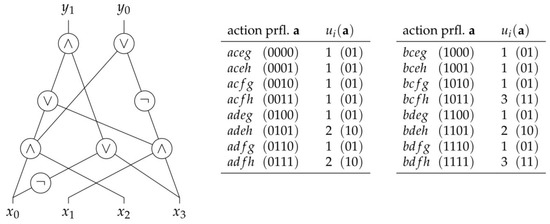
Figure 5 illustrates how a utility function $u_i:A_{v_1}\times A_{v_2}\times A_{v_3}\times A_{v_4}\to \mathbb{R}$ for a player i in the game of Example 1 is represented by a Boolean circuit. The utility function $u_i$ is depicted on the right. We assume that the local indices of a, c, e, and g be given by 0, and those of b, d, f, and h by 1. As $|A_{v_1}| = |A_{v_2}| = |A_{v_3}| = |A_{v_4}| = 2$, an action profile $\mathbf{a}$ in $A_{v_1}\times A_{v_2}\times A_{v_3}\times A_{v_4}$ is thus given by means of an assignment to four Boolean variables $x_0$, $x_1$, $x_2$, and $x_4$, representing the choices at the vertices $v_1$, $v_2$, $v_3$, and $v_4$, respectively. For instance, action profile $acfh$ is represented by setting variables $x_0$ and $x_1$ to 0, and variables $x_2$ and $x_3$ to 1, which can thus also be denoted by the binary string 0011. Evaluating the circuit for these values, we find that $y_1$ is set to 0 and $y_0$ to 1. This corresponds to $u_i\left(acfh\right)=1$ and $\mathit{bin}\left(1\right)=01$. Observe that the Boolean circuit can be evaluated in time polynomial in its size and that it is exponentially smaller than the explicit tabelling of the utility function on the right.

Figure 5. The Boolean circuit on the left represents the utility function $u_i$ on the right for a player i over the action profiles of the game in Example 1. The binary representations of action profiles and numerical values are depicted in parentheses.

We conclude this section by showing two useful lemmas. The first establishes that, even if a conditional strategy profile $\mathbf{f}=(f_{v_1},\cdots ,s_{v_{\left|V\right|}})$ is represented as a Boolean circuit, the action profile ${\mathbf{a}}^{\mathbf{f}}=(a_{v_1},\cdots ,a_{v_{\left|V\right|}})$ that $\mathbf{f}$ gives rise to, can be computed in polynomial time.

Lemma 1.

Let $\mathbf{f}=(f_{v_1},\cdots ,f_{v_{\left|V\right|}})$ be a conditional strategy profile represented by Boolean circuits ${\mathbb{C}}_{f_{v_1}},\cdots ,{\mathbb{C}}_{f_{v_{\left|V\right|}}}$. Then, the action profile ${\mathbf{a}}^{\mathbf{f}}=(a_{v_1}^{\mathbf{f}},\cdots ,a_{v_{\left|V\right|}}^{\mathbf{f}})$ can be computed in polynomial time.

Proof Sketch.

Proceeding inductively, find for every vertex v the action $a_v^{\mathbf{f}}$ as follows. For vertices v of depth 0, the Boolean circuit ${\mathbb{C}}_{f_v}$ should give the local index in binary of action $a_v^{\mathbf{f}}$ at v, and therewith, $a_v^{\mathbf{f}}$ immediately. For a vertex v of a strictly positive depth with parents $u_1,\cdots ,u_k$, we may assume that the local indices in binary $\mathit{bin}\left(j_{u_1}\right),\cdots ,\mathit{bin}\left(j_{u_k}\right)$ of $a_{u_1}^{\mathbf{f}},\cdots ,a_{u_k}^{\mathbf{f}}$ can be computed in polynomial time. As the evaluation problem for Boolean circuits is solvable in polynomial time, the circuit ${\mathbb{C}}_{f_v}$ for inputs $\mathit{bin}\left(j_{u_1}\right),\cdots ,\mathit{bin}\left(j_{u_k}\right)$ can also be evaluated in polynomial time, providing us with the local index of $f_v(a_{u_1}^{\mathbf{f}},\cdots ,a_{u_k}^{\mathbf{f}})$ at v in binary, which gives us the result. □

Lemma 2.

Let $\mathbf{f}=(f_{v_1},\cdots ,f_{v_{\left|V\right|}})$ be a conditional strategy profile represented by Boolean circuits ${\mathbb{C}}_{f_{v_1}},\cdots ,{\mathbb{C}}_{f_{v_{\left|V\right|}}}$, and $u_i:A_{v_1}\times \cdots \times A_{v_{\left|V\right|}}\to \mathbb{Q}$ be a utility function represented by a Boolean circuit ${\mathbb{C}}_{u_i}$. Then, $u_i\left(\mathbf{f}\right)$ can be computed in polynomial time.

Proof Sketch.

Thanks to Lemma 1, we can compute the action profile ${\mathbf{a}}^{\mathbf{f}}=(a_{v_1}^{\mathbf{f}},\cdots ,a_{v_{\left|V\right|}}^{\mathbf{f}})$ in polynomial time. Let $j_1,\cdots ,j_{\left|V\right|}$ be the local indices of $a_{v_1}^{\mathbf{f}},\cdots ,a_{v_{\left|V\right|}}^{\mathbf{f}}$ at their respective vertices. Using $\mathit{bin}\left(j_1\right),\cdots ,\mathit{bin}\left(j_{\left|V\right|}\right)$ as inputs for the circuit ${\mathbb{C}}_{u_i}$, we obtain the binary encoding of $u_i(a_{v_1}^{\mathbf{f}},\cdots ,a_{v_{\left|V\right|}}^{\mathbf{f}})$. As the evaluation problem for Boolean circuits is solvable in polynomial time, this suffices for the result. □

4. Related Game-Theoretic Models

In this section, we explore the interrelations between partial order games and four related game-theoretic models: partial order Boolean games, Multi-Agent Influence Diagrams (MAIDs), concurrent games as event structures, and extensive-form games.

4.1. Boolean Games and Partial Order Boolean Games

A special class of partial order games, referred to as partial order Boolean games, was introduced in [1]. Partial order Boolean games extend Boolean games [11,12,13,14,15], where for a set $\mathsf{\Phi }$ of propositional variables, each player i exercises unique control over the truth-values assigned to a subset ${\mathsf{\Phi }}_i$ of variables and aims to satisfy a goal formula ${\gamma }_i$ over $\mathsf{\Phi }$. Partial order Boolean games are Boolean games enriched with a dependency graph on $\mathsf{\Phi }$. To avoid confusion, we will write $v_p$ for the propositional variable p when it occurs in the role of a vertex in the dependency graph. The player i associated with a vertex $v_p$ coincides with the player controlling p in the Boolean game, and i can make their choice of truth-value for p depend on the values assigned to the propositional variables $q_1,\cdots ,q_k$ if $v_{q_1},\cdots ,v_{q_k}$ are the parents of $v_p$ in the dependency graph. In a Boolean game, such dependencies do not exist. Thus, Boolean games can be seen as a special class of partial order Boolean games. The class where the dependency graph does not have any edges but can be expressed by $(\mathsf{\Phi },Ø)$.

Clearly, every partial order Boolean game $(N,\mathsf{\Phi },{\mathsf{\Phi }}_1,\cdots ,{\mathsf{\Phi }}_n,{\gamma }_1,\cdots ,{\gamma }_n,D)$, where $D=(\mathsf{\Phi },E)$ is a dependency graph on $\mathsf{\Phi }$, defines a partial order game with the same set of players N and the same dependency graph, where player i is associated with vertex $v_p$ if and only if $p\in {\mathsf{\Phi }}_i$. At vertex $v_p$, the player i associated with $v_p$ has two actions at their disposal: setting p to true (p) and setting p to false ($\overline{p}$). We will assume that the local index of action p at vertex $v_p$ is 1 and that that of action $\overline{p}$ at $v_p$ is 0.

In a partial order Boolean game, an individual strategy at vertex $v_p$, controlled by i, is represented by a so-called choice equation of the form $p:\phi (q_1,\cdots ,q_k)$, where $v_{q_1},\cdots ,v_{q_k}$ are the parents of $v_p$ and $\phi (q_1,\cdots ,q_k)$ is a propositional logic formula over $q_1,\dots ,q_k$, with the interpretation that i sets p to true if $\phi (q_1,\cdots ,q_k)$ evaluates to true given the decisions made for $q_1,\cdots ,q_k$ at, $v_{q_1},\cdots ,v_{q_k}$, and to false otherwise. Thus a choice equation $p:\phi (q_1,\cdots ,q_k)$ defines an individual strategy $f_{v_p}:\{q_1,{\overline{q}}_1\}\times \cdots \times \{q_k,{\overline{q}}_k\}\to \{p,\overline{p}\}$ at vertex $v_p$. This strategy, moreover, can be represented by a Boolean circuit ${\mathbb{C}}_{f_{v_p}}$ for the Boolean function ${\beta }_{\phi }:{\{0,1\}}^k\to \{0,1\}$ expressed by the formula $\phi$. We may assume that the circuit ${\mathbb{C}}_{f_{v_p}}$ is of size at most polynomial in the size of the choice equation $p:\phi (q_1,\cdots ,q_k)$ and that it has exactly k inputs and one output. We may furthermore assume that the circuit ${\mathbb{C}}_{f_{v_p}}$ can be obtained in time polynomial in the size of $\phi$ from $p:\phi (q_1,\cdots ,q_k)$.

Similar considerations apply to the representation of the players’ utility functions. In partial order Boolean games, the preferences of each player i are represented by a goal formula ${\gamma }_i$ in the propositional language over $\mathsf{\Phi }$. Every action profile $\mathbf{a}=(a_{v_{p_1}},\cdots ,a_{v_{p_{\left|\mathsf{\Phi }\right|}}})$ of a Boolean partial order game defines a valuation ${\alpha }_{\mathbf{a}}:\mathsf{\Phi }\to \{0,1\}$ and yields player i utility 1 if ${\alpha }_{\mathbf{a}}$ satisfies ${\gamma }_i$, and utility 0 otherwise. The Boolean function ${\beta }_{{\gamma }_i}:{\{0,1\}}^{\left|\mathsf{\Phi }\right|}\to \{0,1\}$ expressed by ${\gamma }_i$ can be represented by a Boolean circuit ${\mathbb{C}}_{{\gamma }_i}$ with at most $\left|\mathsf{\Phi }\right|$ inputs and exactly one output. As at every vertex $v_p$, the assigned player has exactly two actions at their disposal and utility values are integers, we find that ${\mathbb{C}}_{{\gamma }_i}$ is exactly of the form suggested for the representation of players’ utilities in partial order games in the previous section. Moreover, ${\mathbb{C}}_{{\gamma }_i}$ will be of size at most exponential in $\left|\mathsf{\Phi }\right|$ and of size polynomial in ${\gamma }_i$. We may furthermore assume that the circuit ${\mathbb{C}}_{f_{{\gamma }_i}}$ can be obtained from ${\gamma }_i$ in polynomial time.

4.2. Multi-Agent Influence Diagrams (MAIDs)

Multi-agent Influence Diagrams (MAIDS) were proposed in [2,3] and later extended from a game-theoretic perspective in [16]. MAIDs trace their origins to Bayesian Networks (cf., [17]) and influence diagrams, a decision theoretic extension of Bayesian networks proposed by Howard and Matheson [18].

Like partial order games, MAIDs involve a finite set $\mathcal{A}=\{a_1,\cdots ,a_n\}$ of agents and are defined in directed acyclic graphs, where three different types of vertices are distinguished: a set of chance nodes $\mathcal{X}$, a set of decision nodes ${\mathcal{D}}_a$ for each agent a in $\mathcal{A}$, and a set of utility nodes ${\mathcal{U}}_a$ also for each agent a. In line with the Bayesian network literature, every vertex is taken to be a random variable X with possible values in a finite domain $\mathit{dom}\left(X\right)$. It is generally assumed that utility nodes cannot be parents of other nodes, and that their domain is a finite set of real numbers. (Hammond et al. [16] relax this condition, and also allow utility nodes to have outgoing edges.)

The values any variable in a MAID can take may depend on the values assumed by that variable’s parents in the DAG. This is very much in line with how a choice of action at a node may depend on the decisions taken at parent nodes in partial order games. In the MAIDs framework, the parents of a decision node X are denoted by $\mathit{Pa}\left(X\right)$ and an instantiation, commonly denoted by $\mathbf{pa}$, for $\mathit{Pa}\left(X\right)=\{Y_1,\cdots Y_k\}$ defines a value from the domain of each of these variables, that is, $\mathbf{pa}\in \mathit{dom}\left(Y_1\right)\times \cdots \times \mathit{dom}\left(Y_k\right)$. A conditional probabilistic distributions (CPD) for a decision or utility node X now assigns a probability $P\left(X\right|\mathbf{pa})$ for each instantiation $\mathbf{pa}$ of $\mathit{Pa}\left(X\right)$, and a decision rule defines a conditional probabilistic distribution for one particular decision variable. Sometimes it is required that CPDs for utility nodes be deterministic, arguing that all of the stochasticity should be subsumed into chance variables. This convention, however, is not universally adopted in the literature on MAIDS. We refer to the work in [19] for a good in-depth study. On this basis, a strategy ${\delta }_a$ for an agent a defines a conditional probability distribution for each decision variable D in ${\mathcal{D}}_a$. A strategy profile is then a tuple $({\delta }_{a_1},\cdots ,{\delta }_{a_n})$ of strategies, one for each agent. Given a strategy profile $({\delta }_{a_1},\cdots ,{\delta }_{a_n})$, the MAID reduces to a Bayesian network, and as such defines a joint probability distribution $P_{{\delta }_{a_1},\cdots ,{\delta }_{a_n}}$ over all of its variables. Accordingly, every agent a can be assigned a expected utility defined as follows:

$${\mathbb{E}}_a({\delta }_{a_1},\cdots ,{\delta }_{a_n})=\sum _{U\in {\mathcal{U}}_a}\sum _{x\in \mathit{dom}\left(U\right)}{P}_{{\delta }_{a_1},\cdots ,{\delta }_{a_n}}(U=x)·x.$$

With players, their strategies, and their utilities being defined, a MAID defines a strategic-form game, and is amenable to analysis by the usual game-theoretic solution concepts.

It is not hard to see how every partial order game can be seen as a MAID without chance variables, with ‘hidden’ utility nodes, and only allowing for deterministic decision rules. Formally, let $N=\{1,\cdots ,n\}$ be the set of players; $V_1,\cdots ,V_n$ be the sets of nodes assigned to the players 1 through n, respectively; $(V,E)$ be a directed acyclic graph with $V=V_1\cup \cdots \cup V_n$; and $u_1,\cdots ,u_n$ be utility functions for the players 1 through n. Then, the partial order game defined from this can be seen as a MAID with set of agents $\mathcal{A}=N$ and decision variables $V_1,\cdots ,V_n$ such that $\mathit{dom}\left(V_v\right)=A_v$ for all vertices v in V. There are no chance variables, and one utility variable $U_i$ for each player i that is a child of all decision nodes. The MAID’s partial order is then given by $(V^{\prime },E^{\prime })$ where $V^{\prime }=V\cup \{U_1,\cdots ,U_n\}$ and $E^{\prime }=E\cup V\times \{U_1,\cdots ,U_n\}$. Thus, the instantiations of the parents of each utility variable, the set of instantiations of all decision variables, corresponds to the set of all action profiles of the partial order game. Each of these instantiations $(a_{v_1},...a_{v_{\left|V\right|}})$, in turn, corresponds to a deterministic strategy profile $({\delta }_1,...,{\delta }_n)$ in the MAID, which allows us to complete the model by setting ${\mathbb{E}}_i\left(({\delta }_1,...,{\delta }_n)\right)=u_i((a_{v_1},...a_{v_{\left|V\right|}}))$.

4.3. True Concurrency and Games as Event Structures

Event structures [20] are the so-called “true concurrency” analogue of trees: just as transition systems unfold to trees, so some models of true concurrency, such as Petri nets and asynchronous transition systems, unfold to event structures [21]. Similarly, in the same way that sequential games can be represented by trees, certain concurrent games can be represented by event structures—where plays in this much more general setting determine partial instead of total orders of moves; cf., see in [22,23].

An event structure is a triple $(E,\le ,\mathrm{Con})$, consisting of a set E of events that are partially ordered by ≤, the causal dependency relation, and a nonempty consistency relation Con over finite subsets of E, which satisfy four conditions:

1.

$\{e^{\prime }:e^{\prime }\le e\mathrm{is}\mathrm{finite}\mathrm{for}\mathrm{all}e\in E\}$,

2.

$\left\{e\right\}\in \mathrm{Con}\mathrm{for}\mathrm{all}e\in E$,

3.

$Y\subseteq X\in \mathrm{Con}\mathrm{implies}Y\in \mathrm{Con}$, and

4.

$X\in \mathrm{Con}\mathrm{and}e\le e^{\prime }\in X\mathrm{implies}X\cup \left\{e\right\}\in \mathrm{Con}$.

The states of an event structures E are called configurations, denoted by $\mathcal{C}\left(E\right)$, and consist of those subsets $x\subseteq E$ which are both

• consistent:$\forall X\subseteq x.X\mathrm{is}\mathrm{finite}\mathrm{implies}X\in \mathrm{Con}$; and
• down-closed:$\forall e,e^{\prime }.e^{\prime }\le e\in x\mathrm{implies}{e}^{\prime }\in x$.

Configurations can be finite or infinite. Concurrency, then, is naturally modelled as follows: two events, say e and $e^{\prime }$, which are both consistent and incomparable with respect to causal dependency are seen as concurrent, and assumed to be independent in that they can happen in parallel. In a game-theoretic context, it also means that such two events can be played or executed in parallel.

In the context of concurrent games as event structures, we consider only two players, named Player (the system) and Opponent (the environment), who own disjoint sets of events which they can play (execute). They do so asynchronously in an attempt to reach a state in their “winning set” of configurations. In these games, players are allowed to execute an event, say e, only if all events on which e causally depends have been executed. In this setting, events do not have a Boolean or otherwise interpretation; they are simply available actions that a player can execute—and informally are intended to represent observable events in a computer system. The Nash equilibrium of concurrent games as event structures have been studied in the past, and fully characterised in [23] for two-player general-sum games with players’ goals given by Borel sets of winning configurations. However, their main application is in the field of formal semantics for programming languages and logical systems; cf, see in [22,24,25].

4.4. Extensive-Form Games

Games in extensive-form are the canonical game-theoretic model to account for the strategic interactions that result if decisions are made in a prescribed order. Their use in the game-theoretic literature is ubiquitous. In this section, we show that partial order games constitute a concisely represented class of extensive-form games.

4.4.1. Partial Order Games as Extensive Games of Imperfect Information

Given a topological sorting of the decision nodes, there is a natural transformation of partial order games to extensive form games of imperfect information. Let the DAG of the partial order game be given by $(V,E)$, where $V=\{v_1,\cdots ,v_{\left|V\right|}\}$, and the utility function for each player i by $u_i:A_{v_1}\times \cdots \times A_{v_{\left|V\right|}}\to \mathbb{R}$. First, assume a topological order $\tau$ to linearise the DAG, which, for ease of presentation, we assume to be $\tau =(v_1,\cdots ,v_{\left|V\right|})$. Figure 6 illustrates this construction for the partial order game in Figure 3 under topological order $\tau$.

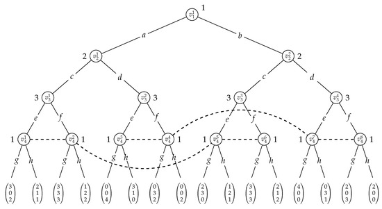
Figure 6. Extensive-form game of imperfect information representing the partial order game in Figure 3 assuming topological order $(v_1,v_2,v_3,v_4)$. Here, for instance, $v_1^1=\left(\right)$, $v_3^2=ad$, and $v_4^4=adf$. The dashed lines connecting vertices indicate the information sets.

The extensive-form game of imperfect information representing the partial order game is then defined for the same set N of players. We define the game tree $(V^{\prime },E^{\prime })$ such that $V^{\prime }$ is the set of all prefixes of terminal histories in $A_{v_1}\times \cdots \times A_{v_{\left|V\right|}}$, with $\left(\right)$ being the root node. The player active at each history/vertex ${\mathbf{h}}_{v_k}=(a_{v_1},\cdots ,a_{v_k})$ in $V^{\prime }$, we identify with the player that is active at $v_{k+1}$ in the partial order game. At each of these vertices/histories this player has $A_{v_{k+1}}$ as the set of actions to chose from. In particular, $i_{v_1}$ is the player active at $\left(\right)$ and has $A_{v_1}$ as action set. Accordingly, all prefixes/histories of the same length are assigned to the same player and each of them have the same action set. For $v,w\in V^{\prime }$, we then have $v{E}^{\prime }w$ if and only if $w=va$ for some $a\in A_v$, as expected.

Every leaf/terminal history $\mathbf{h}=(a_{v_1},\cdots ,a_{v_{\left|V\right|}})$ and player i we associate with the utility value $u_i^{\mathbf{h}}=(a_{v_1},\cdots ,a_{v_{\left|V\right|}})$, where $u_i$ denotes player i’s utility function in the partial order game. Note that in our construction, every terminal history corresponds with a full action profile.

The definition of the information sets is crucial. For every internal vertex/history $\mathbf{h}=(a_{v_1},\cdots ,a_{v_k})$, we formally define these such that

$$\left[(a_{v_1},\cdots ,a_{v_k})\right]=\{(a_{v_1}^{\prime },\cdots ,a_{v_k}^{\prime }):a_y^{\prime }=a_y\mathrm{for}\mathrm{all}\mathrm{parents}y\mathrm{of}{v}_{k+1}\}.$$

Intuitively, a player can only distinguish a vertex/history $\mathbf{h}=(a_{v_1},\cdots ,a_{v_k})$ where it is active from those vertices/histories of the same length that differ on the choice of action in at least one if its parents in the partial order game. All other vertices/histories of the same length belong to the same information set. For an example, consider Figure 6, where vertices $v_4^2=acf$ and $v_4^5=bce$ are in the same information set for player 1. This is because, in the underlying partial order game (depicted in Figure 3), vertex $v_2$ is the only parent of $v_4$ and the histories $acf$ and $bce$ both specify action c for $v_2$. Finally, we define the set of player i’s information sets as

$${\mathcal{I}}_i=\{\left[v^{\prime }\right]:v^{\prime }\in V^{\prime }\mathrm{and}i\mathrm{is}\mathrm{active}\mathrm{at}{v}^{\prime }\}.$$

To see that the extensive-form game defined through this transformation is strategically equivalent to the original partial order game, first consider an arbitrary vertex $v_j$ along with its parents Y in the partial order game. Together with $v_j$ itself, each profile ${\mathbf{a}}_Y$ in ${\mathbf{A}}_Y$ defines a unique information set for i defined as

$$I\left(v_j,{\mathbf{a}}_Y\right)=\{{\mathbf{a}}^{\prime }\in A_{v_1}\times \cdots \times A_{v_{j-1}}:{\mathbf{a}}_Y={\mathbf{a}}_Y^{\prime }\}.$$

Let $\theta$ be the function that maps each pair $(v_j,{\mathbf{a}}_Y)$ to information set $I(v_j,{\mathbf{a}}_Y)$.

Observe that defined thus, $\theta$ is both injective and surjective. We now find that we can extend $\theta$ to a function $\widehat{\theta }$ that maps each conditional strategy ${\mathbf{f}}_i=(f_{v_{i_1}},\cdots ,f_{v_{i_k}})$ in the partial order game to a strategy ${\widehat{\mathbf{f}}}_i:{\mathcal{I}}_i\to A_i$ for player i in the extensive-form game. To do so, define ${\widehat{\mathbf{f}}}_i$ such that for each each information set $I\in {\mathcal{I}}_i$ with ${\theta }^{-1}\left(I\right)=(v_j,{\mathbf{a}}_Y)$

$${\widehat{\mathbf{f}}}_i\left(I\right)=f_{v_j}\left({\mathbf{a}}_Y\right).$$

Observe that the extended function $\widehat{\theta }$ is also bijective. Moreover, some reflection reveals that the full action profile ${\mathbf{a}}^{\mathbf{f}}=(a_{v_1}^{\mathbf{f}},\cdots ,a_{v_{\left|V\right|}}^{\mathbf{f}})$ determined by conditional strategy profile $\mathbf{f}=({\mathbf{f}}_1,\cdots ,{\mathbf{f}}_{\left|N\right|})$ in the partial order game will be identical to the one determined by the strategy profile $\widehat{\mathbf{f}}=({\widehat{\mathbf{f}}}_1,\cdots ,{\widehat{\mathbf{f}}}_{\left|N\right|})$ in the extensive-form game. Having defined the players’ utilities in the extensive-form game as we did, we may conclude that the partial order game is strategically equivalent to the extensive game of imperfect information. Formally:

Proposition 1.

A partial order game and the extensive-form game obtained from it on basis of a given topological sorting, as described in this section, are strategically equivalent.

This result means that, with respect to game theoretic analysis, partial order games are in a precise technical sense (i.e., with respect to strategic equivalence), no more expressive than extensive form games: any scenario we can model with a partial order game can also be modelled with an extensive form game. However, this does not mean that partial order games are redundant. The translation from partial order game to extensive form game comes at the expense of a blow-up in the size of the game: if $|A_v|\ge 2$ for every vertex v, then $V^{\prime }=\mathsf{\Omega }(2^{\left|V\right|})$. The practical upshot of this is that there are situations that we can capture using the partial order model that would be infeasible to capture with the extensive form. In addition, we argue that the partial order representation can in some cases be much more comprehensible than the extensive form: compare the partial order game in Figure 3 with its extensive form representation in Figure 6. Understanding what is going on (and in particular, the informational dependencies present) in the latter representation requires much more work than in the former.

Note that, for total-order games, the construction yields (finite) extensive-form games of perfect information (see Figure 7 and Figure 8 below). This can easily be appreciated by recalling that a total order game allows for only one topological order, say $(v_1,\cdots ,v_{V_{\left|V\right|}})$. Thus, for every $1\le j\le \left|V\right|$ we have that the parents of $v_j$ are all vertices in $Y=\{v_1,\cdots ,v_{j-1}\}$. However, then, obviously, $I\left(v_j,{\mathbf{a}}_Y\right)=\{{\mathbf{a}}^{\prime }\in A_{v_1}\times \cdots \times A_{v_{j-1}}:{\mathbf{a}}_Y={\mathbf{a}}_Y^{\prime }\}$ will be a singleton for every action profile ${\mathbf{a}}_Y$, and the resulting game one of perfect information. As finite extensive-form games of perfect information can be solved by backwards induction (cf. e.g., in [4], Chapter 7), it follows as a corollary that total-order games always admit Nash equilibria in general.

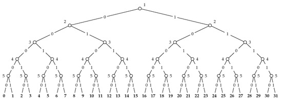
Figure 7. Extensive-form game of perfect information illustrating Proposition 4. for every $0\le n\le 31$, we have $\mathbf{n}$ denote the vector ${(n,n,n,n,n)}^T$.

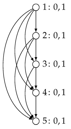
Figure 8. The DAG for the partial order game with five players illustrating Proposition 4.

Proposition 2.

Total-order games always have at least one Nash equilibrium.

We conclude this section with a remark about topological sortings. The DAG of a partial order game may not have a unique topological sorting over its nodes and, under the transformation described above, different topological sortings may lead to different extensive-form games. This is illustrated by Figure 6 and Figure 9, which both depict extensive-form games obtained from the partial order game in our first example in Figure 3. These extensive-form games we obtain using our transformation for the topological sortings $(v_1,v_2,v_3,v_4)$ and $(v_1,v_2,v_4,v_3)$, respectively, and are clearly distinct. Yet, they are strategically equivalent. A formal proof that any two extensive-form games that are obtained using our transformations for different topological orders will be strategically equivalent is beyond the scope of this paper. It suffices to say that it is due to the so-called Interchange of Moves principle, which is one of the four Thompson transformations [26] and informally captures the idea that in extensive-form games of imperfect information “the order of play is immaterial if one player does not have any information about the other player’s action when making his choice” (see in [5], page 224).

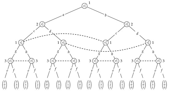
Figure 9. Extensive-form game of imperfect information representing the partial order game in Figure 5 assuming topological ordering $(v_1,v_2,v_4,v_3)$. The dashed lines connecting vertices indicate the information sets.

4.4.2. Partial Order Games as a Concise Representation of Extensive-Form Games

As we noted above, the transformation of partial order games to extensive-form games presented in the previous section may give rise to an exponential blow-up. Reasoning conversely, this raises the claim that partial order games could be seen as providing a concise representation of extensive form games. In this section, we argue that if the utilities in partial order games are represented by Boolean circuits, then this claim is supported.

In Section 2.3, we recalled the well-known fact that transforming an extensive-form game to a normal-form game leads to an exponential blow-up. One reason for this is that, in extensive-form games, a player’s utilities are represented by an association of utility values to leaf nodes/terminal histories. One leaf node, however, may be reached by playing different strategy profiles, or even different action profiles, whereas in normal-form games utilities are specified for each strategy/action profile separately.

In partial order games, the players’ utilities are also modelled as an association of action profiles (not strategy profiles) and utility values. We find, however, that an exponential blow-up can be avoided when the players’ utility functions are represented by Boolean circuits.

The main idea behind this can be explained by means of an example. Consider again the extensive form in Figure 1, where each action has already been labelled with its local index in binary. For each internal vertex/non-terminal history v with action set $A_v$, we introduce $\lceil {log}_2\left|A_v\right|\rceil$ Boolean variables $x_1^v,\cdots ,x_{\lceil {log}_2\left|A_v\right|\rceil }^v$. In the example, we introduced variables x for $v_0$, y and $y^{\prime }$ for $v_1$, z for $v_2$, and $x^{\prime }$ for $v_3$. A truth-value assignment $\alpha$ to these variables for all vertices then defines an action profile ${\mathbf{a}}^{\alpha }=(a_{v_1}^{\alpha },\cdots ,a_{v_{\left|V\right|}}^{\alpha })$ such that $a_j^{\alpha }$ is the action in $A_v$ with numerical index $\mathit{num}(\alpha \left(x_1\right),\cdots ,\alpha \left(x_{\lceil {log}_2\left|A_v\right|\rceil }\right))$, for each vertex v. In our example, for instance, the assignment ${\alpha }^{*}$ that sets x and $y^{\prime }$ to false and y, z, and $x^{\prime }$ to true, corresponds to the action profile $(a_0,b_{10},c_1,d_1)$. With all utilities in our example being either 0 or 1, we can now associate a Boolean formula ${\phi }_{u_i}$ that characterises each player’s utility function, in the sense that assignment $\alpha$ satisfies ${\phi }_{u_i}$ if and only if $u_i\left({\mathbf{a}}^{\alpha }\right)=1$. In our example, such a formula ${\phi }_{u_1}$ representing player 1’s binary utility function could then for instance be obtained by first defining recursively a formula ${\phi }_v$ for each vertex v as follows. First, for each leaf node/terminal history $\mathbf{h}$, we set ${\phi }_{\mathbf{h}}$ = $\top$, if $u_i^{\mathbf{h}}$ = 1, and ${\phi }_{\mathbf{h}}$ = $\perp$, if ui=0$u_i^{\mathbf{h}}$ = 0. In our example, we thus have, for instance, ${\phi }_{a_0{b}_{01}}=\perp$ and ${\phi }_{a_1{c}_1{d}_1}=\top$. For every internal vertex/non-terminal history v, furthermore, we then set

$${\phi }_v={\bigvee }_{a\in A_v}({\chi }_a\wedge {\phi }_{va}),$$

where ${\chi }_a={\tilde{x}}_1^v\wedge \dots \wedge {\tilde{x}}_{\lceil {log}_2\left|A_v\right|\rceil }^c$ characterises the local index k of a, that is ${\tilde{x}}_j^v=x_j^v$, if $b_j=1$, and ${\tilde{x}}_j^v=\neg {\tilde{x}}_j^c$ if $b_j=0$, where $\mathit{bin}\left(k\right)=b_1\dots b_{\lceil {log}_2\left|A_v\right|\rceil }$. Then, set ${\phi }_i={\phi }_{\left(\right)}$. Thus, in our example we get, subsequently,

$$\begin{array}{cc}\hfill {\phi }_{v_3}& =({\overline{x}}^{\prime }\wedge \perp )\vee (x^{\prime }\wedge \top )\hfill \\ \hfill {\phi }_{v_2}& =(\overline{z}\wedge \perp )\vee (z\wedge {\phi }_{v_3})\hfill \\ \hfill {\phi }_{v_1}& =(\overline{y}{\overline{y}}^{\prime }\wedge \top )\vee (\overline{y}{y}^{\prime }\wedge \perp )\vee (y{\overline{y}}^{\prime }\wedge \top )\vee (y{y}^{\prime }\wedge \perp )\hfill \\ \hfill {\phi }_{v_0}& =(\overline{x}\wedge {\phi }_{v_1})\vee (x\wedge {\phi }_{v_2})\hfill \end{array}$$

Finally, we obtain ${\phi }_{u_1}={\phi }_{v_0}$. in our example, we now find, for instance, that assignment ${\alpha }^{*}$ does not satisfy ${\phi }_{u_i}$ and that $u_i\left({\mathbf{a}}^{{\alpha }^{*}}\right)=0$.

This procedure is general and can be applied to every extensive-form game. The crucial thing to observe is that each variable x occurs at most $2^{\lceil {log}_2\left|A_v\right|\rceil }=O\left(\right|A_v\left|\right)$ times in ${\phi }_{u_i}$. Therefore, the size of ${\phi }_{u_i}$ is still polynomial in the size of game and, thus, there is a polynomial-sized Boolean circuit ${\mathbb{C}}_{u_i}$ representing the Boolean function ${\beta }_{{\phi }_{u_i}}$. Finally, any rational-valued utility function $u_i:A_{v_1}\times \cdots \times A_{v_{\left|V\right|}}\to \mathbb{Q}$ can be represented by a linear combination of such circuits, and we may conclude that $u_i$ can be represented by a Boolean circuit whose size is polynomial in the size of the extensive-form game, giving us the following lemma.

Lemma 3.

Let $u_i:S_1\times \cdots \times S_{\left|N\right|}\to \mathbb{Q}$ be the utility function of a player i in an extensive-form game. Then, $u_i$ can be represented by a Boolean circuit that is of a size polynomial in the size of the extensive-form game.

Recall that an extensive-form game and a partial order game are said to be strategically equivalent if they give rise to strategically equivalent normal-form games. We now find that, provided that utilities may be represented by Boolean circuits, every extensive-form game can be represented by a strategically equivalent partial order game without giving rise to more than an at most a polynomial blowup.

Proposition 3.

For every extensive-form game, there is a strategically equivalent partial order game whose size is at most polynomially larger than that of the extensive-form game.

Sketch of Proof.

Let an extensive form for players in a set N be based on a tree $(V,E)$. Let $\mathcal{I}$ be the information sets of this game. We construct a partial order game on the trivial DAG $(\mathcal{I},Ø)$, which is obviously polynomial in the size of the extensive-form game. We associate with each information set I in $\mathcal{I}$ the same player and the same action set $A_I$ as in the extensive-form game. For every player i with ${\mathcal{I}}_i=\{I_1,\cdots ,I_k\}$, we can define a bijection that maps every strategy $s_i:{\mathcal{I}}_i\to A_i$ for i in the extensive-form game to a strategy ${\widehat{\mathbf{f}}}_i=({\widehat{f}}_{I_1},\cdots ,{\widehat{f}}_{I_k})$ for player i in the partial order game such that ${\widehat{f}}_{I_j}$ is the strategy that maps the empty sequence $\left(\right)$ to action $s_i\left(I_j\right)$. By virtue of Lemma 3 we may assume the utility function of each player in the extensive-form game can be represented by a polynomially sized Boolean circuit. Accordingly, the the size of the whole partial order game constructed thus is polynomial in the size of the extensive-form game. Conclude by observing that the extensive-form game and the partial order game induce strategically equivalent normal-form games, as desired. □

Proposition 3 shows that every extensive-form game of perfect-information can be represented by a partial order game at the cost of an at most polynomial blow-up. In some cases, moreover, we find that partial order games may be exponentially smaller than any extensive-form game of perfect information that is strategically equivalent. Consider the following extensive-form game with n players, ordered from 1 to n. Every player has two actions, 0 and 1, at their disposal, but can make their choice dependent on the players that occur before them in the ordering. Each strategy profile $\mathbf{s}$ gives rise to a unique terminal history ${\mathbf{h}}^{\mathbf{s}}=(b_1,\cdots ,b_n)$ of actions in $\{0,1\}$, where each player i plays $b_i$. Accordingly, there are exactly ${\left|\{0,1\}\right|}^n=2^n$ terminal histories or leaves in this extensive-form game. Let the preferences for each player i at each of these terminal histories $\mathbf{h}=(b_1,\cdots ,b_n)$ be given by the utility function such that $u_i^{\mathbf{h}}=\mathit{num}(b_1,\cdots ,b_n)$, where $\mathit{num}(b_1,\cdots ,b_n)$ is the numerical value of the sequence $b_1,\cdots ,b_n)$ conceived as an integer in binary. For instance, $\mathit{num}\left(01101\right)=13$. Then, for each player, every terminal history or leaf yields a unique utility value. See Figure 7 for an illustration of this game for n = 5. To represent this game, an extensive-form game needs to have at least 2ⁿ leaf nodes to account for all the different payoffs a player may get, and thus is of size at least exponential in the number of players.

By contrast, one can represent this game as a partial order game on a transitive graph $(V,E)$, where $V=\{v_1,\dots ,v_n\}$ and $v_{i}E{v}_j$ if and only if i < j. Let player i be assigned to vertex v_i and $A_{v_i}=\{0,1\}$ for all $1\le i\le n$. For each player i, the utility function $u_i(b_1,\cdots ,b_n)=\mathit{num}(b_1,\cdots ,b_n)$ can clearly be represented by a Boolean circuit with V input variables, and as many output variables, with the mth input gate immediately leading to the mth output gate with no intermediate logic gates. See Figure 8 for an illustration of the partial order game representing the extensive-form game in Figure 7. Therefore, we have the following result establishing that partial order games can be seen as presenting a concise representation of extensive-form games. Moreover, this observation still holds if attention is restricted to games of perfect information.

Proposition 4.

There exist partial order games for which every strategically equivalent representation as an extensive-form game of imperfect information is at least exponentially as large.

5. Nash Equilibria

We saw in Section 2.2 how every partial order game defines a normal-form game. Accordingly, partial order games are amenable to game-theoretic analysis using the standard non-cooperative solution concepts that are available for normal-form games. In this section, we consider several complexity problems surrounding Nash equilibrium in partial order games.

We have the following lemma that will be useful for proving the complexity results in this section. It states that, if a player has a profitable deviation to a conditional strategy, then they also have a profitable deviation to an unconditional strategy. In other words, if a player has a best response, then they also have an unconditional best response (This is reminiscent of mixed strategies for (finite) normal-form games, where, due to the linearity of expected utility, a player having a best response implies their having a pure best response).

Lemma 4.

Let $\mathbf{f}=({\mathbf{f}}_1,\cdots ,{\mathbf{f}}_n)$ be a profile of conditional strategies. Then, if there is some strategy $g_i$ for player i with $u_i({\mathbf{f}}_{-i},{\mathbf{g}}_i)>u_i\left(\mathbf{f}\right)$, there also is an unconditional strategy ${\mathbf{g}}_i^{\prime }$ such that $u_i({\mathbf{f}}_{-i},{\mathbf{g}}_i^{\prime })>u_i\left(f\right)$. Therefore, $\mathbf{f}=(f_{v_1},\cdots ,f_{v_{\left|V\right|}})$ is a Nash equilibrium if and only if $u_i\left(\mathbf{f}\right)\ge u_i({\mathbf{f}}_{-i},{\mathbf{g}}_i^{\prime })$ for all players i and unconditional strategies ${\mathbf{g}}^{\prime }$ for i.

Proof. 

Assume that there is some strategy $g_i$ for player i with $u_i({\mathbf{f}}_{-i},{\mathbf{g}}_i)>u_i\left(\mathbf{f}\right)$. Let $v_{i_1},\cdots ,v_{i_k}$ be the vertices assigned to player i. Moreover, let ${\mathbf{a}}^{({\mathbf{f}}_{-i},{\mathbf{g}}_i)}=(a_{v_1}^{*},\cdots ,a_{v_{\left|V\right|}}^{*})$. Now define ${\mathbf{g}}_i^{\prime }=(g_{v_{i_1}}^{\prime },\cdots ,g_{v_{i_k}}^{\prime })$ such that for every $1\le j\le k$, and every profile $(a_{u_1},\cdots ,a_{u_{\ell }})$, where $u_1,\cdots ,u_{\ell }$ are the parents of $v_{i_j}$,

$$g_{v_{i_j}}^{\prime }(a_{u_1},\cdots ,a_{u_{\ell }})=g_{v_{i_j}}(a_{u_1}^{*},\cdots ,a_{u_{\ell }}^{*}).$$

Thus, ${\mathbf{g}}_i^{\prime }$ is clearly an unconditional strategy for player i. Let ${\mathbf{a}}^{({\mathbf{f}}_{-i},{\mathbf{g}}_i^{\prime })}=(a_{v_1}^{**},\cdots ,a_{v_{\left|V\right|}}^{**})$. By a straightforward induction on $\mathit{depth}\left(w\right)$ it can then easily be shown that $a_w^{**}=a_w^{*}$ for every vertex w. And thus, $u_i({\mathbf{f}}_{-i},{\mathbf{g}}_i^{\prime })>u_i\left(\mathbf{f}\right)$, giving us the result. □

The key point about this lemma is that unconditional strategies are small, in the sense that unconditional strategies can be represented by Boolean circuits whose size is polynomial in the set of actions (see Section 3.1, above). Thus, when we are considering whether a player has a beneficial deviation, we can without loss of generality restrict our attention to small strategies. This has implications for the complexity of the decision problems we consider.

The dependency graph provides a concise representation of the sets of conditional strategies available to the players. A single strategy $f_v$ for the player i playing at vertex v, however, has to take into account all profiles $(a_{y_1},\cdots ,a_{y_k})$ in $A_{y_1}\times \cdots \times A_{y_k}$, where $y_1,\cdots ,y_k$ are the parents of v. The number of these profiles tends to be exponential in k, the number of parents, as in all non-trivial cases generally $|A_v|\ge 2$. Similarly, a naive representation of the player’s utilities for the different action profiles tends to be exponential in the number of actions available to the players in the game. However, as the utilities of players are represented by Boolean circuits, there is a straightforward polynomial transformation of Boolean games and Boolean partial order games to general partial order games. This enables us to leverage hardness results for Boolean and partial order Boolean games to obtain hardness results for general partial order games.

We first consider the decision problem of determining whether a given strategy profile is a Nash equilibrium for a given partial order game. Here, we assume that the utility function $u_i$ of each player is represented by a Boolean circuit ${\mathbb{C}}_{u_i}$ and the strategy profile $\mathbf{f}=(f_{v_1},\cdots ,f_{v_{\left|V\right|}})$ is represented by a sequence of $\left|V\right|$ Boolean circuits ${\mathbb{C}}_{f_{v_1}},\cdots ,{\mathbb{C}}_{f_{v_{\left|V\right|}}}$.

is-nash
Given:	Partial order game G and strategy profile $\mathbf{f}=(f_{v_1},\cdots ,f_{v_{\left|V\right|}})$
Problem:	Is $\mathbf{f}$ a Nash equilibrium of G?

We find that is-nash is intractable for partial order games.

Theorem 1.

is-nashis $\mathrm{coNP}$-complete. The problem remains $\mathrm{coNP}$-hard for empty-order games and total-order games.

Proof. 

For membership in $\mathrm{coNP}$, let partial order game G and conditional strategy profile $\mathbf{f}=(f_{v_1},\cdots ,f_{v_{\left|V\right|}})$ be given. We can guess a player i and a strategy ${\mathbf{g}}_i=(g_{v_1},\cdots ,g_{v_m})$, where $v_1,\cdots ,v_m$ are the vertices assigned to i. By virtue of Lemma 4, we may assume that strategies $g_{v_1},\cdots ,g_{v_m}$ are all unconditional strategies. As we saw in Section 3.1, the Boolean circuits ${\mathbb{C}}_{g_{v_1}},\cdots ,{\mathbb{C}}_{g_{v_m}}$ can therefore each be assumed to be of size polynomial in $\left|A\right|$. Now, Lemma 2 allows us to find in polynomial time the utilities $u_i\left({\mathbf{f}}_{-i},{\mathbf{g}}_i\right)$ and $u_i({\mathbf{f}}_{-i},{\mathbf{f}}_i)$. Then, $\mathbf{f}=(f_{v_1},\cdots ,f_{v_{\left|V\right|}})$ is not a Nash equilibrium if and only if $u_i\left({\mathbf{f}}_{-i},{\mathbf{g}}_i\right)>u_i({\mathbf{f}}_{-i},{\mathbf{f}}_i)$, and so we may conclude that is-nash is in $\mathrm{coNP}$.

For $\mathrm{coNP}$-hardness, we reduce from is-nash for Boolean partial order games, which is known to be $\mathrm{coNP}$-hard (see in [1], Proposition 1). Thus, let an instance of is-nash for Boolean partial order games be given by a Boolean game $(N,\mathsf{\Phi },{\mathsf{\Phi }}_1,\cdots ,{\mathsf{\Phi }}_{\left|N\right|},{\gamma }_1,\cdots ,{\gamma }_{\left|N\right|})$, a dependency graph $(\mathsf{\Phi },E)$, and a strategy profile $\mathbf{f}=({\mathbf{f}}_1,\cdots ,{\mathbf{f}}_{\left|N\right|})$, where for each player i strategy ${\mathbf{f}}_i$ is given by a sequence of choice equations $p_1:{\phi }_1$ through $p_m:{\phi }_m$, where ${\mathsf{\Phi }}_i=\{p_1,\cdots ,p_m\}$. In Section 4.1, we argued how this Boolean partial order game coincides with a partial order game with a slightly different representation of strategies and utilities. A similar remark concerns the strategy profile $\mathbf{f}=({\mathbf{f}}_1,\cdots ,{\mathbf{f}}_{\left|N\right|})$. As we found that the transformation of the representation of the game as a Boolean partial order game to the representation of the same game as a partial order game can be effected in polynomial time, we obtain our result. Moreover, because Boolean games are a special type of empty-order games, the problem remains hard for empty-order games as well.

To see that is nash also remains $\mathrm{coNP}$-hard for total-order games, we adapt the proof for the is nash problem for Boolean games as presented in (Wooldridge et al. [15], Proposition 1). We reduce from the complement of satisfiability, the problem of determining if a given Boolean formula $\phi$ is satisfiable. To this end, let $\phi$ a Boolean formula over propositional variables $p_1,\cdots ,p_m$. We construct a total-order Boolean game with one player i controlling $p_1,\cdots ,p_m$ along with an additional variable $p_0$. The dependency graph $(V,E)$ is then given by $V=\{v_{p_0},\cdots ,v_{p_m}\}$ with relation E such that $p_{j}E{p}_k$ if and only if $j<k$. Player i has as goal ${\gamma }_i=\phi \wedge p_0$. Now, consider the strategy profile ${\mathbf{f}}^0=(f_{v_{p_0}}^0,f_{v_{p_1}}^0,\cdots ,f_{v_{p_m}}^0)$ that sets all variables to false, that is, ${\mathbf{f}}^0$ is given by choice equations $p_j:\perp$ for all $0\le j\le m$. Now observe that, as we are dealing with a one-player game, there is a natural surjection that maps each of player i’s strategies $\mathbf{f}$ to valuation ${\alpha }_{{\mathbf{a}}^{\mathbf{f}}}:\{p_0,\cdots ,p_m\}\to \{0,1\}$. It can then easily be appreciated that ${\mathbf{f}}^0$ is a Nash equilibrium in the game constructed if and only if $\phi$ is satisfiable, as desired. □

Another canonical problem is more general, in that it asks whether a partial order game has any Nash equilibria at all, as opposed to whether or not a specific strategy profile is a Nash equilibrium.

non-emptiness
Given:	Partial order game G
Problem:	Does G have a Nash equilibrium?

In view of Proposition 2, non-emptiness is vacuous for total-order games, as in this class of games Nash equilibria are guaranteed to exist. The problem is considerably more difficult, namely $\mathrm{NEXPTIME}$-complete, for general partial order games. It also seems a fair conclusion to draw from this contrast that increase in computational complexity arises from the structure of the dependency graph.

Theorem 2.

non-emptinessis $\mathrm{NEXPTIME}$-complete.

Proof. 

A $\mathrm{NEXPTIME}$ algorithm to decide non-emptiness can be designed along the following lines. First, guess a strategy profile $\mathbf{f}=(f_{v_1},\cdots ,f_{v_{\left|V\right|}})$. Given that strategies $f_v$ are given by a Boolean circuit ${\mathbb{C}}_{f_v}$, this can be achieved in time not more than exponential in $\left|A\right|$, the size of the set of actions. Second, to decide whether $\mathbf{f}=(f_{v_1},\cdots ,f_{v_{\left|V\right|}})$ is a Nash equilibrium, by virtue of Lemma 4, it suffices to check, for all players i and all unconditional strategies ${\mathbf{g}}_i=(g_{v_1},\cdots ,g_{v_{|V_i|}})$ for i, that $u_i\left({\mathbf{f}}_{-i},{\mathbf{f}}_i\right)\ge u_i({\mathbf{f}}_{-i},{\mathbf{g}}_i)$. For player i, there are $|A_{v_1}\times \cdots \times A_{v_{|V_i|}}|$ unconditional strategies which is upper bounded by ${\left|A\right|}^{\left|V\right|}$. Moreover, as we have seen in Section 3.1, each of these unconditional strategies can be represented by a sequence of Boolean circuits of size polynomial in $\left|A\right|$. Furthermore, the action profiles ${\mathbf{a}}^{({\mathbf{f}}_{-i},{\mathbf{f}}_i)}$ and ${\mathbf{a}}^{({\mathbf{f}}_{-i},{\mathbf{g}}_i)}$ can be computed in time exponential in $\left|A\right|$, by virtue of Lemma 1 and each circuit involved being at most exponential in the size of $\left|A\right|$. Finally, on the basis of Lemma 2, we can check in time polynomial in $\left|A\right|$ the utilities for player i on action profiles ${\mathbf{a}}^{({\mathbf{f}}_{-i},{\mathbf{f}}_i)}$ and ${\mathbf{a}}^{({\mathbf{f}}_{-i},{\mathbf{g}}_i)}$, and therefore also whether $u_i\left({\mathbf{f}}_{-i},{\mathbf{f}}_i\right)\ge u_i({\mathbf{f}}_{-i},{\mathbf{g}}_i)$. Altogether, the algorithm runs in non-deterministic exponential time.

A proof of $\mathrm{NEXPTIME}$-hardness of non-emptiness can be achieved by a reduction from the non-emptiness problem for Boolean partial order games. We rely here on the same direct reduction as in the proof of Theorem 1, above. $\mathrm{NEXPTIME}$-hardness for Boolean partial order games was established by [1], giving us the result. □

If we restrict attention to empty-order games, however, non-emptiness has considerably lower computational costs, even though the problem still remains ${\mathsf{\Sigma }}_2^p$-hard. Key to this result is the observation that for empty-order games all strategies are unconditional, and, thus, they can be represented by Boolean circuits of polynomial size (see Section 3.1).

Theorem 3.

For empty-order games,non-emptinessis ${\mathsf{\Sigma }}_2^p$-complete.

Proof. 

To see that non-emptiness is in ${\mathsf{\Sigma }}_2^p$, recall that ${\mathsf{\Sigma }}_2^p={\mathrm{NP}}^{\mathrm{coNP}}$, that is, the set of problems that can be solved in polynomial time on a non-deterministic Turing machine with a $\mathrm{coNP}$-oracle. Furthermore, recall that strategy profiles in empty-order games are unconditional and are of the form $f_v:\left\{\left(\right)\right\}\to A_v$. Moreover, they can be represented by Boolean circuits of polynomial size (see Section 3.1, above). Accordingly, given an empty-order game, we can guess an unconditional strategy profile $\mathbf{f}=(f_{v_1},\cdots ,f_{v_{\left|V\right|}})$, and consult the $\mathrm{coNP}$-oracle to check whether $\mathbf{f}$ is a Nash equilibrium. Theorem 1 guarantees that the latter is feasible.

For ${\mathsf{\Sigma }}_2^p$-hardness, recall that Boolean games constitute a subclass of empty-order partial order games. ${\mathsf{\Sigma }}_2^p$-hardness then follows immediately from non-emptiness being ${\mathsf{\Sigma }}_2^p$-hard for Boolean games (see in [13], Proposition 5). □

Recall that in partial order games, strategy profiles and action profiles are essentially different objects. As a natural counterpart to the is nash problem, we therefore now consider the decision problem whether a given action profile is sustained by a Nash equilibrium in a partial order game.

is nash actions
Given:	Partial order game G and action profile $\mathbf{a}=(a_{v_1},\cdots ,a_{v_{\left|V\right|}})$
Problem:	Is $\mathbf{a}$ sustained by a Nash equilibrium?

In sharp contrast to $\mathrm{coNP}$-completeness of is nash, we find that is nash actions is $\mathrm{NEXPTIME}$-complete. From the perspective of computational complexity, is nash actions appears to be more kindred to the non-emptiness problem for partial order games. In this connection, it is worth observing that the proof of Bradfield et al. regarding the $\mathrm{NEXPTIME}$-completeness of non-emptiness for Boolean partial order games in [1] relied on a reduction from dependency quantifier boolean formula game, which is defined as follows.

An instance of dqbfg is a tuple $⟨\phi ,X_1,X_2,Y_1,Y_2⟩$, where $\phi$ is a Boolean formula $\phi$ and $\{X_1,X_2,Y_1,Y_2\}$ a partition of the propositional variables over which $\phi$ is defined. dqbfg then concerns the following game with three players—B (‘Black’), $W_1$ (‘White 1’), and $W_2$ (‘White 2’)—where B forms one team and $W_1$ and $W_2$ another team W. Player B chooses an assignment for the variables in $X_1\cup X_2=\{x_1^1,\cdots ,x_{|X_1|}^1\}\cup \{x_1^2,\cdots ,x_{|X_2|}^2\}$, player $W_1$ for those in $Y_1=\{y_1^1,\cdots ,y_{|Y_1|}^1\}$, and player $W_2$ for those in $Y_2=\{y_1^2,\cdots ,y_{|Y_2|}^2\}$. Player B chooses first, then $W_1$ and $W_2$ choose, on the understanding that $W_1$ can only see the assignment B chooses for $W_1$ and $W_2$ only the assignment B chooses for $Y_2$. Team B aims to make $\phi$ true, whereas team W’s goal is to make $\phi$ false. If the overall assignment for $X_1\cup X_2\cup Y_1\cup Y_2$ satisfies $\phi$, then B wins, otherwise W. A positive instance of dqbfg is when team W has a winning strategy. dependency quantifier boolean formula game was shown to be $\mathrm{NEXPTIME}$-complete by Hearn and Demaine in [27].

Theorem 4.

is nash actionsis $\mathrm{NEXPTIME}$-complete.

Proof. 

For membership in $\mathrm{NEXPTIME}$, let $\mathbf{a}=(a_{v_1},\cdots ,a_{v_{\left|V\right|}})$ be the action profile that is given as input. Recall from the proof of Theorem 2 that we can guess a strategy profile $\mathbf{f}$ and check whether it is a Nash equilibrium in exponential time, provided that $\mathbf{f}$ is represented by a Boolean circuit. By Lemma 1 we know we can additionally compute ${\mathbf{a}}^{\mathbf{f}}$ in polynomial time and check whether ${\mathbf{a}}^{\mathbf{f}}=\mathbf{a}$. As the latter can also be achieved in polynomial time, we obtain our result.

For $\mathrm{NEXPTIME}$-hardness, we reduce from dependency quantifier boolean formula game (dqbfg). Given an instance $⟨\phi ,X_1,X_2,Y_1,Y_2⟩$ of dqbfg we construct a partial order Boolean game with the same three players, with B controlling the variables in $X_1\cup X_2\cup \left\{x_0\right\}$, player $W_1$ those in $Y_1$, and player $W_2$ those in $Y_2$, where $x_0$ is a “fresh” variable not in $X_1\cup X_2\cup Y_1\cup Y_2$. Let the players’ goals be given by

$$\begin{array}{cccc}\hfill {\gamma }_B& =x_0\wedge \phi \hfill & \hfill {\gamma }_{W_1}={\gamma }_{W_2}& =\perp \hfill \end{array}$$

The dependency graph $(X_1\cup X_2\cup Y_1\cup Y_2\cup \left\{x_0\right\},E)$ is defined such that

(i)

$x_1 E y_1$, for all $x_1\in X_1$ and $y_1\in Y_1$,

(ii)

$x_2 E y_2$, for all $x_2\in X_2$ and $y_2\in Y_2$,

(iii)

$x_0 E z,$ for all $z\in X_1\cup X_2\cup Y_1\cup Y_2$.

Now, consider the action profile

$$\overline{\mathbf{a}}=({\overline{x}}_0,{\overline{x}}_1^1,\cdots {\overline{x}}_{|X_1|}^1,{\overline{x}}_1^2\cdots ,{\overline{x}}_{|X_2|}^2,{\overline{y}}_1^2,\cdots {\overline{y}}_{|Y_1|}^1,{\overline{y}}_1^2\cdots ,{\overline{y}}_{|Y_2|}^2),$$

which sets all variables, including $x_0$, to false. Note that none of the three players win if $\overline{\mathbf{a}}$ is played. We are now in a position to prove that $⟨\phi ,X_1,X_2,Y_1,Y_2⟩$ is a positive instance of dqbfg if and only if $\overline{\mathbf{a}}$ is sustained by a Nash equilibrium in the partial order Boolean game constructed.

First assume that $⟨\phi ,X_1,X_2,Y_1,Y_2⟩$ is positive instance of dqbfg. Then, the white team has a joint winning strategy in the original dqbfg-game given by Boolean functions ${\beta }_1$ and ${\beta }_2$ on the variables $X_1$ and $X_2$, respectively. Then, define strategies ${\mathbf{f}}_{W_1}^{*}$ and ${\mathbf{f}}_{W_2}^{*}$ for $W_1$ and $W_2$, respectively, in the Boolean partial order game, that are given by the following choice equations for $i=1,2$ and $j=1,\cdots ,|Y_i|$:

$$y_j^i:(x_0\to {\phi }_{{\beta }_i}(x_1^i,\cdots ,x_{|X_i|}^i))\wedge ({\overline{x}}_0\to \perp )$$

As the dependency graph $(V,E)$ respects the information dependencies of the dqbfg-instance, observe that ${\mathbf{f}}_{W_1}$ and ${\mathbf{f}}_{W_2}$ together embody a winning strategy to render $\phi$ false, if $x_0$ is played. Let B’s unconditional strategy ${\mathbf{f}}_B^{*}$ be defined by the choice equations of the form $x_j^i:\perp$, setting $x_j^i$ to false for all for $i=1,2$ and $j=1,\cdots ,|X_i|$. Observe that, defined thus, ${\mathbf{a}}^{{\mathbf{f}}^{*}}=\overline{\mathbf{a}}$. Also note that ${\mathbf{f}}^{*}=({\mathbf{f}}_B^{*},{\mathbf{f}}_{W_1}^{*},{\mathbf{f}}_{W_2}^{*})$ is a Nash equilibrium. As $x_0$ will be set to false, all players lose when ${\mathbf{f}}^{*}$ is played, but none has an incentive to deviate either. Player B could only hope to win by setting at least $x_0$ to true. If so, however, $W_1$ and $W_2$ are playing a winning strategy against B, dashing all the latter’s hopes to win after all. Players $W_1$ and $W_2$ will lose, no matter which strategy they adopt. As a consequence, they do not want to deviate either, and we may conclude that ${\mathbf{f}}^{*}$ is a Nash equilibrium sustaining action profile $\overline{\mathbf{a}}$.

Finally, assume that $⟨\phi ,X_1,X_2,Y_1,Y_2⟩$ is a negative instance of dqbfg. Then, team W does not have a winning strategy, meaning that for every strategy ${\mathbf{f}}_W=({\mathbf{f}}_{W_1},{\mathbf{f}}_{W_2})$, player B has a best response ${\mathbf{f}}_B^{\prime }$ such that B wins under $\mathbf{f}=({\mathbf{f}}_{W_1},{\mathbf{f}}_{W_2},{\mathbf{f}}_B^{\prime })$. Now, consider the partial order Boolean game and an arbitrary strategy profile $\overline{\mathbf{f}}$ with ${\mathbf{a}}^{\overline{\mathbf{f}}}=\overline{\mathbf{a}}$. Some reflection reveals that under these circumstances, player B has a strategy ${\mathbf{f}}_B^{\prime }$ at their disposal setting $x_0$ to true and incorporating a winning response to ${\overline{\mathbf{f}}}_W=({\overline{\mathbf{f}}}_{W_1},{\overline{\mathbf{f}}}_{W_2})$. Therefore, player B has an incentive to unilaterally deviate from $\overline{\mathbf{f}}$ and play ${\mathbf{f}}_B^{\prime }$ instead. We may conclude that $\overline{\mathbf{f}}$ is not a Nash equilibrium, as desired. □

For the two extremal classes of empty-order games and total order games, is nash actions are less computationally demanding. More precisely, the problem is $\mathrm{coNP}$-complete for empty-order games and $\mathrm{PSPACE}$-complete for total-order games. The proof of the former statement is relatively straightforward, when one realises that in empty-order games all strategies are unconditional and that, consequently, there is a natural bijection between action profiles and strategy profiles.

Theorem 5.

For empty-order games,is nash actionsis $\mathrm{coNP}$-complete.

Proof. 

First recall that, in empty-order games, there is a natural bijection between action profiles and strategy profiles, mapping each action profile $\mathbf{a}=(a_{v_1},\cdots ,a_{v_{\left|V\right|}})$ to strategy profile ${\mathbf{f}}^{\mathbf{a}}=(f_{v_1}^{a_{v_1}},\cdots ,f_{v_{\left|V\right|}}^{a_{v_{\left|V\right|}}})$, where $f_v^{a_v}\left(\left(\right)\right)=a_v$. Thus, all strategy profiles of an empty-order game are of this form. Moreover, for arbitrary action profiles $\mathbf{a}=(a_{v_1},\cdots ,a_{v_{\left|V\right|}})$ and strategy profiles $\mathbf{f}=(f_{v_1},\cdots ,f_{v_{\left|V\right|}})$, we have that

$$\begin{array}{cc}\hfill \mathbf{a}={\mathbf{a}}^{\mathbf{f}}& \mathrm{if}\mathrm{and}\mathrm{only}\mathrm{if}{f}_v^{a_v}=a_v,\mathrm{for}\mathrm{all}v\in V\hfill \\ \hfill & \mathrm{if}\mathrm{and}\mathrm{only}\mathrm{if}\mathbf{f}={\mathbf{f}}^{\mathbf{a}}\hfill \end{array}$$

Moreover, recall that unconditional strategies are represented by polynomial-sized Boolean circuits. Theorem 1 established that is nash is $\mathrm{coNP}$-complete for empty-order games. Altogether, it suffices to show that, for all action profiles $\mathbf{a}=(a_{v_1},\cdots ,a_{v_{\left|V\right|}})$ of a empty-order game,

$$\mathbf{a}\mathrm{is}\mathrm{sustained}\mathrm{by}\mathrm{a}\mathrm{Nash}\mathrm{equilibrium}\mathrm{if}\mathrm{and}\mathrm{only}\mathrm{if}{\mathbf{f}}^{\mathbf{a}}\mathrm{is}\mathrm{a}\mathrm{Nash}\mathrm{equilibrium}.$$

The “if”-direction is immediate. If ${\mathbf{f}}^{\mathbf{a}}$ is a Nash equilibrium, then, by observing that ${\mathbf{a}}^{{\mathbf{f}}^{\mathbf{a}}}=\mathbf{a}$, action profile $\mathbf{a}$ is sustained by some Nash equilibrium, namely ${\mathbf{f}}^{\mathbf{a}}$. For the “only if”-direction, assume there is some strategy profile ${\mathbf{f}}^{*}$ with $\mathbf{a}={\mathbf{a}}^{{\mathbf{f}}^{*}}$. By our earlier observation we find that ${\mathbf{f}}^{*}={\mathbf{f}}^{\mathbf{a}}$. Hence, ${\mathbf{f}}^{\mathbf{a}}$ is a Nash equilibrium, as desired. □

The proof of $\mathrm{PSPACE}$-completeness of is nash actions for total-order games is considerably more involved, and we defer it to the very end of Section 7.2, where the necessary proof elements are in place. Still, we conclude this section with its statement.

Theorem 6.

For total-order games,is nash actionsis PSPACE-complete.

6. Backwards Induction

Backwards induction is the most fundamental technique for the analysis of extensive form games. The basic backward induction algorithm for extensive form games of perfect information runs in time polynomial in the size of the game tree, and computes Nash equilibrium strategy profiles (which are guaranteed to exist in games of perfect information). It is therefore very natural to ask whether approaches based on backward induction might work for partial order games. However, backward induction is not applicable in extensive form games of imperfect information, and as partial order games correspond to imperfect information games, it follows that the technique is not always applicable. This section introduces a backward induction procedure to find pure Nash equilibria in partial order games. Games in which the procedure is well defined—in the sense that the procedure produces at least one strategy profile—we denote as being fit for backwards induction. We relate this latter concept to an informational notion we refer to as scrutability. For games that are fit for backwards induction, we prove that our backwards induction procedure is guaranteed to produce a Nash equilibrium outcome.

6.1. Backwards Induction

Due to their acyclic nature, it would seem that a natural concept of backward induction procedure can straightforwardly be defined for partial order games. Our aim is thus to define a strategy profile ${\mathbf{f}}^{*}=(f_{v_1}^{*},\cdots ,f_{v_{\left|V\right|}}^{*})$ that is obtained in the following fashion. One starts with a vertex v of maximal depth with set of parents $Y=\{y_1,\cdots ,y_k\}$, and one inspects the possible actions—rather than their strategies—the players active at the parents of v can play. Let ${\mathbf{a}}_Y=(a_{y_1},\cdots ,a_{y_k})$ be any such an action profile, suppose i is the player active at v. Then, the action $a_v^{*}=f_v^{*}(a_{y_1},\cdots ,a_{y_k})$ selected by strategy $f_v^{*}$ from $A_v$ should maximise i’s utility against ${\mathbf{a}}_Y$ and all possible choices of action ${\mathbf{b}}_X$ at the vertices in $X=V\backslash (Y\cup \{v\left\}\right)$, provided any such action $a_v^{*}$ exists. Subsequently, with the strategies for the vertices of greatest depth thus fixed, the strategies in ${\mathbf{f}}^{*}$ should recursively find optimal strategies at vertices of lesser depth in a similar fashion.

In the case of partial order games, it is not strictly necessary to proceed recursively on the depth of the vertices. We can, instead, use any topological sorting $\tau =(v_{{\tau }_1},\cdots ,v_{{\tau }_{\left|V\right|}})$ of the vertices that respects the graph and, starting with the vertex $v_{{\tau }_j}$ with maximal index ${\tau }_j=\left|V\right|$, we iterate through $\tau$ until we reach the vertex with minimal topological index. In this section, we will develop this more general concept of backward induction for partial order games that employs a topological order.

Our backwards induction procedure defines recursively a strategy profile ${\mathbf{f}}^{*}=(f_{v_1}^{*},\cdots ,f_{v_{\left|V\right|}}^{*})$ for each vertex v relative to a topological sorting $\tau =(v_{{\tau }_1},\cdots ,v_{{\tau }_{\left|V\right|}})$, and is formally defined as follows. Let v be a vertex with topological index ${\tau }_j$ and let i be the player to move at v. Let $Y=\{y_1,\cdots ,y_k\}$ be the set of parents of v, $Z=\{z_1,\cdots ,z_m\}$ be the set of vertices with a topological index strictly greater than ${\tau }_j$, and $X=\{x_1,\cdots ,x_{\ell }\}$ be given by $V\backslash (Y\cup Z\cup \{v\left\}\right)$. For every profile ${\mathbf{a}}_Y=(a_{y_1},\cdots ,a_{y_k})$, we define $f_v^{*}(a_{y_1},\cdots ,a_{y_k})$ as an action $a_v^{*}$ in $A_v$ such that, for all profiles ${\mathbf{b}}_X=(b_{x_1},\cdots ,b_{x_{\ell }})$,

$$a_v^{*}\in \underset{a_v\in A_v}{arg\; max}{u}_i({\mathbf{b}}_X,{\mathbf{a}}_Y,a_v,{\mathbf{f}}_Z^{*}),$$

(1)

where the basis of this recursion is provided by the case where $Z=Ø$ (Here we exploit the notation ${\mathbf{b}}_X,{\mathbf{a}}_Y,a_v,{\mathbf{f}}_Z^{*}$ to refer to the action profile that results if after $\tau$-history $({\mathbf{b}}_X,{\mathbf{a}}_Y,a_v$ the strategy profile ${\mathbf{f}}^{*}$ is played over the vertices in Z. Formally, ${\mathbf{b}}_X,{\mathbf{a}}_Y,a_v,{\mathbf{f}}_Z^{*}$ is the action profile ${\mathbf{a}}^{\mathbf{g}}$ for strategy profile $\mathbf{g}=({\mathbf{f}}_X^{{\mathbf{b}}_X},{\mathbf{f}}_Y^{{\mathbf{a}}_Y},f_v^{a_v},{\mathbf{f}}_Z^{*})$, where $({\mathbf{f}}_X^{{\mathbf{b}}_X},{\mathbf{f}}_Y^{{\mathbf{a}}_Y},f_v^{a_v})$ is a profile of unconditional strategies (also see page 9, above)). To illustrate this definition, we have the following example.

Example 4.

Consider the utility function for the game depicted in Figure 10, and fix a topological sorting $(v_1,v_2,v_3,v_4)$. From inspection, it can easily be appreciated that the utility to player 1 is only dependent on their own choices at vertices $v_1$ and $v_4$, and player 2’s at vertex $v_2$. At this moment, we can apply the backwards induction procedure as follows. Inspecting their utility function, we find that player 3 chooses as follows at vertex $v_3$:

$$\begin{array}{cccccccc}\hfill f_{v_3}\left(ac\right)& =f\hfill & \hfill f_{v_3}\left(ad\right)& =e\hfill & \hfill f_{v_3}\left(bc\right)& =f\hfill & \hfill f_{v_3}\left(bd\right)& =f\hfill \end{array}$$

Figure 10. The partial order game from Example 1 with a slightly different utility function.

At vertex $v_4$, player 1, can set their strategy such that $f_{v_4}\left(c\right)=g$ and $f_{v_4}\left(d\right)=h$, because they are indifferent to any choice of actions by the other players. Player 2 can have their strategy at $v_2$ depend on player 1’s choice at $v_1$. If player 1 chooses a at $v_1$, then by playing c at $v_2$, action profile $acfg$ will result and player 2 will obtain utility 3. Whereas, by playing d, action profile $adeh$ will ensue, with a utility of 1 for player 2. Therefore, $f_{v_2}\left(a\right)=c$. A similar reasoning yields that, if player 1 chooses b at $v_1$, by playing c at $v_2$, action profile $(b,c,f,g)$ results with utility 0 for player 2, whereas, by playing d, action profile $(b,d,f,h)$ ensues with utility 2 for player 2. Accordingly, $f_{v_2}\left(b\right)=d$. Finally, by playing a at $v_1$, player 1 obtains utility 3, as action profile $(a,c,f,g)$ would be played. Observe that by playing b at $v_1$, player 1 obtains utility 2, as in that case action profile $(b,d,f,h)$ would result. Accordingly, $f_{v_1}\left(\left(\right)\right)=a$. We thus obtain the strategy profile $\mathbf{f}=(f_{v_1}^1,f_{v_2}^2,f_{v_3}^{12},f_{v_4}^2)$ yielding action profile $(a,c,f,g)$ as the backwards induction solution of this game.

Some reflection reveals that on total-order games the procedure defined thus mimics standard backwards induction on the corresponding extensive-form games of perfect information as described in Section 4.4. It is important to note, however, that, on general partial order games, our backwards induction procedure does not always yield a strategy profile ${\mathbf{f}}^{*}$. This is because the outcome of a partial order game—and therefore also the players’ utilities as well as the possibility of finding a utility maximising action—need not be fully determined by the actions chosen at a given vertex v, at v’s parent vertices, and at the vertices with a larger topological index than v.

The outcome may also depend on the actions chosen at vertices of an equal or lesser depth that are not parents of the respective vertex. If so, it may happen that, at some stage of the procedure and at some vertex, no action can be singled out as an unequivocal optimal choice based on the choices at the parent nodes and those at the vertices with a greater topological index alone. This would cause the procedure to stall. More formally, this happens if for some vertex v, there are two different profiles ${\mathbf{b}}_X=(b_{w_1},\cdots ,b_{w_{\ell }})$ and ${\mathbf{b}}_X^{\prime }=(b_{w_1}^{\prime },\cdots ,b_{w_{\ell }}^{\prime })$ such that ${arg\; max}_{a_v\in A_v}{u}_i({\mathbf{b}}_X,{\mathbf{a}}_Y,a_v,{\mathbf{f}}_Z^{*})$ and ${arg\; max}_{a_v\in A_v}{u}_i({\mathbf{b}}_X^{\prime },{\mathbf{a}}_Y,a_v,{\mathbf{f}}_Z^{*})$ are disjoint. The following example illustrates this point.

Example 5.

Consider again the game of Example 1, depicted in Figure 3. Let us first consider the strategies that player 3 can choose at vertex $v_3$. This player has to specify an action from among e and f, for each of the possible action profiles player 1 and 2 can choose at vertices $v_1$ and $v_2$, respectively, that is, for the action profiles $ac$, $ad$, $bc$, and $bd$. Inspecting player 3’s utilities, player 3 should arguably choose $f_{v_3}\left(ac\right)=f$, as no matter what action player 1 chooses at $v_4$, player 3 is better off playing f than playing e. However, how to choose a value for $f_{v_3}\left(ad\right)$ is not so obvious, as the optimal choice depends on whether player 1 chooses g or h at vertex $v_4$; this is something player 3 may not let their strategy depend upon as not $v_{3}E{v}_4$.

To formalise this issue, we say that a partial order game is fit for backwards induction under a topological sorting $\tau =(v_{{\tau }_1},\cdots ,v_{{\tau }_{\left|V\right|}})$ if, for every vertex v, and every action profile $\mathbf{a}=(a_{v_1},\cdots ,a_{v_{\left|V\right|}})$,

$$\bigcap _{{\mathbf{b}}_X\in {\mathbf{A}}_X}\underset{a_v\in A_v}{arg\; max}{u}_i({\mathbf{b}}_X,{\mathbf{a}}_Y,a_v,{\mathbf{a}}_Z)\ne Ø,$$

where Y is the set of parents of v, Z the set of vertices with a topological index that is not smaller than that of v, and $X=V\backslash (Y\cup Z\cup \{v\left\}\right)$. This ensures that, in Equation (1), the optimal action $a_v^{*}$ is defined for every vertex v. At this point, it is worth observing that for total-order games, the set X will be empty and that they allow for only one topological sorting. It follows that total-order games vacuously satisfy the fit-for-backwards-induction condition under every topological sorting.

We are now in a position to show that our backwards induction procedure always yields a Nash equilibrium in games that are fit for backwards induction.

Theorem 7.

Let G be a partial order game that is fit for backwards induction under a topological order τ. Then, every strategy profile ${\mathbf{f}}^{*}=(f_{v_1}^{*},\cdots ,f_{v_{\left|V\right|}}^{*})$ generated by the backwards induction procedure under τ is a Nash equilibrium.

Proof. 

Let ${\mathbf{f}}^{*}=(f_{v_1}^{*},\cdots ,f_{v_{\left|V\right|}}^{*})$ be a strategy profile that our backwards induction procedure yields for topological order $\tau =(v_{{\tau }_1},\cdots ,v_{{\tau }_{\left|V\right|}})$. Without loss of generality, we may assume that ${\tau }_j=j$ for all $1\le j\le \left|V\right|$, that is, $v_1,\cdots ,v_{\left|V\right|}$ are already topologically ordered. Assume for contradiction that ${\mathbf{f}}^{*}$ is not a Nash equilibrium, that is, there is some strategy ${\mathbf{g}}_i$ for some player i such that $u_i({\mathbf{f}}_{-i}^{*},{\mathbf{g}}_i)>u_i({\mathbf{f}}_{-i}^{*},{\mathbf{f}}_i^{*})$. Let $\mathbf{g}=({\mathbf{f}}_{-i}^{*},{\mathbf{g}}_i)$.

Now, there is at least one vertex $v_j$ with $1\le j\le \left|V\right|$ that is controlled by player i with parents $Y=\{y_1,\cdots ,y_k\}$ for which there is an action profile $\mathbf{x}=(x_{v_1},\cdots ,x_{v_{j-1}})$ in $A_{v_1}\times \cdots \times A_{v_{j-1}}$ such that:

$$u_i(x_{v_1},\cdots ,x_{v_{j-1}},a_{v_j},f_{v_{j+1}}^{*},\cdots ,f_{v_{\left|V\right|}}^{*})<u_i(x_{v_1},\cdots ,x_{v_{j-1}},b_{v_j},g_{v_{j+1}},\cdots ,g_{v_{\left|V\right|}}),$$

(2)

where $a_{v_j}=f_{v_j}^{*}(x_{y_1},\cdots ,x_{y_k})$ and $b_{v_j}=g_{v_j}(x_{y_1},\cdots ,x_{y_k})$ (To see this, let $a^{{\mathbf{f}}^{*}}=(a_{v_1},\cdots ,a_{v_{\left|V\right|}})$ and $a^{\mathbf{g}}=(b_{v_1},\cdots ,b_{v_{\left|V\right|}})$. Then observe that there must be a smallest index $1\le j\le \left|V\right|$ such that $v_j\in V_i$ with $a_{v_j}\ne b_{v_j}$ and $a_{v_m}=b_{v_m}$ for all $1\le m<j$, which provides us with the desired $v_j$). Now we may assume that j is the largest index with $v_j\in V_i$ for which such an action profile, or $\tau$-history, $\mathbf{x}=(x_{v_1},\cdots ,x_{v_{j-1}})$ can be found. Therefore,

$$u_i(x_{v_1},\cdots ,x_{v_{j-1}},b_{v_j},g_{v_{j+1}},\cdots ,g_{v_{\left|V\right|}})\le u_i(x_{v_1},\cdots ,x_{v_{j-1}},b_{v_j},f_{v_{j+1}}^{*},\cdots ,f_{v_{\left|V\right|}}^{*}).$$

(3)

Combining inequalities (2) and (3), we obtain that

$$u_i(x_{v_1},\cdots ,x_{v_{j-1}},a_{v_j},f_{v_{j+1}}^{*},\cdots ,f_{v_{\left|V\right|}}^{*})<u_i(x_{v_1},\cdots ,x_{v_{j-1}},b_{v_j},f_{v_{j+1}}^{*},\cdots ,f_{v_{\left|V\right|}}^{*}).$$

Having assumed $(v_1,\cdots ,v_{\left|V\right|})$ to be ordered topologically, the set $Y=\{y_1,\cdots ,y_k\}$ of parents of $v_j$ is a subset of $\{v_1,\cdots ,v_{j-1}\}$. Let further $X=\{v_1,\cdots ,v_{j-1}\}\backslash Y$ and $Z=\{v_{j+1},\cdots ,v_{\left|V\right|}\}$. Recall that $a_{v_j}=f_{v_j}^{*}(x_{y_1},\cdots ,x_{y_k})$. We then find that, for profile ${\mathbf{x}}_Y$, there is some profile, namely ${\mathbf{x}}_X$, such that

$$f_{v_j}^{*}(x_{y_1},\cdots ,x_{y_k})\notin \underset{a_{v_j}^{\prime }\in A_{v_j}}{arg\; max}{u}_i({\mathbf{x}}_X,{\mathbf{x}}_Y,a_{v_j}^{\prime },{\mathbf{f}}_Z^{*}).$$

It follows that our backwards induction procedure does not provide us with $f_{v_j}^{*}$, which contradicts our initial assumption regarding the profile ${\mathbf{f}}^{*}=(f_{v_1}^{*},\cdots ,f_{v_{\left|V\right|}}^{*})$. □

We also have the following lemma, which is a version of the one-stage-deviation property for partial order games, and which is an almost immediate consequence of the definition of our backwards induction procedure (also see in [28] (pages 108–110) and Osborne and Rubinstein [5] (page 98)). This property will prove to be of great help proving the computational complexity results in Section 7. Intuitively it says that to establish that a strategy profile $\mathbf{f}=(f_{v_1},\cdots ,f_{v_{\left|V\right|}})$ is a backwards induction solution, it suffices to look at deviations by a player from $\mathbf{f}$ at a single vertex $v_k$ given a single history $\mathbf{h}=(a_{v_1},\cdots ,a_{v_k})$. The property is perhaps best understood by considering its contrapositive: strategy profile $\mathbf{f}$ is not a backwards induction solution if there is a single player who has an incentive to deviate from $\mathbf{f}$ at a single vertex $v_k$ given a single history $\mathbf{h}=(a_{v_1},\cdots ,a_{v_k})$. Note that we here assume that the game in question is fit for backwards induction.

Lemma 5 (One-stage-deviation property).

Let the vertices of a partial order game be sorted according to a topological sorting $\tau =(v_1,\cdots ,v_{\left|V\right|})$. Then, for games that are fit for backwards induction, profile $f=(f_{v_1},\cdots ,f_{v_{\left|V\right|}})$ is a backwards induction solution for τ if and only if for every τ-history $(a_{v_1},\cdots ,a_{v_{k-1}})$ with $1\le k\le \left|V\right|$ we have for all $b_{v_k}\in A_{v_k}$:

$$u_i(a_{v_1},\cdots ,a_{v_{k-1}},f_{v_k},f_{v_{k+1}},\cdots ,f_{v_{\left|V\right|}})\ge u_i(a_{v_1},\cdots ,a_{v_{k-1}},b_{v_k},f_{v_{k+1}},\cdots ,f_{v_{\left|V\right|}}),$$

where i is the player assigned to $v_k$.

Proof. 

First assume that $\mathbf{f}=(f_{v_1},\cdots ,f_{v_{\left|V\right|}})$ is a backwards induction solution, and consider an arbitrary $\tau$-history $(a_{v_1},\cdots ,a_{v_{k-1}})$ and equally arbitrary $b_{v_k}$ in $A_{v_k}$. Let Y be the parents of $v_k$ and $X=\{v_1,\cdots ,v_{k-1}\}\backslash Y$. Then,

$$u_i({\mathbf{b}}_X,{\mathbf{a}}_Y,f_{v_k}\left({\mathbf{a}}_Y\right),f_{v_{k+1}},\cdots ,f_{v_{\left|V\right|}})\ge u_i({\mathbf{b}}_X,{\mathbf{a}}_Y,b_{v_k},f_{v_{k+1}},\cdots ,f_{v_{\left|V\right|}}),$$

(4)

for all profiles ${\mathbf{b}}_X$. Now observe that inequality (4) holds for in particular for ${\mathbf{b}}_X={\mathbf{a}}_X$.

For the “if”-direction assume for contraposition that $\mathbf{f}=(f_{v_1},\cdots ,f_{v_{\left|V\right|}})$ is not a backwards induction solution for $\tau$. Then, there is a vertex $v_k$ with minimal topological index, parents Y, and $X=\{v_1,\cdots ,a_{k-1}\}\backslash Y$ such that for some profile ${\mathbf{a}}_Y$, we have for every $a_{v_k}$ in $A_{v_k}$ that there is some profile ${\mathbf{b}}_X$ such that

$$u_i({\mathbf{b}}_X,{\mathbf{a}}_Y,a_{v_k},f_{v_{k+1}},\cdots ,f_{v_{\left|V\right|}})<u_i({\mathbf{b}}_X,{\mathbf{a}}_Y,b_{v_k},f_{v_{k+1}},\cdots ,f_{v_{\left|V\right|}}).$$

(5)

At this point, consider any $a_{v_k}$ in $A_{v_k}$ and let ${\mathbf{b}}_X$ be the accompanying profile for which Equation (5) holds. We can conclude the proof by considering the $\tau$-history $({\mathbf{b}}_X,{\mathbf{a}}_Y)$. □

6.2. Games of Adequate Information

In this section, we propose the class of adequate information games, which are guaranteed to be fit for backwards induction, and, thus, always have a Nash equilibrium. As an auxiliary concept we first introduce the notion of scrutability, an informational criterion specifying on which choices of which players a player can have its decision depend when choosing an action at a specific vertex.

6.2.1. Scrutability

We introduce scrutability as a technical term to reason about the strategic information that is available to the players at each stage of the backwards induction process. Intuitively, let v and w be a vertices at which, respectively, players i and j are active. Then, assuming that the game is fit for backwards induction, a vertex w is scrutable to v if j’s choices of action at w can make a difference as to the optimality of i’s choice of action at v when deciding on a backwards induction strategy at v. Thus, all vertices reachable from v are scrutable, as their backwards induction choices will already have been made. Moreover, the player active at v can have their choice of action depend on the choices of action at the parent nodes of v.

Formally, we say that a vertex w is scrutable to vertex v if either

(i)

w is reachable from v, or

(ii)

$wEv$, that is w is one of v’s parents.

We refer to a vertex that is not scrutable to v as being inscrutable to v. Recall the reachability relation is reflexive, and, thus, vertex v is always scrutable to v itself. Observe that the relations of scrutability and inscrutability are not necessarily symmetric. For instance, if a vertex v is reachable from w, but w is not a parent of v, then v is scrutable to w, but not vice versa. If v is inscrutable to w, and w is also inscrutable to v, we say that v and w are independent.

We differentiate between a vertex being scrutable to a vertex and a vertex being scrutable to a player. For $V_i=\{v_1,\cdots ,v_m\}$ player i’s vertices, we denote by $I_v$ the set of vertices that are inscrutable to v, and by $S_v$ the set of vertices that are scrutable to v. Furthermore, let $I_i=I_{v_1}\cup \cdots \cup I_{v_m}$ and $S_i=V\backslash I_i$ denote the sets of vertices that are inscrutable and scrutable to player i, respectively. That is, if a vertex v is inscrutable to a player i, if v is inscrutable to at least one vertex at which i is active. Vertex v is scrutable to player i, if it is not inscrutable to i, that is, if v is scrutable to all vertices at which i is active. It may be worth observing that in total-order games all vertices will be scrutable from any other vertex.

Furthermore, we introduce a notion of scrutability that is relative to a topological sorting of the vertices. Therefore, let $\tau =(v_{{\tau }_1},\cdots ,v_{{\tau }_{\left|V\right|}})$ be a topological sorting. Then, a vertex w with topological index ${\tau }_w$ is scrutable under $\tau$ to vertex v with topological index ${\tau }_v$, if either

(i)

${\tau }_w\ge {\tau }_v$, or

(ii)

$wEv$, that is w is one of v’s parents.

Any vertex that is not scrutable under $\tau$ is referred to as being inscrutable under $\tau$. For $V_i=\{v_1,\cdots ,v_m\}$ and topological sorting $\tau =(v_{{\tau }_1}\cdots ,v_{{\tau }_{\left|V\right|}})$, we furthermore denote by $I_v^{\tau }$ the set of vertices that are inscrutable to v under $\tau$, and by $S_v^{\tau }$ the set of vertices that are scrutable to v under $\tau$.

Moreover, we define $I_i^{\tau }=I_{v_1}^{\tau }\cup \cdots \cup I_{v_m}^{\tau }$ and $S_i^{\tau }=V\backslash I_i^{\tau }$. Note that the set of vertices scrutable to a player i need not include the set $V_i$ of vertices where i is active.

Given a topological sorting $\tau$ and a vertex v, by Y, we will generally adhere to the following notational conventions. The parents of v we generally denote by Y, the set of vertices inscrutable to v by X, and the set of all vertices that are not parents of v but still scrutable to v by Z. The following example illustrates these concepts.

Example 6.

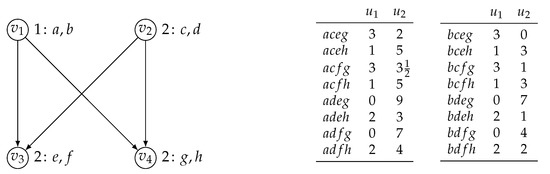
Consider the game depicted in Figure 10. Then, we have the following sets of scrutable and inscrutable vertices.

$$\begin{array}{cccccccc}\hfill S_{v_1}& =\{v_1,v_2,v_3,v_4\}\hfill & \hfill I_{v_1}& =Ø\hfill & \hfill S_1& =\{v_2,v_4\}\hfill & \hfill I_1& =\{v_1,v_3\}\hfill \\ \hfill S_{v_2}& =\{v_1,v_2,v_3,v_4\}\hfill & \hfill I_{v_2}& =Ø\hfill & \hfill S_2& =\{v_1,v_2,v_3,v_4\}\hfill & \hfill I_2& =Ø\hfill \\ \hfill S_{v_3}& =\{v_1,v_2,v_3\}\hfill & \hfill I_{v_3}& =\left\{v_4\right\}\hfill & \hfill S_3& =\{v_1,v_2,v_3\}\hfill & \hfill I_3& =\left\{v_4\right\}\hfill \\ \hfill S_{v_4}& =\{v_2,v_4\}\hfill & \hfill I_{v_4}& =\{v_1,v_3\}\hfill \end{array}$$

For the topological sorting $\tau =(v_1,v_2,v_3,v_4)$, we get

$$\begin{array}{cccccccc}\hfill S_{v_1}^{\tau }& =\{v_1,v_2,v_3,v_4\}\hfill & \hfill I_{v_1}^{\tau }& =Ø\hfill & \hfill S_1^{\tau }& =\{v_2,v_4\}\hfill & \hfill I_1^{\tau }& =\{v_1,v_3\}\hfill \\ \hfill S_{v_2}^{\tau }& =\{v_1,v_2,v_3,v_4\}\hfill & \hfill I_{v_2}^{\tau }& =Ø\hfill & \hfill S_2^{\tau }& =\{v_1,v_2,v_3,v_4\}\hfill & \hfill I_2^{\tau }& =Ø\hfill \\ \hfill S_{v_3}^{\tau }& =\{v_1,v_2,v_3,v_4\}\hfill & \hfill I_{v_3}^{\tau }& =Ø\hfill & \hfill S_3^{\tau }& =\{v_1,v_2,v_3,v_4\}\hfill & \hfill I_3^{\tau }& =Ø\hfill \\ \hfill S_{v_4}^{\tau }& =\{v_2,v_4\}\hfill & \hfill I_{v_4}^{\tau }& =\{v_1,v_3\}\hfill \end{array}$$

By contrast, under topological sorting ${\tau }^{\prime }=(v_1,v_2,v_4,v_3)$, we obtain

$$\begin{array}{cccccccc}\hfill S_{v_1}^{{\tau }^{\prime }}& =\{v_1,v_2,v_3,v_4\}\hfill & \hfill I_{v_1}^{{\tau }^{\prime }}& =Ø\hfill & \hfill S_1^{{\tau }^{\prime }}& =\{v_2,v_3,v_4\}\hfill & \hfill I_1^{{\tau }^{\prime }}& =\left\{v_1\right\}\hfill \\ \hfill S_{v_2}^{{\tau }^{\prime }}& =\{v_1,v_2,v_3,v_4\}\hfill & \hfill I_{v_2}^{{\tau }^{\prime }}& =Ø\hfill & \hfill S_2^{{\tau }^{\prime }}& =\{v_1,v_2,v_3,v_4\}\hfill & \hfill I_2^{{\tau }^{\prime }}& =Ø\hfill \\ \hfill S_{v_3}^{{\tau }^{\prime }}& =\{v_1,v_2,v_3\}\hfill & \hfill I_{v_3}^{{\tau }^{\prime }}& =\left\{v_4\right\}\hfill & \hfill S_3^{{\tau }^{\prime }}& =\{v_1,v_2,v_3\}\hfill & \hfill I_3^{{\tau }^{\prime }}& =\left\{v_4\right\}\hfill \\ \hfill S_{v_4}^{{\tau }^{\prime }}& =\{v_2,v_3,v_4\}\hfill & \hfill I_{v_4}^{{\tau }^{\prime }}& =\left\{v_1\right\}\hfill \end{array}$$

For another example, consider Figure 11 along with topological order $\tau =(v_1,v_2,v_3,v_4)$. We then obtain for the vertices the following sets of scrutable and inscrutable vertices for vertices as well as for players:

$$\begin{array}{cccccccc}\hfill S_{v_1}^{\tau }& =\{v_1,v_2,v_3,v_4\}\hfill & \hfill I_{v_1}^{\tau }& =Ø\hfill & \hfill S_1^{\tau }& =\{v_1,v_2,v_3,v_4\}\hfill & \hfill I_1^{\tau }& =Ø\hfill \\ \hfill S_{v_2}^{\tau }& =\{v_2,v_3,v_4\}\hfill & \hfill I_{v_2}^{\tau }& =\left\{v_1\right\}\hfill & \hfill S_2^{\tau }& =\{v_2,v_4\}\hfill & \hfill I_2^{\tau }& =\{v_1,v_3\}\hfill \\ \hfill S_{v_3}^{\tau }& =\{v_1,v_2,v_3,v_4\}\hfill & \hfill I_{v_3}^{\tau }& =Ø\hfill \\ \hfill S_{v_4}^{\tau }& =\{v_1,v_2,v_4\}\hfill & \hfill I_{v_4}^{\tau }& =\left\{v_3\right\}\hfill \end{array}$$

Figure 11. Another example of a partial order game.

Observe that w being reachable from v implies ${\tau }_w\ge {\tau }_v$, in other words, $S_v\subseteq S_v^{\tau }$ for every topological order $\tau$. Accordingly, plain scrutability is stronger than scrutability under a topological sorting. The following lemma lays down the precise formal interrelationship between scrutability and scrutability under a topological order.

Lemma 6.

Let i be a player of a partial order game and v a vertex controlled by i. Then, for all vertices w,

(i) 

w is scrutable to v if and only if w is scrutable to v under all topological orders τ,

(ii) 

w is inscrutable to v if and only if w is inscrutable to v under some topological order τ,

(iii) 

w is scrutable to i if and only if w is scrutable to i under all topological orders τ,

(iv) 

w is inscrutable to i if and only if w is inscrutable to i under some topological order τ.

Proof. 

We prove part (i) first. Then, parts (ii) through (iv) follow by straightforward set-theoretic reasoning.

(i)

For the “only if”-direction, first assume that w is scrutable to v and consider an arbitrary topological sorting $\tau$ with topological indices ${\tau }_i$ and ${\tau }_j$ for v and w, respectively. Then, either $wEv$ or w is reachable from v, that is, $v{E}^{*}w$. In the former case, we have immediately that w is scrutable to v under $\tau$. In the latter case, observe that then ${\tau }_i<{\tau }_j$ by definition of a topological sorting. It then also follows that w is scrutable to v under $\tau$.

For the “if”-direction, assume for contraposition that w is not scrutable to v. Then, neither $wEv$ nor w being reachable from v hold. In case v is reachable from w, let $\tau$ be any topological order with ${\tau }_i$ and ${\tau }_j$ the topological indices for v and w. Then, ${\tau }_j<{\tau }_i$, and it follows that w is not scrutable under $\tau$. In case v is not reachable from w, let $(V,E)$ be the DAG underlying the partial order game. Then, consider the edge set $E^{\prime }=E\cup \left\{(w,v)\right\}$. The graph $(V,E^{\prime })$ must be acyclic because if $(V,E^{\prime })$ contained a directed cycle, there would be a simple path from v to w not involving the edge $(w,v)$. Therefore, w would also be reachable from v in $(V,E)$, a contradiction. Therefore, $(V,E^{\prime })$ is acyclic and has a topological sorting $\tau$. Observe that $\tau$ is also a topological order for $(V,E)$. Let ${\tau }_i$ and ${\tau }_j$ be the topologic al indices for v and w, respectively. As $w{E}^{\prime }v$, we have ${\tau }_j<{\tau }_i$ and again we may conclude that w is not scrutable to v under $\tau$.

(ii)

This part follows immediately from part (i), by observing the following equivalences:

$$\begin{array}{cc}\hfill & w\mathrm{is}\mathrm{inscrutable}\mathrm{to}v\hfill \\ \hfill & \mathrm{if}\mathrm{and}\mathrm{only}\mathrm{if}w\mathrm{is}\mathrm{not}\mathrm{scrutable}\mathrm{to}v\hfill \\ \hfill & \mathrm{if}\mathrm{and}\mathrm{only}\mathrm{if}w\mathrm{is}\mathrm{not}\mathrm{scrutable}\mathrm{to}v\mathrm{under}\mathrm{some}\mathrm{topological}\mathrm{order}\tau \hfill \\ \hfill & \mathrm{if}\mathrm{and}\mathrm{only}\mathrm{if}w\mathrm{is}\mathrm{inscrutable}\mathrm{to}v\mathrm{under}\mathrm{some}\mathrm{topological}\mathrm{order}\tau \hfill \end{array}$$

(ii)

Let $v_1,\cdots ,v_m$ be the vertices assigned to player i, and let ${\tau }_1,\cdots ,{\tau }_k$ be the topological sortings for the game. From (ii) we obtain that $I_{v_j}=I_{v_j}^{{\tau }_1}\cup \cdots \cup I_{v_j}^{{\tau }_k}$ for every $1\le j\le m$.

(iv)

Therefore,

$$\begin{array}{c}\hfill I_i=\bigcup _{1\le j\le m}{I}_{v_j}=\bigcup _{1\le j\le m}{I}_{v_j}^{{\tau }_1}\cup \cdots \cup I_{v_j}^{{\tau }_k}=\bigcup _{1\le \ell \le k}{I}_{v_1}^{{\tau }_{\ell }}\cup \cdots \cup I_{v_m}^{{\tau }_{\ell }}=\bigcup _{1\le \ell \le k}{I}_i^{{\tau }_{\ell }},\end{array}$$

and it follows that w is inscrutable to i if and only if w is inscrutable to i under some topological sorting. Part (iii) then is an immediate consequence of de Morgan’s law:

$${\displaystyle S_i=V\backslash I_i=V\backslash (I_i^{{\tau }_1}\cup \cdots \cup I_i^{{\tau }_k})=V\backslash I_i^{{\tau }_1}\cap \cdots \cap V\backslash I_i^{{\tau }_k}=S_{v_1}^{{\tau }_1}\cap \cdots \cap S_i^{{\tau }_k}=\bigcap _{1\le \ell \le k}{S}_i^{{\tau }_{\ell }}.}$$

Therefore, w is scrutable to i if and only if i is scrutable to i under all topological sortings.

This concludes the proof. □

6.2.2. Games of Adequate Information

In this section, we define a class of partial order games, which we refer to as games of adequate information. We prove that games of adequate information are fit for backward induction, and thus, on account of Theorem 7, allow for Nash equilibria. For this, we require that each player at each vertex assigned to them is in a position to determine their optimal choices if they are given only the choices at their parents and those at the nodes with a greater topological index.

Formally, we introduce the concept of a utility function being of adequate information and a variant of the notion parametrised by a topological order $\tau$. These concepts only differ in the vertices that are considered to be scrutable and inscrutable. Let i be a player with utility function $u_i:A_{v_1}\times \cdots \times A_{v_{\left|V\right|}}\to \mathbb{R}$. Without loss of generality, we assume that $V_i=\{v_1,\cdots ,v_m\}$. Let S be the set of vertices scrutable to i (under $\tau$) and I the set of vertices inscrutable to i (under $\tau$). Then, player i’s utility function $u_i:A_V\to \mathbb{R}$ is said to be of adequate information (under $\tau$) or adequately informed (under $\tau$), if there is a function $u_i^0:{\mathbf{A}}_S\to \mathbb{R}$ such that for all profiles ${\mathbf{a}}_S,{\mathbf{a}}_S^{\prime }\in A_S$ and ${\mathbf{b}}_I\in {\mathbf{A}}_I$

$$u_i({\mathbf{a}}_S,{\mathbf{b}}_I)\ge u_i({\mathbf{a}}_S^{\prime },{\mathbf{b}}_I)\mathrm{if}\mathrm{and}\mathrm{only}\mathrm{if}{u}_i^0\left({\mathbf{a}}_S\right)\ge u_i^0\left({\mathbf{a}}_S^{\prime }\right).$$

If this is the case, we say that player i’s utility function $u_i:\mathbf{A}\to \mathbb{R}$(ordinally) reduces to $u_i^0:{\mathbf{A}}_{S_i}\to \mathbb{R}$.

A game of adequate information under $\tau$ is, then, a partial order game in which each player’s utility function is of adequate information under $\tau$. We also define a concept of adequate information that is irrespective of the topological sorting $\tau$ in the straightforward manner. Thus, a game of adequate information simpliciter is a partial order game in which each player’s utility function is of adequate information. Observe that total-order games constitute a subclass of adequate-information games, since such games do not allow for inscrutable vertices. To illustrate, we have the following example:

Example 7(Game of adequate information).

Consider the game depicted in Figure 10 again. Under topological sorting $\tau =(v_1,v_2,v_3,v_4)$, player 1 has scrutables $S_1^{\tau }=\{v_2,v_4\}$ and inscrutables $I_1^{\tau }=\{v_1,v_3\}$. For player 1, observe that for all $\mathbf{a}\in A_{v_2}\times A_{v_4}$ and all $\mathbf{b},{\mathbf{b}}^{\prime }\in A_{v_1}\times A_{v_3}$ we have that $u_1(\mathbf{a},\mathbf{b})=u_1(\mathbf{a},{\mathbf{b}}^{\prime })$. For instance, $u_1(cg,ae)=u_1(cg,af)=3$ and $u_1(dg,af)=u_1(dg,bf)=0$. Accordingly, define $u_1^0:A_{v_2}\times A_{v_4}\to \mathbb{R}$ such that

$$\begin{array}{cccccccc}\hfill u_1^0\left(cg\right)& =3\hfill & \hfill u_1^0\left(ch\right)& =1\hfill & \hfill u_1^0\left(dg\right)& =0\hfill & \hfill u_1^0\left(dh\right)& =2,\hfill \end{array}$$

and find that $u_1$ ordinally reduced to $u_1^0$ and, hence, that player 1 is adequately informed in this game. For players 2 and 3, we saw that $S_2^{\tau }=S_3^{\tau }=\{v_1,v_2,v_3,v_4\}$ and $I_2^{\tau }=I_3^{\tau }=Ø$. As some reflection reveals, $u_2$ and $u_3$ thus vacuously reduce to themselves. We therefore immediately see that their utility functions are of adequate information under τ as well.

Finally, consider once more the game depicted in Figure 11 along with the natural topological order $\tau =(v_1,v_2,v_3,v_4)$. Under τ, this game is of adequate information. As $I_1^{\tau }=Ø$, this is easy to see for player 1. For player 2 we have $S_2^{\tau }=\{v_2,v_4\}$ and $I_2^{\tau }=\{v_1,v_3\}$. Now, we can define $u_2^0$ such that

$$\begin{array}{cccccccc}\hfill u_2^0\left(cg\right)& =1\hfill & \hfill u_2^0\left(ch\right)& =4\hfill & \hfill u_2^0\left(dg\right)& =8\hfill & \hfill u_2^0\left(dh\right)& =2\hfill \end{array}$$

It then only requires an easy check to see that $u_2$ ordinally reduces to $u_2^0$. For instance, $u_2^0\left(cg\right)<u_2^0\left(dg\right)$ and also

$$\begin{array}{cccc}\hfill u_2(cg,ae)& =2<9=u_2(dg,ae)\hfill & \hfill u_2(cg,af)& =3\frac{1}{2}<7=u_2(dg,af)\hfill \\ \hfill u_2(cg,be)& =2<7=u_2(dg,be)\hfill & \hfill u_2(cg,bf)& = 2 < 4=u_2(dg,bf)\hfill \end{array}$$

By contrast, under topological order ${\tau }^{″}=(v_2,v_1,v_4,v_3)$, player 1’s utility function is not of adequate information. To see this, first observe that $S_1^{{\tau }^{\prime \prime }}=\{v_1,v_3,v_4\}$ and $I_1^{{\tau }^{\prime \prime }}=\left\{v_2\right\}$. Now, $u_1(aeg,c)=2<9=u_1(aeh,c)$, whereas $u_1(aeg,d)=5>3=u_1(aeh,d)$. Had there been a function $u_1^0:{\mathbf{A}}_{S_1^{{\tau }^{\prime \prime }}}\to \mathbb{R}$ such that $u_1$ ordinally reduces to $u_1^0$, then both $u_1^0\left(aeg\right)<u_1^0\left(aeg\right)$ and $u_1^0\left(aeg\right)>u_1^0\left(aeg\right)$, a contradiction.

The following result establishes that games of adequate information (under a topological sorting $\tau$) are fit for backwards induction (under $\tau$).

Theorem 8.

Let $\tau =(v_{{\tau }_1},\cdots ,v_{{\tau }_{\left|V\right|}})$ be a topological sorting. Then,

(i) 

games of adequate information under τ are guaranteed to have a Nash equilibrium, which can be found using our backward induction procedure under τ, and

(ii) 

games of adequate information simpliciter are guaranteed to have a Nash equilibrium, which can be found using our backward induction procedure underanytopological sorting.

Proof. 

Let $\tau =(v_{{\tau }_1},\cdots ,v_{{\tau }_{\left|V\right|}})$ be an arbitrary topological sorting. For part (i), due to Theorem 7, it suffices to prove that games of adequate information under $\tau$ are fit for backward induction under $\tau$. To this end, consider an arbitrary game of adequate information under $\tau$ and consider an arbitrary vertex v. Let i be the player assigned to v. Furthermore, let $I_i^{\tau }=\{w_1,\cdots ,w_k\}$ denote the set of vertices that are inscrutable to i under $\tau$ and $S_i^{\tau }=\{w_{k+1},\cdots ,w_{\left|V\right|}\}$ denote the set of vertices that are scrutable to i under $\tau$. We let Y denote the set of parents of v, and Z the set of vertices with a strictly greater topological index than v. Then, set $X=V\backslash (Y\cup Z\cup \{v\left\}\right)$ and let $X=\{x_1,\cdots ,x_{\left|X\right|}]\}$. Observe that X is the set of vertices that are inscrutable to v under $\tau$, and thus all vertices in X are inscrutable to i under $\tau$, that is, $X\subseteq I_i^{\tau }$.

By assumption, player i’s utility function $u_i:\mathbf{A}\to \mathbb{R}$ is adequately informed under $\tau$. In particular, we may assume that $u_i$ ordinally reduces to a function $u_i^0:{\mathbf{A}}_{S_i^{\tau }}\to \mathbb{R}$.

Now, consider an arbitrary action profile $\mathbf{a}=(a_1,\cdots ,a_{\left|V\right|})$. Having assumed $\mathbf{A}$ to be finite, there must be an action $a_v^{*}$ in $A_v$ with

$$a_v^{*}\in \underset{a_v^{\prime }\in A_v}{arg\; max}{u}_i({\mathbf{a}}_X,{\mathbf{a}}_Y,a_v^{\prime },{\mathbf{a}}_Z).$$

Let ${\mathbf{a}}^{*}=({\mathbf{a}}_X,{\mathbf{a}}_Y,a_v^{*},{\mathbf{a}}_Z)$.

Consider an arbitrary $a_v^{″}$ in $A_v$, and let ${\mathbf{a}}^{″}=({\mathbf{a}}_X,{\mathbf{a}}_Y,a_v^{\prime \prime },{\mathbf{a}}_Z)$. Then, $u_i\left({\mathbf{a}}^{*}\right)\ge u_i\left({\mathbf{a}}^{\prime \prime }\right).$ Having assumed that the game is of adequate information we may assume that there is a function $u_i^0:{\mathbf{A}}_{S_i^{\tau }}\to \mathbb{R}$ such that

$$u_i^0({\mathbf{a}}_{S_i^{\tau }}^{*})\ge u_i^0({\mathbf{a}}_{S_i^{\tau }}^{\prime \prime }).$$

(∗)

Consider an arbitrary profile $\mathbf{b}$ in $\mathbf{A}$. Then, $u_i({\mathbf{b}}_{I_i^{\tau }},{\mathbf{a}}_{S_i^{\tau }}^{*})\ge u_i({\mathbf{b}}_{I_i^{\tau }},{\mathbf{a}}_{S_i^{\tau }}^{\prime \prime })$. Now, either v is scrutable to i or v is inscrutable to i. If the latter, $I_i^{\tau }=X\cup \left\{v\right\}$. Then, $u_i({\mathbf{b}}_X,{\mathbf{a}}_Y,a_v^{*},{\mathbf{a}}_Z)=u_i({\mathbf{b}}_X,{\mathbf{a}}_Y,a_v^{\prime \prime },{\mathbf{a}}_Z)$. With $a_v^{″}$ having been chosen arbitrarily, $a_v^{*}\in {arg\; max}_{a^{\prime }\in A_v}{u}_i({\mathbf{b}}_X,{\mathbf{a}}_Y,a_v^{\prime },{\mathbf{a}}_Z)$. If the former, $I_i^{\tau }=X$, and we find that $u_i({\mathbf{b}}_X,{\mathbf{a}}_Y,a_v^{*},{\mathbf{a}}_Z)\ge u_i({\mathbf{b}}_X,{\mathbf{a}}_Y,a_v^{\prime \prime },{\mathbf{a}}_Z)$. Again, we may conclude that $a_v^{*}\in {arg\; max}_{a^{\prime }\in A_v}{u}_i({\mathbf{b}}_X,{\mathbf{a}}_Y,a_v^{\prime },{\mathbf{a}}_Z)$. In either case, and with $\mathbf{b}$ having been chosen arbitrarily, $a_v^{*}\in {\bigcap }_{{\mathbf{b}}_X\in {\mathbf{A}}_X}{arg\; max}_{a_v\in A_v}{u}_i({\mathbf{b}}_X,{\mathbf{a}}_Y,a_v,{\mathbf{a}}_Z)$, which proves the case.

Part (ii) follows by an argument that runs along analogous lines as that for part (i), reasoning about the vertices that are inscrutable to i simpliciter rather than under a specific topological sorting $\tau$. In this context, observe that, by virtue of Lemma 6, the set $I_i^{\tau }$ of vertices inscrutable to i under a topological sorting $\tau$ constitutes invariably a subset of the set $I_i$ of vertices inscrutable to i simpliciter. □

7. Computing Backwards Induction Solutions for Partial Order Games

In this section, we explore a number of natural computational problems surrounding our backwards induction procedure for partial order games and games of adequate information. We first conduct an asymptotic analysis of our backwards induction procedure. We find that the procedure runs in exponential time in the general case, but that a considerable speed up is possible if the in-degree of the vertices or the number of their parents is bounded appropriately. Subsequently, we investigate the computational complexity of deciding whether a partial order game is fit for backwards induction, that is if the precondition for our procedure to produce a Nash equilibrium holds. In a similar vein, we also address the closely related question of whether a given partial order game is a game of adequate information. We find that both these problems are $\mathrm{coNP}$-complete. Finally, we come to consider the problems of deciding whether a given strategy profile is a backwards induction solution and whether a given action profile is sustained by a backwards induction solution. We show that the latter problem is $\mathrm{NEXPTIME}$-complete for the general case, but that it is $\mathrm{PSPACE}$-complete for total-order games.

7.1. Asymptotic Complexity of Backwards Induction

Due to the compactness of the partial order game representation, our backwards induction procedure runs in time exponential in the number $\left|V\right|$ of vertices. Let $v_1,\cdots ,v_{\left|V\right|}$ be ordered according to the topological sorting $\tau$ under which backwards induction is conducted. Throughout this section, as we did before, for each vertex v, by Y we denote the parents of v, by Z the vertices with a greater topological index than v, and let $X=V\backslash (Y\cup Z\cup \{v\left\}\right)$. Then, for each vertex $v_j$, where $1\le j\le \left|V\right|$, with parents Y and $\tau$-inscrutable vertices X we have to find, an action $a_{v_j}^{*}$ in $A_{v_j}$ such that, for i the active player at $v_j$,

$$a^{*}\in \bigcap _{{\mathbf{b}}_X\in {\mathbf{A}}_X}\underset{a_{v_j}\in A_{v_j}}{arg\; max}{u}_i({\mathbf{b}}_X,{\mathbf{a}}_Y,a_{v_j},{\mathbf{f}}_Z^{*}),$$

and abort if no such action exists. This requires for each profile $a_Y$ in $A_Y$ the computation of $|A_{v_j}|·{\prod }_{u\in X}\left|A_u\right|$ utility values $u_i({\mathbf{a}}_X,{\mathbf{a}}_Y,a_{v_j},{\mathbf{a}}_Z^{*})$. Letting $\overline{A}={max}_{v\in V}{A}_v$, this makes for a total number of utility computations of

$$\sum _{j=1}^{\left|V\right|}\prod _{k=1}^j|A_k|\le \sum _{j=1}^{\left|V\right|}\prod _{k=1}^j|\overline{A}|=\sum _{j=1}^{\left|V\right|}|\overline{A}{|}^j=\sum _{j=0}^{\left|V\right|}|\overline{A}{|}^j-1=\frac{|\overline{A}{|}^{\left|V\right|+1}-1}{|\overline{A}|-1}-1=O\left(\right|\overline{A}{|}^{\left|V\right|}).$$

Assuming that the players’ utilities are represented by a Boolean circuit, each of these can be achieved in time polynomial in $\left|A\right|$. Following the definition, we can therefore compute a backwards induction solution in $O\left(\right|A{|}^{\left|V\right|})$ time.

It is not hard to see that, if we restrict ourselves to partial order games of adequate information in which all vertices have at most ${log}_2\left(\right|A\left|\right)$ parents, a backwards induction profile can be computed in time pseudo-polynomial in $\left|A\right|$. If, in addition to their having at most ${log}_2\left(\right|A\left|\right)$ parents, every vertex v of a game of adequate information has at most two actions, that is, $|A_v|\le 2$, then a backwards induction profile can be computed in time polynomial in $\left|A\right|$. Summarising, we have the following proposition.

Proposition 5.

Let $Y_v$ denote the set of parents of a vertex v. For a partial order game of adequate information, a backwards induction profile can then be computed in time:

(i) 

$O\left(\right|A{|}^{\left|V\right|})$, in the general case,

(ii) 

$O\left(\right|A{|}^{{log}_2\left(\right|A\left|\right)})$, if $|Y_v|\le {log}_2\left(\right|A\left|\right)$ for all vertices v,

(iii) 

$O\left(\right|A\left|\right)$, if $|Y_v|\le {log}_2\left(\right|A\left|\right)$ and $|A_v|\le 2$ for all vertices v.

7.2. Computational Complexity of Backwards Induction

In this section, we investigate the natural computation problems of deciding whether a backwards induction solution exists in a given partial order game for a given topological order. Furthermore, we analyse how hard it is to decide whether a given strategy profile incorporates a backwards induction solution. Finally, recalling that action profiles and strategy profiles are essentially different objects in the setting of partial order games, we explore how computational complex it is to decide whether a given action profile is sustained by a backwards induction solution, that is, whether, for a given action profile $\mathbf{a}$, there is a backwards induction solution $\mathbf{f}$ such that $\mathbf{a}={\mathbf{a}}^{\mathbf{f}}$. Throughout this section, we assume that strategies and utilities are concisely represented as Boolean circuits as outlined in Section 3.1.

First, we consider the following computational problem concerning the conditions under which a partial order game is fit for backwards induction. Formally:

fit for backwards induction
Given:	Partial order game G and a topological sorting $\tau$ of its vertices
Problem:	Is G fit for backwards induction under $\tau$?

For total-order games, fit for backwards induction is vacuous, as they are all fit for backwards induction. For general partial order games, however, we have the following.

Theorem 9.

fit for backwards inductionis $\mathrm{coNP}$-complete.

Proof. 

To see that fit for backwards induction is in $\mathrm{coNP}$, let $\tau$ be a topological sorting of the game’s vertices. A certificate for a counterexample is then given by

(i)

a vertex v, with $A_v=\{a_1,\cdots ,a_k\}$, and X, Y, and Z the set of inscrutable vertices with a lower topological index, the set of v’s parents, and the vertices with a higher topological index than v, respectively;

(ii)

a profile ${\mathbf{a}}_Y$ in ${\mathbf{A}}_Y$;

(iii)

a profile ${\mathbf{a}}_Z$ in ${\mathbf{A}}_Z$;

(iv)

a tuple $(a_1^{\prime },\cdots ,a_k^{\prime })$ of k actions $a_j^{\prime }$ in $A_k$; and

(v)

a tuple $({\mathbf{b}}_X^1,\cdots ,{\mathbf{b}}_X^k)$ of k profiles ${\mathbf{b}}_X^j$ in ${\mathbf{A}}_X$.

It is easy to verify that such a certificate is still of polynomial size. Observe that, if $u_i({\mathbf{b}}_X^j,{\mathbf{a}}_Y,a_j^{\prime },{\mathbf{a}}_Z)>u_i({\mathbf{b}}_X^j,{\mathbf{a}}_Y,a_j,{\mathbf{a}}_Z)$ holds for some $1\le j\le k$, we may conclude that

$$a_j\notin \bigcap _{{\mathbf{b}}_X\in A_X}\underset{a_v\in A_v}{arg\; max}{u}_i({\mathbf{b}}_X,{\mathbf{a}}_Y,a_v,{\mathbf{a}}_Z).$$

Therefore, such a certificate is a counterexample to the game being fit for backwards induction under $\tau$ if and only if $u_i({\mathbf{b}}_X^j,{\mathbf{a}}_Y,a_j^{\prime },{\mathbf{a}}_Z)>u_i({\mathbf{b}}_X^j,{\mathbf{a}}_Y,a_j,{\mathbf{a}}_Z)$ for every $1\le j\le k$. Observe that determining the sets X, Y, and Z can be achieved in polynomial time. Having assumed, moreover, that the utility function $u_i$ is part of the input and represented by a Boolean circuits and evaluation problem for Boolean circuits is solvable in polynomial time, we find that this is a property that can be checked in polynomial time.

For $\mathrm{coNP}$-hardness, we reduce the complement of satisfiability. Let $\phi$ be a propositional formula in the propositional variables $p_1,\cdots ,p_m$. Let q and r be two additional, fresh, propositional variables. We construct a partial order Boolean game with three players, player 1, player 2, and player 3 on a DAG $(V,E)$ with $V=\{v_q,v_r,v_{p_1},\cdots ,v_{p_m}\}$ and E such that $(v,u)\in E$ whenever $v=v_q$ and $u=v_{p_j}$ for some $1\le j\le m$, or $v=v_{p_j}$ for some $1\le j\le m$ and $u=v_r$. Furthermore, see Figure 12 for an illustration of the construction of such a DAG in the case $\phi$ is defined over five propositional variables. Let $v_q$ be assigned to player 1, the vertices $v_{p_1},\cdots ,v_{p_m}$ to player 2, and $v_r$ to player 3. Furthermore, assume that ${\gamma }_1={\gamma }_2=\top$ and ${\gamma }_3=\phi \to (q\leftrightarrow r)$. Consider an arbitrary topological sorting $\tau$ of the vertices.

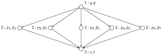
Figure 12. Construction of the DAG for the coNP-hardness proof for fit for backwards induction in the case of the formula φ being defined over five variables p₁ through p₅.

First, assume that $\phi$ is not satisfiable. Then, all players are indifferent between all outcomes, and it can easily be seen that the game is fit for backwards induction under $\tau$.

Finally, assume that assignment $\alpha :\{p_1,\cdots ,p_m\}\to \{0,1\}$ satisfies $\phi$. Observe that $v_q$ is inscrutable to $v_r$ and has a lower topological rank under $\tau$. Moreover, $v_{p_1},\cdots ,v_{p_m}$ are the parents of $v_r$. Now, let $a_{v_{p_1}},\cdots ,a_{v_{p_m}}$ be such that $a_{p_j}=p_j$ if $\alpha \left(p_j\right)=1$, and $a_{p_j}={\overline{p}}_j$ if $\alpha \left(p_j\right)=0$. Furthermore, let $b_{v_q}=q$ and $b_{v_q}^{\prime }=\overline{q}$, and $a_{v_r}=r$ and $a_{v_r}^{\prime }=\overline{r}$. Then,

$$u_3(q,a_{v_{p_1}},\cdots ,a_{v_{p_m}},r)>u_3(q,a_{v_{p_1}},\cdots ,a_{v_{p_m}},\overline{r})$$

but

$$u_3(\overline{q},a_{v_{p_1}},\cdots ,a_{v_{p_m}},r)<u_3(\overline{q},a_{v_{p_1}},\cdots ,a_{v_{p_m}},\overline{r}).$$

Accordingly, we may conclude that the game is not fit for backwards induction. □

The closely related decision problem of whether a given partial order game is of adequate information, can be formulated as follows.

adequate information
Given:	Partial order game G and topological sorting $\tau$
Problem:	Is G a game of adequate information under $\tau$?

Again, note that adequate information is vacuous for total-order games. For general partial order games, we find that the problem of adequate information is not easier than fit for backwards induction. The similarity of the two problems—and so also the closeness of the concepts of fitness of backwards induction and adequate information—is revealed by the closeness of their respective proofs of $\mathrm{coNP}$-completeness.

Theorem 10.

adequate informationis $\mathrm{coNP}$-complete.

Proof. 

For membership in $\mathrm{coNP}$, let a certificate for a counterexample consist of a player i, a pair of profiles ${\mathbf{a}}_S$ and ${\mathbf{a}}_S^{\prime }$ in ${\mathbf{A}}_S$, and a pair of profiles ${\mathbf{b}}_I$ and ${\mathbf{b}}_I^{\prime }$ in ${\mathbf{A}}_I$, where S is the set of vertices that are scrutable to i under $\tau$ and I the set of vertices that are inscrutable to i under $\tau$. Observe that such a certificate is of polynomial size and that the sets S and I can be computed in polynomial time. Then, such a certificate $({\mathbf{a}}_S,{\mathbf{a}}_S^{\prime },{\mathbf{b}}_I,{\mathbf{b}}_I^{\prime })$ defines a counterexample against the game being of adequate information whenever it is not the case that $u_i({\mathbf{a}}_S,{\mathbf{b}}_I)\le u_i({\mathbf{a}}_S^{\prime },{\mathbf{b}}_I)$ if and only if $u_i({\mathbf{a}}_S,{\mathbf{b}}_I^{\prime })\le u_i({\mathbf{a}}_S^{\prime },{\mathbf{b}}_I^{\prime })$. Having assumed that the utility function $u_i$ is part of the input and represented by a Boolean circuit and evaluation problem for Boolean circuits is solvable in polynomial time, we find that this is a property that can be checked in polynomial time (see Lemma 2).

The proof of $\mathrm{coNP}$-hardness is by a reduction from the complement of satisfiability, and runs along analogous lines as the proof of $\mathrm{coNP}$-hardness of fit for backwards induction. Thus, given a propositional formula $\phi$ in the variables $p_1,\cdots ,p_k$, construct the partial order Boolean game as in the proof of Theorem 9.

Then, if $\phi$ is not satisfiable, we find that for all three players, each action profile yields a utility of 1. It thus immediately follows that the game is of adequate information, as we can set, for instance, $u_i^0\left({\mathbf{a}}_S\right)=1$ for all players i with set S of scrutable vertices under $\tau$.

For the opposite direction, assume that assignment $\alpha :\{p_1,\cdots ,p_m\}\to \{0,1\}$ witnesses the satisfiability of $\phi$. Observe that $v_q$ is inscrutable to player 3 under $\tau$, whereas $v_q,v_{p_1},\cdots ,v_{p_m}$ are scrutable to player 3. Now let $a_{v_{p_1}},\cdots ,a_{v_{p_m}}$ be such that $a_{p_j}=p_j$ if $\alpha \left(p_j\right)=1$, and $a_{p_j}={\overline{p}}_j$ if $\alpha \left(p_j\right)=0$. Then,

$$u_3(q,a_{v_{p_1}},\cdots ,a_{v_{p_m}},r)>u_3(q,a_{v_{p_1}},\cdots ,a_{v_{p_m}},\overline{r})$$

but

$$u_3(\overline{q},a_{v_{p_1}},\cdots ,a_{v_{p_m}},r)<u_3(\overline{q},a_{v_{p_1}},\cdots ,a_{v_{p_m}},\overline{r}).$$

Assuming that the game be of adequate information, there then should be a utility function $u_3^0:{\mathbf{A}}_S\to \mathbb{R}$ such that from the former it would follow that $u_3^0(a_{v_{p_1}},\cdots ,a_{v_{p_m}},r)>u_3^0(a_{v_{p_1}},\cdots ,a_{v_{p_m}},\overline{r})$, whereas from the latter $u_3^0(a_{v_{p_1}},\cdots ,a_{v_{p_m}},r)<u_3^0(a_{v_{p_1}},\cdots ,a_{v_{p_m}},\overline{r})$, a contradiction. Accordingly, we may conclude that the game is not of adequate information. □

Using Theorems 7 and 8, we know that games that are fit for backwards induction, like games of adequate information, have Nash equilibria. Thus, Theorems 9 and 10 could be seen to prove $\mathrm{coNP}$-completeness of weak versions of the non-emptiness problem for backwards induction. This still leaves the question of whether a given strategy profile is a backwards induction solution and of whether a given action profile is sustained by a backwards induction solution, which can be seen as variants of the non-emptiness problem for backwards induction. The first decision problem can be formulated formally as follows.

is backward induction
Given:	Partial order game G that is fit for backwards induction under topological sorting $\tau$ and strategy profile $\mathbf{f}=(f_{v_1},\cdots ,f_{v_{\left|V\right|}})$
Problem:	Is $\mathbf{f}$ a backwards induction solution of G under $\tau$?

We find that is backward induction is $\mathrm{coNP}$-complete. For the membership part, recall that Lemma 5 showed that our backwards induction procedure has the one-stage-deviation property. Let $\tau$ be a topological sorted and assume $(v_1,\cdots ,v_{\left|V\right|})$ be sorted according to $\tau$. The contrapositive of the one-stage-deviation property says that, if a profile $\mathbf{f}$ is not a backwards induction solution, there is one player, who, after some $\tau$-history, wants to unilaterally deviate and play another action than the one prescribed by $\mathbf{f}$, but otherwise has no incentive to change their strategy. This prepares the ground for the following result.

Theorem 11.

is backward inductionis $\mathrm{coNP}$-complete. The problem remains $\mathrm{coNP}$-hard for total-order games.

Proof. 

For membership in $\mathrm{coNP}$, one can design a non-deterministic algorithm along the following lines. Assume $v_{v_1},\cdots ,v_{v_{\left|V\right|}}$ is ordered according to $\tau$. Guess a vertex $v_k$ assigned to player i along with action profiles $\mathbf{a}=({\mathbf{a}}_X,{\mathbf{a}}_Y,a_{v_k},{\mathbf{a}}_Z)$ and ${\mathbf{a}}^{\prime }=({\mathbf{a}}_X,{\mathbf{a}}_Y,a_{v_k}^{\prime },{\mathbf{a}}_Z^{\prime })$ (thus, ${\mathbf{a}}_X^{\prime }={\mathbf{a}}_X$ and ${\mathbf{a}}_Y^{\prime }={\mathbf{a}}_Y$). Let Y denote the parents of $v_k$, Z the vertices with a greater topological index than $v_k$, and $X=V\backslash (Y\cup Z\cup \left\{v_k\right\})$. Then, check whether

(i)

the actions $a_{v_k},a_{v_{k+1}}\cdots ,a_{v_{\left|V\right|}}$ are in accordance with $\mathbf{f}=(f_{v_1},\cdots ,f_{v_{\left|V\right|}})$, that is, for every $k\le m\le \left|V\right|$, we have $a_{v_m}=f_{v_m}\left({\mathbf{a}}_{Y_m}\right)$, where $Y_m$ is the set of parents of $v_m$;

(ii)

the actions $a_{v_{k+1}}^{\prime },\cdots ,a_{v_{\left|V\right|}}^{\prime }$ are in accordance with $\mathbf{f}=(f_{v_1},\cdots ,f_{v_{\left|V\right|}})$, that is, for every $k<m\le \left|V\right|$, we have $a_{v_m}^{\prime }=f_{v_m}({\mathbf{a}}_{Y_m}^{\prime })$, where $Y_m$ is the set of parents of $v_m$; and

(iii)

$u_i\left({\mathbf{a}}^{\prime }\right)>u_i\left(\mathbf{a}\right)$.

In virtue of Lemmas 1 and 2, each of these checks can be performed in polynomial time in the size of the input. Moreover, if all of these checks are positive, we have found a counterexample against $\mathbf{f}$ being a backwards induction solution.

For $\mathrm{coNP}$-hardness, we reduce the complement of satisfiability. Given an Boolean formula $\phi$ on propositional variables $p_1,\cdots ,p_k$, we construct a partial order Boolean game $G_{\phi }$ with one player i with goal formula ${\gamma }_i=\phi \wedge p_0$, where $p_0$ is a “fresh” variable distinct from any $p_1,\cdots ,p_k$. Let the vertices $v_{p_0},\cdots ,v_{p_k}$ be ordered accordingly, that is, $p_{\ell }E{p}_m$ if and only if $\ell <m$. Thus, $G_{\phi }$ is a totally-ordered Boolean game, and, consequently, also fit for backwards induction. Now, consider the strategy profile ${\mathbf{f}}^0=(f_{v_{p_0}}^0,\cdots ,f_{v_{p_k}}^0)$ where each $f_{v_{p_j}}^0$ is represented by the choice equation $p_j:\perp$, that is, ${\mathbf{f}}^0$ unconditionally sets every propositional variable to false. Note that ${\mathbf{f}}^0$ yields player i a utility of 0, that is $u_i\left({\mathbf{f}}^0\right)=0$.

Now, if $\phi$ is unsatisfiable, so is i’s goal ${\gamma }_i$, and all strategy profiles yield i the same payoff. Therefore, ${\mathbf{f}}^0$ is vacuously a backwards induction solution. If, on the other hand, $\phi$ is satisfiable, say in virtue of assignment $\alpha$, let ${\mathbf{f}}^{\alpha }=(f_{v_{p_0}},\cdots ,v_{p_k})$ be the unconditional strategy profile represented by the choice equations $p_0=\top$ and, for each $1\le m\le k$, $p_m:\top$, if $\alpha \left(p_m\right)=1$, and $p_m:\perp$, if $\alpha \left(p_m\right)=0$. It can then easily be verified that player i has $u_i\left({\mathbf{f}}^{\alpha }\right)=1$. Accordingly, player i has an incentive to deviate from ${\mathbf{f}}^0$ to ${\mathbf{f}}^{\alpha }$, indicating that ${\mathbf{f}}^0$ is not a Nash equilibrium. By Theorem 7, it then follows that ${\mathbf{f}}^0$ is not a backwards induction solution either. □

Finally, we come to consider the natural counter-part of the is nash actions problem for the backwards induction procedure, which can formally be stated as follows.

is backward induction actions
Given:	Partial order game G, topological sorting $\tau$, and action profile $\mathbf{a}=(a_{v_1},\cdots ,a_{v_{\left|V\right|}})$
Problem:	Is $\mathbf{a}$ sustained by a backwards induction solution under $\tau$ in G?

We find that backwards induction actions is $\mathrm{NEXPTIME}$-complete for general partial order games. The hardness part of this result follows again from a reduction from dependency quantifier boolean formula game (dqbfg).

Theorem 12.

For partial order games,backward induction actionsis $\mathrm{NEXPTIME}$-complete.

Proof. 

A $\mathrm{NEXPTIME}$ algorithm to decide backward induction actions can be designed along the following lines. Given a partial order game G, a topological-ordering $\tau =(v_1,\cdots ,v_{\left|V\right|})$ of its vertices, and an action profile $\mathbf{a}=(a_{v_1},\cdots ,a_{v_{\left|V\right|}})$, first, guess a strategy profile $\mathbf{f}=(f_{v_1},\cdots ,f_{v_{\left|V\right|}})$. Given that strategies $f_v$ are given by a Boolean circuit ${\mathbb{C}}_{f_v}$, this can be achieved in time not more than exponential in $\left|A\right|$, the size of the set of actions. Second, check whether $\mathbf{f}=(f_{v_1},\cdots ,f_{v_{\left|V\right|}})$ is a backwards induction solution. The inductive definition of a backwards induction solution suggests a procedure for how this can be achieved in exponential time. Finally, check whether action profile ${\mathbf{a}}^{\mathbf{f}}$ as induced by strategy profile $\mathbf{f}$ coincides with the action profile $\mathbf{a}$ as it is given in the input. This can be achieved in time polynomial in the size of the Boolean circuit representing $\mathbf{f}$. Altogether, the algorithm runs in non-deterministic exponential time.

For hardness, we reduce from dependency quantifier boolean formula game (dqfg) using a similar construction of a Boolean partial order game as in the proof of Theorem 4. Given an instance $⟨\phi ,X_1,X_2,Y_1,Y_2⟩$ of dqfg with $X_1=\{x_1^1,\cdots ,x_{|X_1|}^1\}$, $X_2=\{x_1^2,\cdots ,x_{|X_2|}^2\}$, $Y_1=\{y_1^1,\cdots ,y_{|Y_1|}^1\}$, and $Y_2=\{y_1^2,\cdots ,y_{|Y_2|}^2\}$. Let $x_0$ be a ‘fresh’ variable $x_0$ not in $X_1\cup X_2\cup Y_1\cup Y_2$. We define a Boolean partial order game on dependency graph $(V,E)$ such that $V=\left\{x_0\right\}\cup X_1\cup X_2\cup Y_1\cup Y_2$ and where E is defined as follows:

(i)

$x_{0}Ez$   for all $z\in X_1\cup X_2\cup Y_1\cup Y_2$,

(ii)

$x_k^{i}E{x}_m^j$  for all $x_k^i\in X_i$ and $x_m^j\in X_j$ with $i=j$ and $k<m$, or $i\le j$,

(iii)

$x_{1}E{x}_2$, for all $x_1\in X_1$ and $x_2\in X_2$,

(iv)

$x_{1}E{y}_1$, for all $x_1\in X_1$ and $y_1\in Y_2$,

(v)

$x_{2}E{y}_2$, for all $x_2\in X_2$ and $y_2\in Y_2$.

Observe that under this definition on $X_1\cup X_2$, the relation E is complete and transitive. We extend E to a topological sorting $\tau$ such that, for instance,

$$\tau =(x_0,x_1^1,\cdots ,x_{|X_1|}^1,x_1^2,\cdots ,x_{|X_2|}^2,y_1^1,\cdots ,y_{|Y_1|}^1,y_1^2,\cdots ,y_{|Y_2|}^2).$$

The players of the Boolean game are the same as in the instance of dqbfg, where B controls $\left\{x_0\right\}\cup X_1\cup X_2$, $W_1$ the variables in $Y_1$, and $W_2$ those in $Y_2$. Their goals are given by

$$\begin{array}{cccc}\hfill {\gamma }_B& =x_0\wedge \phi \hfill & \hfill {\gamma }_{W_1}& ={\gamma }_{W_2}=\perp .\hfill \end{array}$$

Observe that all vertices are scrutable to player B under $\tau$ and that the white players have the same utility for every outcome. It therefore follows that the game constructed is of adequate information and hence fit for backwards induction.

We are now in a position to show that the profile

$$\overline{\mathbf{a}}=({\overline{x}}_0,{\overline{x}}_1^1,\cdots {\overline{x}}_{|X_1|}^1,{\overline{x}}_1^2\cdots ,{\overline{x}}_{|X_2|}^2,{\overline{y}}_1^2,\cdots {\overline{y}}_{|Y_1|}^1,{\overline{y}}_1^2\cdots ,{\overline{y}}_{|Y_2|}^2),$$

which sets all variables, including $x_0$, to false, is sustained by a Nash equilibrium in $G^{\prime }$ if and only if $⟨\phi ,X_1,X_2,Y_1,Y_2⟩$ is a postive instance of dqbfg.

First, assume $⟨\phi ,X_1,X_2,Y_1,Y_2⟩$ is a postive instance of dqbfg. Then, the white team has a joint winning strategy in the original dqbfg-game given by Boolean functions ${\beta }_1$ and ${\beta }_2$ on the variables $X_1$ and $X_2$, respectively. Next, define strategies ${\mathbf{f}}_{W_1}^{*}$ and ${\mathbf{f}}_{W_2}^{*}$ for $W_1$ and $W_2$ in the Boolean partial order game that are given by the following choice equations for $i=1,2$ and $j=1,\cdots ,|Y_i|$,

$$y_j^i:(x_0\to {\phi }_{{\beta }_i}(x_1^i,\cdots ,x_{|X_i|}^i))\wedge ({\overline{x}}_0\to \perp )$$

As the dependency graph $(V,E)$ respects the information dependencies of the dqbfg-instance, observe that ${\mathbf{f}}_{W_1}$ and ${\mathbf{f}}_{W_2}$ together embody a winning strategy to render $\phi$ false if $x_0$ is played. Let B’s unconditional strategy ${\mathbf{f}}_B^{*}$ be defined by the choice equations of the form $x_j^i:\perp$, setting $x_j^i$ to false for all for $i=1,2$ and $j=1,\cdots ,|X_i|$. Observe that for the strategy profile ${\mathbf{f}}^{*}=({\mathbf{f}}_B^{*},{\mathbf{f}}_{W_1}^{*},{\mathbf{f}}_{W_2}^{*})$, we have that ${\mathbf{a}}^{{\mathbf{f}}^{*}}=\overline{\mathbf{a}}$, as desired. As $W_1$ and $W_2$ will not have their goal achieved under any action profile, their strategies trivially conform with the backwards induction procedure. Observe furthermore that B does not get their goal satisfied no matter which strategy plays against ${\mathbf{f}}_{W_1}^{*}$ and ${\mathbf{f}}_{W_2}^{*}$. If B sets $x_0$ to false, their goal is not satisfied in a self-defeating fashion. By setting $x_0$ to true, B will induce $W_1$ and $W_2$ to play a winning strategy rendering $\neg \phi$ false and therewith ${\gamma }_B$ as well. This in particular holds for any backwards induction strategies B has at their disposal, and it follows that ${\mathbf{f}}^{*}$ is a backwards induction solution sustaining $\overline{\mathbf{a}}$.

For the opposite direction, assume that $⟨\phi ,X_1,X_2,Y_1,Y_2⟩$ is a negative instance of dqbfg. Analogously to the proof of Theorem 4, it can then be shown that the constructed partial order Boolean game does not have a Nash equilibrium sustaining $\overline{\mathbf{a}}$. In virtue of the contrapositive of Theorem 7, there is no backwards induction solution sustaining $\overline{\mathbf{a}}$, giving us the result. □

The computational complexity of backward induction actions reduces considerably when we restrict attention to total-order games. Still, the problem is $\mathrm{PSPACE}$-complete for this class of games. To prove this result, we first introduce some auxiliary notation and terminology.

Recall that if the dependency graph $(V,E)$ of a total-order game is such that $v_{0}E\cdots E{v}_{\left|V\right|}$, then $\tau =(v_0,\cdots ,v_{\left|V\right|})$ is the only topological sorting of the vertices. Moreover, the parents of each vertex $v_k$ are all vertices with a lower topological index. The set $\{v_1,\cdots ,v_{k-1}\}$ of parents of vertex $v_k$ we will denote by $Y_k$, on the understanding that $Y_k=Ø$, if $k=0$. Similarly, we will denote by $Z_k=\{v_{k+1},\cdots ,v_{\left|V\right|}\}$ the set of vertices with a higher topological index than $v_k$, here on the understanding that $Z_k=Ø$, if $k=\left|V\right|$.

For $\mathbf{a}=(a_{v_1},\cdots ,a_{v_{\left|V\right|}})$ an action profile and $\mathbf{h}=(a_{v_1},\cdots ,a_{v_k})$ a $\tau$-history of $\mathbf{a}$, we now introduce the auxiliary concept of $\mathbf{a}$ being sustained by a backwards induction solution at history h of a. This enables us to reason recursively about action profiles being sustained by backwards induction solutions without having to make explicit reference to specific underlying strategy profiles. Formally, for action profile $\mathbf{a}= (a_{v_1},\cdots ,a_{v_{\left|V\right|}})$ $and$ τ-history $\mathbf{h}= (a_{v_1},\cdots ,a_{v_k})$ of a we say that a is sustained (by backwards induction) at h, if either h = a, or $\mathbf{h}= (a_{v_1},\cdots ,a_{v_k})$ for some 0 < k < |V| and the following two conditions hold:

(a.i)

action profile a is sustained by backwards induction at history $(a_{v_1},\cdots ,a_{v_k},a_{v_{k+1}})$

(a.ii)

for every $b_{v_{k+1}}\in A_{v_{k+1}}$, there is an action profile ${\mathbf{a}}^{\prime }=(a_{v_1},\cdots ,a_{v_k},b_{v_{k+1}},b_{v_{k+2}}\cdots ,b_{v_{\left|V\right|}})$ that is sustained by backwards induction at history $(a_{v_1},\cdots ,a_{v_k},b_{v_{k+1}})$ and which is such that $u_i\left(\mathbf{a}\right)\ge u_i\left({\mathbf{a}}^{\prime }\right)$, where i is the player active at v_k+1.

We now have the following lemma.

Lemma 7.

For total-order games, an action profile$\mathbf{a}=(a_{v_1},\cdots ,a_{v_{\left|V\right|}})$is sustained by a backwards induction solution if and only if$\mathbf{a}$is sustained by backwards induction at all histories of$\mathbf{a}$. Moreover,$\mathbf{a}$is sustained by a backwards induction solution only if$\mathbf{a}$is sustained by backwards induction at the empty history$\left(\right)$.

Proof. 

As we are dealing with total-order games, first observe that, for each vertex v, the set X of vertices that are neither a parent of v nor have a greater topological index than v is empty. Thus, Condition (1) in the definition of a backwards induction solution ${\mathbf{f}}^{*}$ for partial order games reduces to

$$f_{v_{k+1}}^{*}(a_{v_1},\cdots ,a_{v_k})\in \underset{b_{v_{k+1}}\in A_{v_{k+1}}}{arg\; max}{u}_i(a_{v_1},\cdots ,a_{v_k},b_{v_{k+1}},f_{v_{k+2}},\cdots ,f_{v_{\left|V\right|}}),$$

(BI″)

for all $0\le k<\left|V\right|$, and where i is the player active at $v_{k+1}$.

As an auxiliary concept, we define a strategy profile $\mathbf{f}=(f_{v_1},\cdots ,f_{v_{\left|V\right|}})$ to sustain action profile $\mathbf{a}=(a_{v_1},\cdots ,a_{v_{\left|V\right|}})$ (by backwards induction) at history $\mathrm{h}=(a_{v_1},\cdots ,a_{v_k})$, if either $\mathbf{a}=\mathbf{h}$, or both

(f.i)

f sustains a at $(a_{v_1},\cdots ,a_{v_k},a_{v_{k+1}})$,

(f.ii)

$f_{v_{k+1}}(a_{v_1},\cdots ,a_{v_k})=a_{v_{k+1}}$, and

(f.iii)

for all $b_{v_{k+1}}\in A_{v_{k+1}}$ with $b_{v_{k+1}}\ne a_{v_{k+1}}$ we have that f sustains action profile $(a_{v_1},\cdots ,a_{v_k},b_{v_{k+1}},f_{v_{k+2}},\cdots ,f_{v_{\left|V\right|}})$ at history $(a_{v_1},\cdots ,a_{v_k},b_{v_{k+1}})$ and,

$$u_i(a_{v_1},\cdots ,a_{v_k},a_{v_{k+1}},a_{v_{k+2}}\cdots ,a_{v_{\left|V\right|}})\ge u_i(a_{v_1},\cdots ,a_{v_k},b_{v_{k+1}},f_{v_{k+1}},\cdots ,f_{v_{\left|V\right|}}),$$

where i is the player active at $v_{k+1}$.

The we split the proof up in three parts, where we prove, respectively, the following statements (I), (II), and (III), below. In conclusion then put them together again, to prove the lemma.

(I)

for all $0\le k\le \left|V\right|$ and all action profiles $\mathbf{a}=(a_{v_1},\cdots ,a_{v_{\left|V\right|}})$, $\mathbf{a}$ is sustained at $(a_{v_1},\cdots ,a_{v_k})$ if and only if some strategy profile $\mathbf{f}=(f_{v_1},\cdots ,f_{v_{\left|V\right|}})$ sustains $\mathbf{a}$ at $(a_{v_1},\cdots ,a_{v_k})$.

(II)

strategy profile $\mathbf{f}=(f_{v_1},\cdots ,f_{v_{\left|V\right|}})$ sustains action profile $\mathbf{a}=(a_{v_1},\cdots ,a_{v_{\left|V\right|}})$ at history $\left(\right)$ if and only if ${\mathbf{a}}^{\mathbf{f}}=\mathbf{a}$ and for every $0\le k\le \left|V\right|$ and all action profiles $\mathbf{x}=(x_{v_1},\cdots ,x_{v_k},f_{v_{k+1}},\cdots ,f_{v_{\left|V\right|}})$, strategy profile $\mathbf{f}$ sustains $\mathbf{x}$ at $(x_{v_1},\cdots ,x_{v_k})$.

(III)

for every $0\le k\le \left|V\right|$ and every action profile ${\mathbf{x}}^{\prime }=(x_{v_1},\cdots ,x_{v_k},f_{v_{k+1}},\cdots ,f_{v_{\left|V\right|}})$, strategy profile $\mathbf{f}$ sustains $\mathbf{x}$ at history $\mathbf{h}=(x_{v_1},\cdots ,x_{v_k})$ if and only if strategy profile $\mathbf{f}=(f_{v_1},\cdots ,f_{v_{\left|V\right|}})$ is a backwards induction solution.

Part (I) is by induction on $\left|V\right|-k$. For the basis, where $k=\left|V\right|$, consider an arbitrary action profile $\mathbf{a}=(a_{v_1},\cdots ,a_{v_{\left|V\right|}})$ and arbitrary history $\mathbf{h}=(a_{v_1},\cdots ,a_{v_k})$. In this case, we find that $\mathbf{h}=\mathbf{a}$ and immediately that $\mathbf{a}$ is sustained at $\mathbf{h}$. Moereover, every strategy profile sustains $\mathbf{a}$ at $\mathbf{h}$ in this case.

For the induction step, consider an arbitrary $1\le k<\left|V\right|$, and equally arbitrary action profile $\mathbf{a}=(a_{v_1},\cdots ,a_{v_{\left|V\right|}})$ and history $\mathbf{h}=(a_{v_1},\cdots ,a_{v_k})$.

First, assume that $\mathbf{a}$ is sustained at $(a_{v_1},\cdots ,v_k)$, and let i be the player active at $v_{k+1}$. Then, $\mathbf{a}$ is also sustained at $(a_{v_1},\cdots ,v_{k+1})$. By the induction hypothesis, there is a strategy profile $\mathbf{f}$ that sustains $\mathbf{a}$ at $(a_{v_1},\cdots ,v_{k+1})$. Moreover, as $k<\left|V\right|$, for each $b_{v_k+1}\in A_{v_k}$ with $b_{v_{k+1}}\ne a_{v_{k+1}}$, there is an action profile ${\mathbf{a}}^{\prime }=(a_{v_1},\cdots ,a_{v_{k1}},b_{v_{k+1}},b_{v_{k+2}}\cdots ,b_{v_{\left|V\right|}})$ that is sustained at history $(a_{v_1},\cdots ,a_{v_{k-1}},b_{v_k},b_{v_{k+1}})$ such that $u_i\left(\mathbf{a}\right)\ge u_i\left({\mathbf{a}}^{\prime }\right)$. Let $A_{v_{k+1}}=\{b_{v_{k+1}}^1,\cdots ,b_{v_{k+1}}^{|A_{v_{k+1}}|}\}$. By the induction hypothesis, for each $1\le j\le |A_{v_{k+1}}|$, there is a strategy profile ${\mathbf{g}}^j=(g_{v_1}^j,\cdots ,g_{v_{\left|V\right|}}^j)$ sustaining action profile $(a_{v_1},\cdots ,a_{v_k},b_{v_{k+1}}^j,g_{v_{k+2}}^j\cdots ,g_{v_{\left|V\right|}}^j)$ at history $(a_{v_1},\cdots ,a_{v_k},b_{v_{k+1}}^j)$, and which is such that

$$u_i\left(\mathbf{a}\right)\ge u_i(a_{v_1},\cdots ,a_{v_k},b_{v_{k+1}}^j,g_{v_{k+1}}^j,\cdots ,g_{v_{\left|V\right|}}^j).$$

Now, define the strategy profile ${\mathbf{f}}^{*}=(f_{v_1}^{*},\cdots ,f_{v_{\left|V\right|}}^{*})$ such that for $1\le k\le \left|V\right|$ and every history $\mathbf{x}=(x_{v_1},\cdots ,x_m)$, where $0\le m\le \left|V\right|$,

$$f_{v_m}^{*}\left(\mathbf{x}\right)=\left\{\begin{array}{cc}{f}_{v_m}^j\left(\mathbf{x}\right)\hfill & \mathrm{if}{x}_{v_{k+1}}=a_{v_{k+1}}^j\mathrm{and}m>k,\hfill \\ g_{v_m}^j\left(\mathbf{x}\right)\hfill & \mathrm{if}{x}_{v_{k+1}}=b_{v_{k+1}}^j\mathrm{and}m>k,\hfill \\ a_{v_m}\hfill & \mathrm{otherwise}.\hfill \end{array}\right.$$

It is now easy to check that, by construction, strategy profile ${\mathbf{f}}^{*}$ sustains $\mathbf{a}$ at history $(a_{v_1},\cdots ,a_{v_k})$, as desired. In particular, observe that $f_{v_{k+1}}^{*}(a_{v_1},\cdots ,a_{v_k})=a_{v_{k+1}}$.

For the opposite direction, assume that strategy profile $\mathbf{f}=(f_{v_1},\cdots ,f_{v_{\left|V\right|}})$ sustains action profile $\mathbf{a}=(a_{v_1},\cdots ,a_{v_{\left|V\right|}})$ at history $(a_{v_1},\cdots ,a_{v_k})$, where $k<\left|V\right|$. Then, by definition, strategy profile $\mathbf{f}=(f_{v_1},\cdots ,f_{v_{\left|V\right|}})$ also sustains action profile $\mathbf{a}=(a_{v_1},\cdots ,a_{v_{\left|V\right|}})$ at history $(a_{v_1},\cdots ,a_{v_{k=1}})$. By the induction hypothesis, we then immediately obtain that $\mathbf{a}$ is sustained at history $(a_{v_1},\cdots ,a_{v_{k+1}})$. Now, consider an arbitrary $b_{v_{k+1}}\in A_{v_{k+1}}$ with $a_{v_{k+1}}\ne b_{v_{k+1}}$, along with history $(a_{v_1},\cdots ,a_{v_k},b_{v_{k+1}})$. Then, $\mathbf{f}$ sustains action profile $(a_{v_1},\cdots ,a_{v_k},b_{v_{k+1}},f_{v_{k+2}},\cdots ,f_{v_{\left|V\right|}})$ at history $(a_{v_1},\cdots ,a_{v_k},b_{v_{k+1}})$. We have, moreover, that $u_i\left(\mathbf{a}\right)\ge u_i((a_{v_1},\cdots ,a_{v_k},b_{v_{k+1}},f_{v_{k+2}},\cdots ,f_{v_{\left|V\right|}}))$. By the induction hypothesis, we find that action profile $(a_{v_1},\cdots ,a_{v_k},b_{v_{k+1}},f_{v_{k+2}},\cdots ,f_{v_{\left|V\right|}})$ is sustained at history $(a_{v_1},\cdots ,a_{v_k},b_{v_{k+1}})$, which proves the case.

For part (II), first assume that ${\mathbf{a}}^{\mathbf{f}}=\mathbf{a}$ and that for every $0\le k\le \left|V\right|$, strategy profile $\mathbf{f}$ sustains action profile $(x_{v_1},\cdots ,x_{v_k},f_{v_{k+1}},\cdots ,f_{v_{\left|V\right|}})$ at history $(x_{v_1},\cdots ,x_{v_k})$. The latter then holds in particular for $k=0$, that is, for history $\left(\right)$. Accordingly, $\mathbf{f}$ sustains action profile $(f_{v_1},\cdots ,f_{v_{\left|V\right|}})={\mathbf{a}}^{\mathbf{f}}$ at history $\left(\right)$. Our initial assumption that ${\mathbf{a}}^{\mathbf{f}}$ then gives the result for this direction.

For the opposite direction, assume that strategy profile $\mathbf{f}=(f_{v_1},\cdots ,f_{v_{\left|V\right|}})$ sustains action profile $\mathbf{a}=(a_{v_1},\cdots ,a_{v_{\left|V\right|}})$ at history $\left(\right)$. First, we find that by repeatedly applying condition (f.ii) gives us ${\mathbf{a}}^{\mathbf{f}}=\mathbf{a}$. Now, consider an arbitrary $0\le k\le \left|V\right|$ and action profile $\mathbf{x}=(x_{v_1},\cdots ,x_{v_k},f_{v_{k+1}},\cdots ,f_{v_{\left|V\right|}})$. We prove by induction on k that $\mathbf{f}$ sustains $(x_{v_1},\cdots ,x_{v_k},f_{v_{k+1}},\cdots ,f_{v_{\left|V\right|}})$ at history $\mathbf{h}=(x_{v_1},\cdots ,x_{v_k})$.

First assume that $k=0$, that is, $\mathbf{h}=\left(\right)$. In that case, $\mathbf{x}=(f_{v_1},\cdots ,f_{v_{\left|V\right|}})={\mathbf{a}}^{\mathbf{f}}$. We have already seen that ${\mathbf{a}}^{\mathbf{f}}=\mathbf{a}$, and, thus, the base case immediately follows from the assumption that $\mathbf{f}=(f_{v_1},\cdots ,f_{v_{\left|V\right|}})$ sustains action profile $\mathbf{a}=(a_{v_1},\cdots ,a_{v_{\left|V\right|}})$ at history $\left(\right)$.

For the induction step, let $k>0$. In case $k=\left|V\right|$ we have $\mathbf{h}=\mathbf{a}$ and we are done immediately. Otherwise, by the induction hypothesis, we may assume that $\mathbf{f}$ sustains action profile $(x_{v_1},\cdots ,x_{v_{k-1}},f_{v_k},\cdots ,f_{v_{\left|V\right|}})$ at history $(x_{v_1},\cdots ,x_{v_{k-1}})$. If $f_{v_k}(x_{v_1},\cdots ,x_{v_{k-1}})=x_k$, then it follows from condition (f.i) that $\mathbf{f}$ sustains $(x_{v_1},\cdots ,x_{v_k},f_{v_{k+1}},\cdots ,f_{v_{\left|V\right|}})$ at $(x_{v_1},\cdots ,x_{v_k})$. If $f_{v_k}(x_{v_1},\cdots ,x_{v_{k-1}})\ne x_k$, then still $f_{v_k}(x_{v_1},\cdots ,x_{v_{k-1}})\in A_{v_k}$. Now, it follows from condition (f.iii) that $\mathbf{f}$ sustains $(x_{v_1},\cdots ,x_{v_k},f_{v_{k+1}},\cdots ,f_{v_{\left|V\right|}})$ at $(x_{v_1},\cdots ,x_{v_k})$.

For part (III), first assume, for every $0\le k\le \left|V\right|$ and action profile $\mathbf{x}=(x_{v_1},\cdots ,x_{v_k},f_{v_{k+1}},$$\cdots ,f_{v_{\left|V\right|}})$, that strategy profile $\mathbf{f}=(f_{v_1},\cdots ,f_{v_{\left|V\right|}})$ sustains $\mathbf{x}$ at history $\mathbf{h}=(x_{v_1},\cdots ,x_{v_k})$. Now, consider an arbitrary history $(z_1,\cdots ,z_k)$ for some $1\le k<\left|V\right|$. Then, by assumption, $\mathbf{f}$ sustains action profile $(z_{v_1},\cdots ,z_{v_k},f_{v_{k+1}},\cdots ,f_{v_{\left|V\right|}})$ at history $(z_{v_1},\cdots ,z_{v_k})$. As $k<\left|V\right|$, we find that $(z_1,\cdots ,z_k)\ne (z_1,\cdots ,z_k,f_{v_{k+1}},\cdots ,f_{v_{\left|V\right|}})$. Therefore, by condition (f.iii), we then find that

$$f_{v_{k+1}}(z_{v_1},\cdots ,z_{v_k})\in \underset{b_{v_{k+1}}\in A_{v_{k+1}}}{arg\; max}{u}_i(z_{v_1},\cdots ,z_{v_k},b_{v_{k+1}},f_{v_{k+2}},\cdots ,f_{v_{\left|V\right|}}),$$

where i is the player active at $v_{k+1}$. It thus follows that $\mathbf{f}$ is a backward induction solution.

For the opposite direction, assume that $\mathbf{f}=(f_{v_1},\cdots ,f_{v_{\left|V\right|}})$ is a backwards induction solution. Now, consider an arbitrary $0\le k\le \left|V\right|$. We prove by induction on $\left|V\right|-k$, that, for every action profile $\mathbf{x}=(x_{v_1},\cdots ,x_{v_k},f_{v_{k+1}},\cdots ,f_{v_{\left|V\right|}})$, strategy profile $\mathbf{f}$ sustains $\mathbf{x}$ at history $\mathbf{h}=(x_{v_1},\cdots ,x_{v_k})$.

For the basis assume let $k=\left|V\right|$. Consider an arbitrary action profile $\mathbf{x}=(x_{v_1},\cdots ,x_{v_k})$ along with history $\mathbf{h}=(x_{v_1},\cdots ,x_{v_k})$. Obviously, $\mathbf{h}=\mathbf{x}$, and, thus, immediately that $\mathbf{f}$ sustains $\mathbf{x}$ at history h.

For the induction step, let $k<\left|V\right|$. Again, consider an arbitrary action profile $\mathbf{h}=(x_{v_1},\cdots ,x_{v_k},f_{v_{k+1}},\cdots ,f_{v_{\left|V\right|}})$ along with history $\mathbf{h}=(x_{v_1}x\cdots ,x_{v_k})$. By the induction hypothesis, we find, for all action profiles $\mathbf{y}=(y_{v_1},\cdots ,y_{v_{k+1}},f_{v_{k+1}},\cdots ,f_{v_{\left|V\right|}})$, that $\mathbf{f}$ sustains $\mathbf{y}$ at history $(y_{v_1},\cdots ,y_{v_{k+1}})$. This holds in particular for histories $(x_{v_1},\cdots ,x_{v_k},b_{v_{k+1}})$ where $b_{v_{k+1}}\in A_{v_{k+1}}$. For $b_{v_{k+1}}=f_{v_{k+1}}(x_{v_1},\cdots ,f_{v_k})$, we obtain condition (f.i). Condition (f.ii) is trivially satisfied. Finally, having assumed that $\mathbf{f}$ is a backwards induction solution, we find that,

$$u_i(x_{v_1},\cdots ,x_{v_k},f_{v_{k+1}},f_{v_{k+2}},\cdots ,f_{v_{\left|V\right|}})\ge u_i(x_{v_1},\cdots ,x_{v_k},b_{v_{k+1}},f_{v_{k+2}},\cdots ,f_{v_{\left|V\right|}}),$$

for all $b_{v_{k+1}}\in V_{v_{k+1}}$ with $b_{v_{k+1}}\ne f_{v_{k+1}}(x_{v_1},\cdots ,f_{v_k})$ and i the player active at $v_{k+1}$. We may therefore conclude that $\mathbf{f}$ sustains $\mathbf{x}=(x_{v_1},\cdots ,x_{v_k},f_{v_{k+1}},\cdots ,f_{v_{\left|V\right|}})$ at $(x_{v_1},\cdots ,x_{v_k})$, proving part (III).

With (I) through (III) in place, we conclude the proof as follows. Consider an arbitrary action profile $\mathbf{a}=(a_{v_1},\cdots ,a_{v_{\left|V\right|}})$. First, assume, for all $0\le k\le \left|V\right|$, that $\mathbf{a}$ is sustained by backwards induction at $(a_{v_1},\cdots ,a_{v_k})$. Then by (I), for all $0\le k\le \left|V\right|$, there is some strategy profile $\mathbf{f}=(f_{v_1},\cdots ,f_{v_{\left|V\right|}})$ that sustains $\mathbf{a}$ by backwards induction at $(a_{v_1},\cdots ,a_{v_k})$. For the particular case wherein $k=0$, we find that this strategy profile $\mathbf{f}$ that sustains $\mathbf{a}$ by backwards induction at $\left(\right)$. By repeated application of (f.ii), moreover, it can easily be established that ${\mathbf{a}}^{\mathbf{f}}=\mathbf{a}$. Part (II) then yields that for every $0\le k\le \left|V\right|$ and all action profiles $\mathbf{x}=(x_{v_1},\cdots ,x_{v_k},f_{v_{k+1}},\cdots ,f_{v_{\left|V\right|}})$, strategy profile $\mathbf{f}$ sustains $\mathbf{a}$ at history $(x_{v_1},\cdots ,x_{v_k})$. Finally, by virtue of (III), we may conclude that $\mathbf{f}$ is a backwards induction solution that sustains $\mathbf{a}$.

For the opposite direction, assume that $\mathbf{f}$ is a backwards induction solution sustaining $\mathbf{a}$. Therefore, ${\mathbf{a}}^{\mathbf{f}}=\mathbf{a}$, and, accordingly, $(a_{v_1},\cdots ,a_{v_k},f_{v_{k+1}},\cdots ,f_{v_{\left|V\right|}})=(a_{v_1},\cdots ,a_{v_{\left|V\right|}})$ for all $0\le k\le \left|V\right|$. Part (III) yields furthermore that for every $0\le k\le \left|V\right|$, strategy profile $\mathbf{f}$ sustains action profile ${\mathbf{a}}^{\prime }=(a_{v_1},\cdots ,a_{v_k},f_{v_{k+1}},\cdots ,f_{v_{\left|V\right|}})$ at history $(a_{v_1},\cdots ,a_{v_k})$. It now follows, for every $0\le k\le \left|V\right|$, that $\mathbf{f}$ sustains $\mathbf{a}$ at history $(a_{v_1},\cdots ,a_{v_k})$. With part (I), we may now conclude that, for all $0\le k\le \left|V\right|$, action profile $\mathbf{a}$ is sustained by backwards induction at $(a_{v_1},\cdots ,a_{v_k})$, as desired.

Finally, observe that the second part of the lemma also follows from the above argument. □

The intuition behind Lemma is that, for a strategy profile $\mathbf{f}$ sustaining an action profile $\mathbf{a}=(a_{v_1},\cdots ,a_{v_{\left|V\right|}})$ to be a backward induction solution, it does not suffice just to induce $\mathbf{a}$, in the sense that ${\mathbf{a}}^{\mathbf{f}}=\mathbf{a}$. It should, in addition, incorporate a threat strategy at every vertex $v_k$ that succeeds in deterring the player active at $v_k$ to play any action other than $a_{v_k}$, that is, the action prescribed by $\mathbf{a}$. The lemma, moreover, shows that a strategy profile that achieve this can be constructed from the strategy profiles that achieve this at each history.

We introduce the following auxiliary decision problem, solving which is an important subroutine in our proof of $\mathrm{PSPACE}$-membership of backwards induction actions for total-order games.

backward induction guarantee
Given:	Total-order game G, action profiles $\mathbf{a}=(a_{v_1},\cdots ,a_{v_{\left|V\right|}})$ and history $\mathbf{h}=(a_{v_1},\cdots ,a_{v_k})$, player i, and $r\in \mathbb{R}$.
Problem:	Is $\mathbf{a}$ sustained by backwards induction at  h such that $u_i\left(\mathbf{a}\right)\le r$

We find that backward induction guarantee is in $\mathrm{PSPACE}$ for total-order games.

Lemma 8.

For total-order games,backward induction guaranteeis in $\mathrm{PSPACE}$, that is, the problem can be solved in space polynomial in the size of the game.

Proof. 

Let a total-order game be given together with an action profile $\mathbf{a}=(a_{v_1},\cdots ,a_{v_{\left|V\right|}})$. We prove by induction on $\left|V\right|-k$, that for all histories $\mathbf{h}=(a_{v_1},\cdots ,a_{v_k})$ of $\mathbf{a}$, all players i, and all values $r\in \mathbb{R}$ the problem backward induction guarantee can be solved in polynomial space.

For the basis, assume $k=\left|V\right|$. Then, $\mathbf{h}=\mathbf{a}$, and consider an arbitrary player i and arbitrary value $r\in \mathbb{R}$. In this case, it suffices to compute $u_i\left(\mathbf{a}\right)$ and check whether $u_i\left(\mathbf{a}\right)\le r$. By Lemma 2, this achieved in polynomial time, and hence in polynomial space as well.

For the induction step, let $k<\left|V\right|$. Consider an arbitrary player j and an arbitrary value $r\in \mathbb{R}$. Let, furthermore, i be the player active at $a_{v_k}$. Now, we first check whether $\mathbf{a}$ is sustained by backward induction at history ${\mathbf{h}}_{v_{k+1}}=(a_{v_1},\cdots ,a_{v_{k+1}})$. By virtue of the induction hypothesis, this can be achieved in polynomial space by computing backward induction guarantee for $\mathbf{a}$, history ${\mathbf{h}}_{v_{k+1}}$, player i, and value $r=u_i\left(\mathbf{a}\right)$. If this check is negative, we can conclude immediately and output “no”.

Otherwise, we deploy two binary counters with, respectively, ${log}_2\left|A\left(x\right)\right|$ and ${log}_2\left|H\right|=O\left(\right|V|{log}_2\left|A\right|)$ digits to run through all actions $b_{v_{k+1}}$ in $A_{v_k}$ and all action profiles

$$(a_{v_1},\cdots ,a_{v_k},b_{v_{k+1}},b_{k+1}^{\prime }\cdots ,b_{v_{\left|V\right|}}^{\prime }),$$

respectively. We then subsequently check for each $b_{v_{k+1}}$ in $A_{v_{k+1}}$ whether some action profile $\mathbf{b}=(a_{v_1},\cdots ,a_{v_k},b_{v_{k+1}},b_{k+1}^{\prime }\cdots ,b_{v_{\left|V\right|}}^{\prime })$ is sustained by backwards induction at $(a_{v_1},\cdots ,a_{v_k},$$b_{v_{k+1}})$ with $u_i\left(\mathbf{b}\right)\le u_i\left(\mathbf{a}\right)$. Then, $\mathbf{a}$ is sustained by backwards induction a history $\mathbf{h}=(a_{v_1},\cdots ,a_{v_{k+1}})$ if and only if for each $b_{v_{k+1}}$ in $A_{v_{k+1}}$ at least one of these checks is positive. Moreover, as some reflection reveals, all of these checks are independent and, by the induction hypothesis, we may assume that all of them can be achieved in polynomial space, we may conclude that the subsequent execution of these checks can be performed in polynomial space as well, giving us the result. □

With Lemma 8 in place, we are now in a position to now demonstrate the last main result of this section.

Theorem 13.

For total-order games,backwards induction actionsis $\mathrm{PSPACE}$-complete.

Proof. 

For membership in $\mathrm{PSPACE}$, let a total order game with $v_{1}E\cdots E{v}_{\left|V\right|}$ and an action profile $\mathbf{a}=(a_{v_1}\cdots ,a_{v_{\left|V\right|}})$ be given. Observe that the topological order $\tau =(v_1,\cdots ,v_{\left|V\right|})$ is fixed by E. By virtue of Lemma, it suffices to check whether $\mathbf{a}$ is sustained by backwards induction at the empty history $\left(\right)$ for value $k=u_i\left(\mathbf{a}\right)$, where i is the player active at $v_1$. Lemma 8 ensures that this can be achieved in space polynomial in the input.

For $\mathrm{PSPACE}$-hardness, we reduce from qbf, which is known to be $\mathrm{PSPACE}$-hard. Let $\mathsf{\Phi }=Q_1{x}_1,\cdots ,Q_{\left|X\right|}{x}_{\left|X\right|}\phi (x_1,\cdots ,x_k)$ be a fully quantified propositional formula over $X=\{x_1,\cdots ,x_{\left|X\right|}\}$, where each $Q_i$ is either ∃ or ∀. We let $X_{\forall }$ and $X_{\exists }$ denote the sets of universally quantified variables and existentially quantified variables in $\mathsf{\Phi }$, respectively. Furthermore, for each variable $x_i$ with $1\le i\le \left|X\right|$, we let $B_i$ denote the set of Boolean functions on the variables $x_1,\cdots ,x_{i-1}$. With each profile $\beta =({\beta }_1,\cdots ,{\beta }_{\left|X\right|})$ in $B_1\times \cdots \times B_{\left|X\right|}$, we associate an a valuation ${\alpha }_{\beta }:X\to \{1,0\}$ such that

$$\begin{array}{cccc}\hfill {\alpha }_{\beta }\left(x_1\right)& ={\beta }_1\hfill & \hfill {\alpha }_{\beta }\left(x_{i+1}\right)& ={\beta }_{i+1}({\alpha }_{\beta }\left(x_1\right),\cdots ,{\alpha }_{\beta }\left(x_{i-1}\right)).\hfill \end{array}$$

We construct a total-order Boolean game $G^{\mathsf{\Phi }}$ with two players: player 1 and player 2. The propositional variables our game is based on are given by $x_1,\cdots ,x_{\left|X\right|}$ together with an additional ‘fresh’ variable $x_0$. The players’ preferences are captured by

$$\begin{array}{cccc}\hfill {\gamma }_1& =x_0\wedge \neg \phi \hfill & \hfill {\gamma }_2& =x_0\wedge \phi .\hfill \end{array}$$

We assign control over variable $x_i$ to player 1, if $Q_i=\forall$, and to player 2, if $Q_i=\exists$. Moreover, the auxiliary variable $x_0$ is assigned to the control of player 1. The dependency graph $(\{x_0,\cdots ,x_k\},E)$ is defined such that $x_{i}E{x}_j$ if and only if $i<j$. The game $G^{\mathsf{\Phi }}$ is a total-order game and, thus, fit for backwards induction. Backwards induction solutions are therefore bound to exist. We now demonstrate that $\mathsf{\Phi }=Q_1{x}_1,\cdots ,Q_{\left|X\right|}{x}_{\left|X\right|}\phi$ evaluates to true if and only if the action profile $\overline{\mathbf{x}}=({\overline{x}}_0,{\overline{x}}_1,\cdots ,{\overline{x}}_{\left|X\right|})$ is sustained by a backwards induction solution in $G^{\mathsf{\Phi }}$.

First assume for the “only if”-direction, that $\mathsf{\Phi }$ holds. Then, there is a profile of Boolean functions ${\beta }_i$ for the variables in $X_{\exists }$, such that for all profiles Boolean functions ${\beta }_j$ for the variables $x_j\in X_{\forall }$, such that the assignment ${\alpha }_{{\beta }_1,\cdots ,{\beta }_{\left|V\right|}}:X\to \{0,1\}$ satisfies $\phi$. On this basis we define a strategy profile ${\mathbf{f}}^{*}=({\mathbf{f}}_1^{*},{\mathbf{f}}_2^{*})$, where ${\mathbf{f}}_1^{*}$ and ${\mathbf{f}}_2^{*}$ are given by the following choice equations for each $x_i\in X_{\forall }\cup \left\{x_0\right\}$ (controlled by player 1) and each $x_j\in X_{\exists }$ (controlled by player 2):

$$\begin{array}{cccc}\hfill x_i& :\perp \hfill & \hfill x_j& :x_0\wedge {\phi }_{{\beta }_j}(x_1,\cdots ,x_{j-1}).\hfill \end{array}$$

Here, ${\phi }_{{\beta }_j}$ denotes the Boolean formula representing Boolean function ${\beta }_j$. Note, furthermore, that ${\mathbf{a}}^{{\mathbf{f}}^{*}}=\overline{\mathbf{x}}$.

First observe that for all action profiles $\mathbf{a}=(a_{x_0},\cdots ,a_{x_{\left|X\right|}})$ with $a_{x_0}={\overline{x}}_0$, the valuation ${\alpha }_{\mathbf{a}}$ will satisfy neither ${\gamma }_1$ nor ${\gamma }_2$. Some reflection, thus reveals that ${\mathbf{f}}^{*}$ sustains $\overline{\mathbf{x}}$ at all histories $\mathbf{h}=(a_{x_0},\cdots ,a_{x_k})$ with $a_{v_{x_0}}={\overline{x}}_0$, particular at history $a_{v_{x_0}}$. Now observe that ${\mathbf{f}}_2$ incorporates a winning strategy for player 2 in the “subgame” that results if player 1 sets $x_0$ to true. Therefore, $\phi$ will be satisfied by the valuations induced by the Nash equilibria in which $x_0$ is set to true—if any such Nash equilibria exist. As, by Theorem 7, every backwards induction solution is a Nash equilibrium, it follows that every action profile $\mathbf{a}=(a_{x_0},\cdots ,a_{x_{\left|X\right|}})$ with $a_{x_0}=x_0$ that is sustained by backwards induction will render $\phi$ true, and, hence, player 1’s goal ${\gamma }_1$ false. Now let ${\mathbf{f}}^{\prime }=({\mathbf{f}}_1^{\prime },{\mathbf{f}}_2^{\prime })$ be a strategy profile that sustains some action profile ${\mathbf{a}}^{\prime }=(a_{x_0}^{\prime },\cdots ,a_{x_{\left|X\right|}}^{\prime })$ with $a_{x_0}^{\prime }=x_0$ by backwards induction at history $\mathbf{h}\prime =x_0$. Observe that we may assume the existence of such a strategy profile. At this juncture, consider the strategy profile ${\mathbf{f}}^{**}=(f_{x_0}^{**},\cdots ,f_{x_{\left|X\right|}}^{**})$ defined such that for all histories $\mathbf{h}=(a_{x_0},\cdots ,a_{x_{k-1}})$ with $0\le k<\left|X\right|$ and $i\in \{1,2\}$,

$$f_i^{**}(\mathbf{h})=\left\{\begin{array}{cc}{f}_1^{*}\left(\mathbf{h}\right)\hfill & \mathrm{if}{a}_{x_0}={\overline{x}}_0,\hfill \\ f_2^{\prime }\left(\mathbf{h}\right)\hfill & \mathrm{otherwise}.\hfill \end{array}\right.$$

Using the auxiliary formal apparatus introduced in the proof of Lemma 7, we find that ${\mathbf{f}}^{**}$ sustains action profile $\overline{\mathbf{x}}$ at ${\overline{x}}_0$ and action profile $(x_0,f_{x_1}^{**},\cdots ,f_{\left|V\right|}^{**})$ at $x_0$. Moreover, $u_1\left(\overline{\mathbf{x}}\right)\ge u_1(x_0,f_{x_1}^{**},\cdots ,f_{x_{\left|X\right|}}^{**})$. As player 1 controls $x_0$, we may therefore conclude that ${\mathbf{f}}^{**}$ sustains $\overline{\mathbf{x}}$ at $\left(\right)$. By Lemma, we may now conclude that $\overline{\mathbf{x}}$ is sustained by a backwards induction solution, as desired.

For the “if”-direction, assume that $\mathsf{\Phi }$ does not hold. In this case, it can be seen that player 2 does not have a winning strategy in the “subgame” that results if $x_0$ is set to true. Now, consider an arbitrary strategy profile $\overline{\mathbf{f}}=({\overline{\mathbf{f}}}_1,{\overline{\mathbf{f}}}_2)$ that sustains $\overline{\mathbf{x}}$. Then, player 1’s goal is not satisfied if $\overline{\mathbf{f}}$ is played. Moreover, as player 2 does not have a winning strategy in the “subgame” after $x_0$ is set to true, player 1 has some strategy ${\mathbf{f}}_i^{*}$ with which they set $x_0$ to true and such that $({\mathbf{f}}_1^{*},{\overline{\mathbf{f}}}_2)$ guarantees ${\gamma }_1$ to be satisfied. Accordingly, player 1 will want to deviate to ${\mathbf{f}}_1^{*}$ and strategy profile $\overline{\mathbf{f}}$ is not a Nash equilibrium. By Theorem 7, strategy profile $\overline{\mathbf{f}}$ is not a backwards induction solution either. Having chosen $\overline{\mathbf{f}}$ arbitrarily, we get the result. □

With this result in place, we can now present the proof of Theorem 6, which stated $\mathrm{PSPACE}$-completeness of is nash actions for total-order games. We show that, given an action profile $\mathbf{a}=(a_{v_1},\cdots ,a_{v_{\left|V\right|}})$, a given total-order game G can be transformed into a total-order game $G^{\mathbf{a}}$ in which $\mathbf{a}$ is sustained by a backwards induction solution if and only if $\mathbf{a}$ is sustained by a Nash equilibrium in the original game G. We then leverage Theorem 13 to prove $\mathrm{PSPACE}$-membership of is nash actions.

Formally, let G be a partial order game defined on dependency graph $(V,E)$, and let $\mathbf{a}=(a_{v_1},\cdots ,a_{v_{\left|V\right|}})$ be an action profile. Then, we define $G^{\mathbf{a}}$ as exactly the same game as G, be it with the following binary utility functions $u_i^{\mathbf{a}}:\mathbf{A}\to \{0,1\}$. For a given action profile $\mathbf{b}=(b_{v_1},\cdots ,b_{v_{\left|V\right|}})$, we say that player j is the first to deviate from $\mathbf{a}$ (to $\mathbf{b}$) if, for some $1\le k\le \left|V\right|$, player j is active at $v_k$, $b_{v_m}=a_{v_m}$ for all $m<k$, and $b_{v_k}\ne a_{v_k}$. For each player i, we set $u_i^{\mathbf{a}}\left(\mathbf{a}\right)=1$ and, for every action profile $\mathbf{b}\ne \mathbf{a}$ where player j is the first player deviate from $\mathbf{a}$ to $\mathbf{b}$, we define

$$u_i^{\mathbf{a}}\left(\mathbf{b}\right)=\left\{\begin{array}{cc}0\hfill & \mathrm{if}i=j\mathrm{and}{u}_j\left(\mathbf{b}\right)\le u_j\left(\mathbf{a}\right),\hfill \\ 2\hfill & \mathrm{if}i=j\mathrm{and}{u}_j\left(\mathbf{b}\right)>u_j\left(\mathbf{a}\right),\hfill \\ 2\hfill & \mathrm{if}i\ne j\mathrm{and}{u}_j\left(\mathbf{b}\right)\le u_j\left(\mathbf{a}\right),\hfill \\ 0\hfill & \mathrm{if}i\ne j\mathrm{and}{u}_j\left(\mathbf{b}\right)>u_j\left(\mathbf{a}\right).\hfill \end{array}\right.$$

We now have the following two lemmas, the first of which shows that the game  $G^{\mathbf{a}}$ preserves the Nash equilibria of G.

Lemma 9.

Let $\mathbf{a}=(a_{v_1},\cdots ,a_{v_{\left|V\right|}})$ be an action profile of a total-order game G. Then, $\mathbf{a}$ is sustained by a Nash equilibrium in G if and only if $\mathbf{a}$ is sustained by a Nash equilibrium in $G^{\mathbf{a}}$.

Proof. 

First assume that $\mathbf{f}=(f_{v_1},\cdots ,f_{v_{\left|V\right|}})$ be a Nash equilibrium sustaining $\mathbf{a}$ in G. Therefore, ${\mathbf{a}}^{\mathbf{f}}=\mathbf{a}$. For contradiction, also assume that $\mathbf{f}$ does not do so in $G^{\mathbf{a}}$. Then, there is some player i and some strategy ${\mathbf{g}}_i$, such that $u_i^{\mathbf{a}}\left(\mathbf{a}\right)<u_i^{\mathbf{a}}\left({\mathbf{a}}^{({\mathbf{f}}_{-i},{\mathbf{g}}_i)}\right)$. Obviously, player i is the first to deviate from $\mathbf{a}$ to ${\mathbf{a}}^{({\mathbf{f}}_{-i},{\mathbf{g}}_i)}$. Thus, $u_i^{\mathbf{a}}\left(\mathbf{a}\right)=1$ and $u_i^{\mathbf{a}}\left({\mathbf{a}}^{({\mathbf{f}}_{-i},{\mathbf{g}}_i)}\right)=2$, and, by definition of $u^{\mathbf{a}}$, we find that $u_i\left({\mathbf{a}}^{\mathbf{f}}\right)<u_i\left({\mathbf{a}}^{({\mathbf{f}}_{-i},{\mathbf{g}}_i)}\right)$. It therefore follows that $\mathbf{f}$ is not a Nash equilibrium of G, a contradiction.

Now assume that $\mathbf{f}$ is a Nash equilibrium sustaining $\mathbf{a}$ in $G^{\mathbf{a}}$. Therefore, ${\mathbf{a}}^{\mathbf{f}}=\mathbf{a}$. It suffices to show that $\mathbf{f}$ is also a Nash equilibrium in G. To this end, consider an arbitrary player i and strategy ${\mathbf{g}}_i$ for i. If ${\mathbf{a}}^{({\mathbf{f}}_{-i},{\mathbf{g}}_i)}={\mathbf{a}}^{\mathbf{f}}$, we are done immediately. Otherwise, i is the first player to deviate from ${\mathbf{a}}^{\mathbf{f}}$ to ${\mathbf{a}}^{({\mathbf{f}}_{-i},{\mathbf{g}}_i)}$. Because $\mathbf{f}$ is a Nash equilibrium in $G^{\mathbf{a}}$, we find that $u_i^{\mathbf{a}}\left({\mathbf{a}}^{\mathbf{f}}\right)\ge u_i^{\mathbf{a}}\left({\mathbf{a}}^{({\mathbf{f}}_{-i},{\mathbf{g}}_i)}\right)$. As ${\mathbf{a}}^{\mathbf{f}}=\mathbf{a}$, we have $u_i^{\mathbf{a}}\left({\mathbf{a}}^{\mathbf{f}}\right)=1$. Observe that it now follows that $u_i^{\mathbf{a}}\left({\mathbf{a}}^{({\mathbf{f}}_{-i},{\mathbf{g}}_i)}\right)=0$. Accordingly, $u_i\left({\mathbf{a}}^{({\mathbf{f}}_{-i},{\mathbf{g}}_i)}\right)\le u_i\left(\mathbf{a}\right)$, and thus $u_i\left({\mathbf{a}}^{({\mathbf{f}}_{-i},{\mathbf{g}}_i)}\right)\le u_i\left({\mathbf{a}}^{\mathbf{f}}\right)$. We may conclude that $\mathbf{f}$ is a Nash equilibrium in G, as desired. □

For total-order game $G^{\mathbf{a}}$, we can furthermore show that if there is a Nash equilibrium that sustains action profile $\mathbf{a}$, then there is also a backwards induction that does the same. The converse of this statement is immediate, as every backwards induction solution is also a Nash equilibrium (Theorem 7).

Lemma 10.

Let $\mathbf{a}$ be an action profile of a total-order game G. Then, $\mathbf{a}$ is sustained by a Nash equilibrium in $G^{\mathbf{a}}$ if and only if $\mathbf{a}$ is sustained by a backwards induction solution in $G^{\mathbf{a}}$.

Proof. 

By virtue of Theorem 7, the “if”-direction of the lemma is immediate. For the opposite direction, assume that $\mathbf{a}$ is sustained by a Nash equilibrium ${\mathbf{f}}^{*}$. For contradiction, also assume that $\mathbf{a}$ is not sustained by any backwards induction solution. As we are dealing with total-form games, we may assume the existence of backwards induction solutions. These we may also assume to be Nash equilibria in virtue of Theorem 7. Now, let $\mathbf{g}=(g_{v_1},\cdots ,g_{v_{\left|V\right|}})$ be any backwards induction solution and let ${\mathbf{a}}^{\mathbf{g}}=\mathbf{b}=(b_{v_1},\cdots ,b_{v_{\left|V\right|}})$. Furthermore, let $1\le k\le \left|V\right|$ be the greatest index such that $g_{v_k}(a_{v_1},\cdots ,a_{v_{k-1}})\ne f_{v_k}(a_{v_1},\cdots ,a_{v_{k-1}})$ and assume i to be the player active at $v_k$. We may also assume that $\mathbf{f}$ is the backwards induction solution for which there are the fewest histories $\mathbf{h}=(x_{v_1},\cdots ,x_{v_{\ell }})$ such that some player $j\ne i$ is active at $v_{\ell }$ and $f_{v_{\ell }}(\ne g_{v_{\ell }}(\mathbf{h})$. Furthermore, observe that, by choice of k, we have that $\mathbf{a}=(a_{v_1},\cdots ,a_{v_k},g_{v_{k+1}},\cdots ,g_{v_{\left|V\right|}})$. Having assumed that $\mathbf{g}$ is a backwards induction solution, we find moreover that

$$1=u_i\left(\mathbf{a}\right)=u_i\left({\mathbf{a}}^{\mathbf{f}}\right)<u_i\left({\mathbf{a}}^{\mathbf{g}}\right)=u_i\left(\mathbf{b}\right)=2.$$

Now, observe that ${\mathbf{a}}^{\mathbf{g}}\ne {\mathbf{a}}^{({\mathbf{f}}_{-i},{\mathbf{g}}_i)}$; otherwise, $\mathbf{f}$ would not be a Nash equilibrium. Accordingly, there must be some player $j\ne i$ and some vertex $v_{k^{\prime }}$ with $k<k^{\prime }\le \left|V\right|$ and at which player j is active such that

$$f_{v_{k+1}}(a_{v_1},\cdots ,a_{v_{k-1}},b_{v_k},\cdots ,b_{k^{\prime }-1})\ne g_{v_{k+1}}(a_{v_1},\cdots ,a_{v_{k-1}},b_{v_k},\cdots ,b_{k^{\prime }-1}).$$

Having assumed that $\mathbf{g}$ is a backwards induction solution, we find that

$$\begin{array}{cc}\hfill u_j(a_{v_1},\cdots ,a_{v_{k-1}},b_{v_k},\cdots ,b_{v_{k^{\prime }-1}},a_{v_{k^{\prime }}}^{\prime },g_{v_{k^{\prime }+1}},\cdots ,g_{v_{\left|V\right|}})& \le u_j(a_{v_1},\cdots ,a_{v_{k-1}},b_{v_k},\cdots ,b_{v_{k-1}},b_{v_{k^{\prime }}},g_{v_{k^{\prime }+1}},\cdots ,g_{v_{\left|V\right|}})\hfill \\ \hfill & =u_j\left(\mathbf{b}\right).\hfill \end{array}$$

where $a_{v_{k^{\prime }}}^{\prime }=f_{v_{k^{\prime }}}(a_{v_1},\cdots ,a_{v_{k-1}},b_{v_k},\cdots ,b_{v_{k^{\prime }-1}})$. Because $a_{v_k}\ne b_{v_k}$ and $u_i\left(\mathbf{b}\right)=2$, we have $u_j\left(\mathbf{b}\right)=0$. It now follows that $u_j(a_{v_1},\cdots ,a_{v_{k-1}},b_{v_k},\cdots ,b_{v_{k^{\prime }-1}},a_{v_{k^{\prime }}}^{\prime },g_{v_{k^{\prime }+1}},\cdots ,g_{v_{\left|V\right|}})=0$ as well. Accordingly,

$$\begin{array}{cc}\hfill u_j(a_{v_1},\cdots ,a_{v_{k-1}},b_{v_k},\cdots ,b_{v_{k^{\prime }-1}},a_{v_{k^{\prime }}}^{\prime },g_{v_{k^{\prime }+1}},\cdots ,g_{v_{\left|V\right|}})& \ge u_j(a_{v_1},\cdots ,a_{v_{k-1}},b_{v_k},\cdots ,b_{v_{k-1}},b_{v_{k^{\prime }}},g_{v_{k^{\prime }+1}},\cdots ,g_{v_{\left|V\right|}}).\hfill \end{array}$$

At this juncture, consider the strategy profile ${\mathbf{g}}^{\prime }=(g_{v_1}^{\prime },\cdots ,g_{v_{\left|V\right|}}^{\prime })$ defined such that for all vertices $v_{\ell }$ and all histories $\mathbf{h}=(x_{v_1},\cdots ,x_{v_{\ell -1}})$,

$$g_v^{\prime }(\mathbf{h})=\left\{\begin{array}{cc}{a}_{v_{k^{\prime }}}^{\prime }\hfill & \mathrm{if}\ell =k^{\prime }\mathrm{and}\mathbf{h}=(a_{v_1},\cdots ,a_{v_{k-1}},b_{v_k},\cdots ,b_{v_{k^{\prime }-1}}),\hfill \\ g_v^{\prime }\left(\mathbf{h}\right)\hfill & \mathrm{otherwise}.\hfill \end{array}\right.$$

The key observation to make at this point is that ${\mathbf{g}}^{\prime }$ is a backwards induction solution just as well as $\mathbf{g}$ is. As $a_{v_{k^{\prime }}}^{\prime }=f_{v_{k^{\prime }}}(a_{v_1},\cdots ,a_{v_{k-1}},b_{v_k},\cdots ,b_{v_{k^{\prime }-1}})$, however, we find that for ${\mathbf{g}}^{\prime }$ the number of histories $\mathbf{h}=(x_{v_1},\cdots ,x_{v_{\ell }})$ such that there some player $j\ne i$ that is active at $v_{\ell }$ and $f_{v_{\ell }}\left(\mathbf{h}\right)\ne g_{v_{\ell }}^{\prime }(\mathbf{h})$ is one fewer than the same number of such histories for $\mathbf{g}$. This contradicts our minimality assumption regarding the latter. This concludes the proof. □

We are now finally in a position to prove Theorem 6, and establish that is nash actions is $\mathrm{PSPACE}$-complete for total-order games.

Proof of Theorem 6.

For $\mathrm{PSPACE}$-membership, first observe that, given total-order game G and action profile $\mathbf{a}=(a_{v_1},\cdots ,a_{v_{\left|V\right|}})$, we can construct $G^{\mathbf{a}}$ in polynomial time. To see this, note for each player i, we have to transform the circuit ${\mathbb{C}}_{u_i}$ computing i’s utility function $u_i$ in G to a circuit ${\mathbb{C}}_{u_i^{\mathbf{a}}}$. This can be achieved by adding a polynomial number of gates to each ${\mathbb{C}}_{u_i}$. We then check whether $\mathbf{a}$ is sustained by a backwards induction solution in $G^{\mathbf{a}}$. Theorem 13 guarantees that this can be achieved in polynomial space. Lemma 9 then yields the result.

To prove $\mathrm{PSPACE}$-hardness, we adapt the proof of Theorem 13 and reduce from $qbf$. Given an instance $\mathsf{\Phi }=Q_1{x}_1,\cdots ,Q_{\left|X\right|}{x}_{\left|X\right|}\phi (x_1,\cdots ,x_k)$ of qbf, we construct the game $G^{\mathsf{\Phi }}$ as in Theorem 13. We demonstrate that $\mathsf{\Phi }=Q_1{x}_1,\cdots ,Q_{\left|X\right|}{x}_{\left|X\right|}\phi$ evaluates to true if and only if the action profile $\overline{\mathbf{x}}=({\overline{x}}_0,{\overline{x}}_1,\cdots ,{\overline{x}}_{\left|X\right|})$ is sustained by a Nash equilibrium.

First assume that $\mathsf{\Phi }$ holds. Then, there is a profile of Boolean functions ${\beta }_i$ for the variables in $X_{\exists }$, such that for all profiles of Boolean functions ${\beta }_j$ for the variables $x_j\in X_{\forall }$, such that the assignment ${\alpha }_{{\beta }_1,\cdots ,{\beta }_{\left|V\right|}}:X\to \{0,1\}$ satisfies $\phi$. As in the proof of Theorem 13, we consider profile ${\mathbf{f}}^{*}=({\mathbf{f}}_1^{*},{\mathbf{f}}_2^{*})$, where ${\mathbf{f}}_1^{*}$ and ${\mathbf{f}}_2^{*}$ are given by the following choice equations for each $x_i\in X_{\forall }\cup \left\{x_0\right\}$ (controlled by player 1) and each $x_j\in X_{\exists }$ (controlled by player 2):

$$\begin{array}{cccc}\hfill x_i& :\perp \hfill & \hfill x_j& :x_0\wedge {\phi }_{{\beta }_j}(x_1,\cdots ,x_{j-1}).\hfill \end{array}$$

Note that ${\mathbf{a}}^{{\mathbf{f}}^{*}}=\overline{\mathbf{x}}$, and so it suffices to show that ${\mathbf{f}}^{*}$ is a Nash equilibrium. Recall that ${\mathbf{f}}_2$ incorporates a winning strategy for player 2 in the “subgame” that results if player 1 sets $x_0$ to true. It follows that for each of player 1’s strategies ${\mathbf{g}}_1$, the assignment ${\alpha }_{{\mathbf{a}}^{({\mathbf{g}}_1,{\mathbf{f}}_2^{*})}}$ associated with action profile ${\mathbf{a}}^{({\mathbf{g}}_1,{\mathbf{f}}_2^{*})}$ either satisfies $\phi$ or does not satisfy $x_0$. In either case, player 1’s goal is not satisfied, and hence does not want to deviate from ${\mathbf{f}}^{*}$. Player 2 does not want to deviate either, as, with player 1 playing ${\mathbf{f}}_1^{*}$, variable $x_0$ will be set to false and player 2’s goal ${\gamma }_2$ will not be satisfied no matter which strategy player 2 chooses. We may conclude that ${\mathbf{f}}^{*}$ is a Nash equilibrium, as desired.

Finally, assume that $\mathsf{\Phi }$ does not hold. In that case, player 2 does not have a winning strategy in the “subgame” that results if $x_0$ is set to true. Now consider an arbitrary strategy profile $\overline{\mathbf{f}}=({\overline{\mathbf{f}}}_1,{\overline{\mathbf{f}}}_2)$ that sustains $\overline{\mathbf{x}}$, and observe that $\overline{\mathbf{f}}$ does not lead to player 1’s goal being satisfied. As player 2 does not have a winning strategy when $x_0$ is set to true, there must be a strategy ${\mathbf{f}}_1^{*}$ for player 1 such that $({\mathbf{f}}_1^{*},{\overline{\mathbf{f}}}_2)$ leads to player 1’s goal ${\gamma }_1$ becoming true. Accordingly, player 1 would like to deviate to ${\mathbf{f}}_1^{*}$, and $\overline{\mathbf{f}}$ is not a Nash equilibrium. We may therefore conclude that $\overline{\mathbf{x}}$ is not sustained by a Nash equilibrium, as desired. □

8. Conclusions

Game theorists have developed a huge range of game models since the field was initiated nearly a century ago. Of these, the most important and prominent are normal form games and extensive form games. These models differ in the assumptions they make about the information available to players and their strategies. In this article, we have introduced a game model in which informational dependencies between decision nodes in a game are captured in what we call a dependence relation. This dependence relation explicitly states what information is available when making a choice at a decision node. Although our partial order games are strictly no more expressive than extensive form games of imperfect information, they can be exponentially more compact, and we believe they are much more transparent with respect to the information flow in a game.

The compact representation of non-cooperative settings as partial order games naturally evokes various questions concerning the complexity of computing solution concepts in this model. We have focussed on Nash equilibrium and backwards induction. We explored six decision problems surrounding these two solution concepts—non-emptiness, is nash, is nash actions, fit for backwards induction, is backwards induction, and is backwards induction actions—for partial-games as well as for the two extremal subclasses of empty-order games and total-order games. Our results are summarised in Table 1 and Table 2. For each of these problems, we find that computational costs are highest for general partial order games, rather than for the two extremal classes. This suggests that the structure of the dependence relation is a major source of complexity.

Table 1. Overview of complexity results surrounding Nash equilibrium in partial order games.

	NON-EMPTINESS	IS-NASH	IS-NASH ACTIONS
empty-order games	${\mathsf{\Sigma }}_2^p$-compl.	$\mathrm{coNP}$-compl.	$\mathrm{coNP}$-compl.
partial order games	$\mathrm{NEXPTIME}$-compl.	$\mathrm{coNP}$-compl.	$\mathrm{NEXPTIME}$-compl.
total-order games	constant time	$\mathrm{coNP}$-compl.	$\mathrm{PSPACE}$-compl.

Table 2. Overview of complexity results surrounding backwards induction in partial order games.

	FIT FOR B-I	IS B-I	IS B-I ACTIONS
partial order games	$\mathrm{coNP}$-compl.	$\mathrm{coNP}$-compl.	$\mathrm{NEXPTIME}$-compl.
total-order games	constant time	$\mathrm{coNP}$-compl.	$\mathrm{PSPACE}$-compl.

Furthermore, note the contrast in complexity between is nash and is backwards induction, on the one hand, and is nash actions and is backwards induction actions on the other. Other than in normal-form games, and arguably similar to extensive-form games, partial order games evince a clear distinction between strategy profiles and action profiles, with the former being much (exponentially) ‘larger’ objects than the latter, and of which there can also be exponentially more. Thus, is nash and is nash actions are similar problems, which basically only differ in that the former has a strategy profile as part of its input and the latter an action profile. We propose that the difference in size and number between strategy profiles and action profiles accounts for much of the contrast in computational cost between is nash and is nash actions. A similar remark applies to fit for backwards induction and is backwards induction actions.

For future work, it would be useful to develop software tools to support reasoning in partial order games, and from a theoretical perspective, it would also be interesting to consider restrictions on dependence graph structures that might lead to more tractable decision problems. Finally, of course, it would be valuable to look in more detail at applications of our model.

References

- Bradfield, J.; Gutierrez, J.; Wooldridge, M. Partial-order Boolean games: Informational independence in a logic-based model of strategic interaction. Synthese 2016, 193, 781–811. [Google Scholar] [CrossRef]
- Koller, D.; Milch, B. Multi-agent influence diagrams for representing and solving games. In Proceedings of the 17th International Joint Conference on Artificial Intelligence (IJCAI), Seattle, WA, USA, 4–10 August 2001; pp. 1027–1034. [Google Scholar]
- Koller, D.; Milch, B. Multi-agent influence diagrams for representing and solving games. Games Econ. Behav. 2003, 45, 181–221. [Google Scholar] [CrossRef]
- Maschler, M.; Solan, E.; Zamir, S. Game Theory; Cambridge University Press: Cambridge, UK, 2013. [Google Scholar]
- Osborne, M.J.; Rubinstein, A. A Course in Game Theory; MIT Press: Cambridge, MA, USA, 1994. [Google Scholar]
- Vollmer, H. Introduction to Circuit Complexity: A Uniform Approach; Texts in Theoretical Computer Science; Springer: Berlin/Heidelberg, Germany, 1999. [Google Scholar]
- Jukna, S. Boolean Function Complexity: Advances and Frontiers; Algorithms and Combinatorics; Springer: Berlin/Heidelberg, Germany, 2012; Volume 27. [Google Scholar]
- Greenlaw, R.; Hoover, H.J.; Ruzzo, W.L. Limits to Parallel Computation: P-Completeness Theory; Oxford University Press: Oxford, UK, 1995. [Google Scholar]
- Muller, D.E. Complexity in electronic switching circuits. IRE Trans. Electron. Comput. 1956, 1, 15–19. [Google Scholar] [CrossRef]
- Lupanov, O.B. A method of circuit synthesis. Izvesitya VUZ Radiofiz 1958, 1, 120–140. (In Russian) [Google Scholar]
- Harrenstein, P.; van der Hoek, W.; Meyer, J.J.; Witteveen, C. Boolean Games. In Proceeding of the Eighth Conference on Theoretical Aspects of Rationality and Knowledge (TARK VIII); Certosa Di Pontignano, Italy, 8–10 July 2001, van Benthem, J., Ed.; Morgan Kaufmann: Burlington, MA, USA, 2001; pp. 287–298. [Google Scholar]
- Harrenstein, P. Logic in Conflict. Ph.D. Thesis, Utrecht University, Utrecht, The Netherlands, 2004. [Google Scholar]
- Bonzon, E.; Lagasquie, M.; Lang, J.; Zanuttini, B. Boolean games revisited. In Proceedings of the ECAI 2006, Riva del Garda, Italy, 28 August–1 September 2006; Volume 141. Available online: https://www.researchgate.net/publication/48445144_Boolean_Games_Revisited (accessed on 17 December 2021).
- Bonzon, E.; Lagasquie-Schiex, M.C.; Lang, J.; Zanuttini, B. Compact preference representation and Boolean games. Auton. Agents Multi-Agent Syst. 2009, 18, 1. [Google Scholar] [CrossRef][Green Version]
- Wooldridge, M.; Endriss, U.; Kraus, S.; Lang, J. Incentive engineering for Boolean games. Artif. Intell. 2013, 195, 418–439. [Google Scholar] [CrossRef]
- Hammond, L.; Fox, J.; Everitt, T.; Abate, A.; Wooldridge, M. Equilibrium Refinements for Multi-Agent Influence Diagrams: Theory and Practice. In Proceedings of the 20th International Conference on Autonomous Agents and Multi-Agent Systems (AAMAS’21), Online, 3–7 May 2021; Endriss, U., Nowé, A., Dignum, F., Lomuscio, A., Eds.; Available online: https://arxiv.org/pdf/2102.05008.pdf (accessed on 17 December 2021).
- Pearl, J. Probabilistic Reasoning in Intelligent Systems; Morgan Kaufmann: Burlington, MA, USA, 1988. [Google Scholar]
- Howard, R.A.; Matheson, J.E. Influence Diagrams. In Readings on the Principles and Applications of Decision Analysis; Strategic Decisions Group: Menlo Park, CA, USA, 1994; Volume 2, pp. 721–762. [Google Scholar]
- Kjaerulff, U.B.; Madsen, A.L. Bayesian Networks and Influence Diagrams; Springer Science+ Business Media 200: Berlin/Heidelberg, Germany, 2008. [Google Scholar]
- Nielsen, M.; Plotkin, G.D.; Winskel, G. Petri Nets, Event Structures and Domains, Part I. Theor. Comput. Sci. 1981, 13, 85–108. [Google Scholar] [CrossRef]
- Sassone, V.; Nielsen, M.; Winskel, G. A Classification of Models for Concurrency. In Proceedings of the CONCUR ’93, 4th International Conference on Concurrency Theory, Hildesheim, Germany, 23–26 August 1993; Best, E., Ed.; Lecture Notes in Computer Science; Springer: Berlin/Heidelberg, Germany, 1993; Volume 715, pp. 82–96. [Google Scholar]
- Clairambault, P.; Gutierrez, J.; Winskel, G. The Winning Ways of Concurrent Games. In Proceedings of the IEEE Symposium on Logic in Computer Science, Dubrovnik, Croatia, 25–28 June 2012; pp. 235–244. [Google Scholar] [CrossRef]
- Gutierrez, J.; Wooldridge, M. Equilibria of concurrent games on event structures. In Proceedings of the CSL-LICS, Vienna, Austria, 14–18 July; ACM: New York, NY, USA, 2014; pp. 46:1–46:10. [Google Scholar]
- Alcolei, A.; Clairambault, P.; Hyland, M.; Winskel, G. The True Concurrency of Herbrand’s Theorem. In Proceedings of the CSL, Birmingham, UK, 4–8 September 2018; Ghica, D.R., Jung, A., Eds.; Schloss Dagstuhl: Wadern, Germany, 2018; Volume 119, pp. 5:1–5:22. [Google Scholar]
- Castellan, S.; Clairambault, P.; Winskel, G. Thin Games with Symmetry and Concurrent Hyland-Ong Games. Log. Methods Comput. Sci. 2019, 15, 18:1–18:85. [Google Scholar] [CrossRef]
- Thompson, F.B. Equivalence of Games in Extensive Form; Research Memorandum RM-759; Rand Corporation: Santa Monica, CA, USA, 1952. [Google Scholar]
- Hearn, R.A.; Demaine, E.D. Games, Puzzles and Computation; A.K. Peters: Natick, MA, USA, 2009. [Google Scholar]
- Fudenberg, D.; Tirole, J. Game Theory; The MIT Press: Cambridge, MA, USA, 1991. [Google Scholar]
Publisher’s Note: MDPI stays neutral with regard to jurisdictional claims in published maps and institutional affiliations. |
© 2021 by the authors. Licensee MDPI, Basel, Switzerland. This article is an open access article distributed under the terms and conditions of the Creative Commons Attribution (CC BY) license (https://creativecommons.org/licenses/by/4.0/).