Numerical Solution of Open-Loop Nash Differential Games Based on the Legendre Tau Method

Abstract

In this paper, an efficient implementation of the Tau method is presented for finding the open-loop Nash equilibrium of noncooperative nonzero-sum two-player differential game problems with a finite-time horizon. Regarding this approach, the two-point boundary value problem derived from Pontryagin’s maximum principle is reduced to a system of algebraic equations that can be solved numerically. Finally, a differential game arising from bioeconomics among firms harvesting a common renewable resource is included to illustrate the accuracy and efficiency of the proposed method and a comparison is made with the result obtained by fourth order Runge–Kutta method.

1. Introduction

Differential game theory, as a natural extension of optimal control theory, deals with the problem where each control agent (player) tries to maximize his own profit, which conflicts with others, and it has received considerable attention in economics and management sciences in recent decades. It covers a large area in macroeconomics, microeconomics, resource management and bioeconomics. Some of the applications of this theory have been considered in many textbooks. In [1], an introduction to the theory of noncooperative differential games and its applications, such as marketing, natural resources and environmental economics are offered. Advertising competition and the Lanchester model are studied in [2]. Both deterministic and stochastic cooperative differential games are covered in [3], and some applications in resources and environmental economics are contained therein.

The Nash strategy is regarded as an equilibrium solution for simultaneous games, in which players cannot improve their payoffs by deviating unilaterally from it [4]. There exist two main types of equilibrium solutions for differential games, namely, closed-loop (or feedback) and open-loop. The closed-loop equilibrium is where each player’s strategy is a function of time and state variables, whereas in open-loop equilibrium, the strategy of each player is a function of time and initial state. To identify the open-loop Nash equilibrium in a differential game, the system of two-point boundary value problems (TPBVPs) derived from Pontryagin’s maximum principle as the necessary conditions for the existence of an open-loop Nash equilibrium must be solved [5]. Regarding this approach, the obtained system of TPBVPs is reduced to a system of algebraic equations that can be solved using well-known analytical and numerical techniques for systems of ordinary differential equations [6]. Solving differential game problems numerically is the most logical way to treat them as their analytical solutions are not always available. The main research studies in this field contain obtaining open-loop Nash equilibrium in linear quadratic dynamic games [7,8,9,10,11]. In [12], solving a nonlinear differential game arising from a pollution control problem is considered. The quasi-equilibrium of a special case of nonlinear differential games is found by studying the state-dependent Riccati equations [13]. In [14], a dynamic programming approach is presented to obtain the saddle point of a kind of nonlinear zero-sum differential game.

One of the best methods in terms of accuracy and efficiency, for a numerical solution of different kinds of differential equations by means of truncated series of orthogonal polynomials, is the spectral method [15,16,17,18,19]. There are three well-known spectral methods, namely, the Galerkin, Tau, and collocation methods, and the selection of the suitable spectral method depends on the type of differential equation and the boundary conditions governed by it [20,21]. The aim of this paper is to propose a numerical approach based on Pontryagin’s maximum principle and the Tau method to find the open-loop Nash equilibrium of noncooperative nonzero-sum differential games.

The remainder of the paper is organized as follows: In Section 2, the definition of a noncooperative nonzero-sum two-player differential game, open-loop Nash equilibrium, and the analytical form of the necessary conditions for an open-loop Nash equilibrium are revised. In Section 3, the Tau method for obtaining the open-loop Nash equilibrium of such games is introduced. In Section 4, a differential game arising from bioeconomics is presented to illustrate the accuracy and efficiency of the proposed method. Finally, the paper is concluded with a conclusion.

2. Problem Statement

In this section, we deal with a noncooperative nonzero-sum two-player differential game that is described by the following definition:

Definition 1. 

A noncooperative nonzero-sum two-player differential game is defined as follows [22]:

$$\begin{array}{l}\underset{u_i(.)}{\max }{J}_i\left(u_i(.),u_j(.)\right)=\underset{u_i(.)}{\max }{\displaystyle \underset{0}{\overset{T}{\int }}{L}_i\left(t,x(t),u_i(t),u_j(t)\right)}dt+{\psi }_i\left(x(T)\right)\\ \stackrel{·}{x}(t)=f\left(t,x(t),u_1(t),u_2(t)\right)\\ x(0)=x_0\in R\end{array}$$

(1)

with$i,j\in \left\{1,2\right\}$and$i\ne j$.

In performance index $J_i\left(u_i(.),u_i(.)\right)$ given in (1), $u_i(.)$ and $u_j(.)$ are the controls (strategies) of players $i$ and $j$, respectively; function $L_i$ is player $i$’s instantaneous payoff, and function ${\psi }_i$ is terminal payoff. The goal of game for players is maximizing their performance indices by choosing suitable control actions $u_i,i=1,2$.

A player’s open-loop strategy is the planned time path of his action. This type of equilibrium concept is time consistent, meaning that along the equilibrium path, no player is incentivized to deviate from his original plan [23]. Thus, the definition of an open-loop solution concept (equilibrium) can be as follows:

Definition 2. 

The ordered pair$\left({\varphi }^1,{\varphi }^2\right)$of functions${\varphi }^i:[0,T]\to R,i=1,2$is called an open-loop Nash equilibrium if, for each$i$, an optimal control path$u_i$of the problem (1) exists and is given by the open-loop Nash strategy$u_i={\varphi }^i$[1].

An open-loop Nash equilibrium is characterized by introducing the Hamiltonian functions for formulating the first order necessary conditions of optimality for nonzero-sum differential games (1), and are introduced as the following [24]:

$$H_i\left(t,x,u_i,u_j,{\lambda }_i\right)=L_i\left(t,x,u_i,u_j\right)+{\lambda }_{i}f\left(t,x,u_i,u_j\right),i,j\in \left\{1,2\right\},i\ne j,$$

where the variables ${\lambda }_i$, $i=1,2$ are called the costate variables or the adjoint variables associated with the state variable $x$.

To simplify the notation in the Hamiltonian functions, the time dependence has been neglected in the functions $x,u_i,u_j,{\lambda }_i$.1

Assuming that all functions $f,L_1,L_2,{\psi }_1,{\psi }_2$ in (1) are continuously differentiable, first order necessary conditions for optimality are provided by Pontryagin’s maximum principle.

Based on Pontryagin’s maximum principle, the set of necessary conditions for the open-loop Nash equilibrium of a nonzero-sum differential game is obtained as follows:

$$\stackrel{·}{x}=f\left(t,x,u_1,u_2\right)$$

(2)

$$\stackrel{·}{{\lambda }_i}=-\frac{\partial H_i}{\partial x}\left(t,x,u_1,u_2,{\lambda }_i\right)$$

(3)

$$\frac{\partial H_i}{\partial u_i}\left(t,x,u_i,u_j,{\lambda }_i\right)=0$$

(4)

$$x(0)=x_0$$

$${\lambda }_i(T)=\frac{\partial {\psi }_i\left(x(T)\right)}{\partial x}$$

with $i,j\in \left\{1,2\right\}$ and $i\ne j$.

Algebraic Equation (4) can be solved to obtain an expression for $u_i$, $i=1,2$ in terms of $x$ and ${\lambda }_i$; that is,

$$u_i={\varphi }_i\left(t,x,{\lambda }_i\right).$$

Substituting this expression into Equations (2) and (3), a system of differential equations is obtained involving only $t$, $x$ and ${\lambda }_i$, $i=1,2$. This system of TPBVPs can be expressed as:

$$\stackrel{·}{x}=f\left(t,x,{\varphi }_1,{\varphi }_2\right)$$

(5)

$$\stackrel{·}{{\lambda }_i}=-\frac{\partial H_i}{\partial x}\left(t,x,{\varphi }_1,{\varphi }_2,{\lambda }_i\right)$$

(6)

$$x(0)=x_0$$

(7)

$${\lambda }_i(T)=\frac{\partial {\psi }_i\left(x(T)\right)}{\partial x}$$

(8)

where ${\varphi }_i={\varphi }_i\left(t,x,{\lambda }_i\right)$ for $i=1,2$.

In general, this system of TPBVPs is nonlinear with split boundary values, hence obtaining an exact and analytical solution for the open-loop Nash equilibrium is difficult. Therefore, using a suitable numerical method is indispensable.

3. The Tau Method for Nonzero-Sum Differential Games

In this section, the implementation of the Tau method for solving the system of TPBVPs and finding the open-loop Nash equilibrium of a nonzero-sum differential game is presented.

The fundamental idea of this approach is the expansion of the function $f(x)\in L_w^k(-1,1)$ into the form of a finite series of basis functions as

$$f(x)\approx f_N(x)={\displaystyle \sum _{i=0}^N{f}_i{P}_i(x)},$$

where $P_i(x),i=0,1,\dots ,N$ are Legendre polynomials and $f_i,i=0,1,\dots ,N$ are spectral coefficients [25].

Definition 3. 

The Legendre polynomials$P_n(x),n=0,1,2,\dots$are the eigenfunctions of the singular Sturm–Liouville problem

$$(1-x^2)P_n{}^{″}(x)-2x{P}_n{}^{\prime }(x)+n(n+1)P_n(x)=0.$$

They are orthogonal on the interval $[-1,1]$ with respect to the weight function $w(x)=1$ and satisfy the following recurrence formula:

$$P_{n+1}(x)=\frac{2n+1}{n+1}x{P}_n(x)-\frac{n}{n+1}{P}_{n-1}(x),n=1,2,\dots ,$$

where $P_0(x)=1,P_1(x)=x.$

Theorem 1. 

Let$f(x)\in H_w^k(-1,1)$(Sobolev space),$f_N(x)={\displaystyle \sum _{i=0}^N{f}_i{P}_i(x)}$be the best approximation of$f(x)$in$L_w^2-norm$, then

$${\Vert f(x)-f_N(x)\Vert }_{L_w^2[-1,1]}\le C_0{N}^{-k}{\Vert f(x)\Vert }_{H_w^k(-1,1)},$$

where $C_0$ is a positive constant, which depends on the selected norm, independent of $f(x)$ and $N.$

Proof of Theorem 1. 

[26]. □

Regarding Theorem 1, it is concluded that approximation rate of Legendre polynomials is $N^{-k}.$

The basic results of the presented approach and theoretical treatment of its convergence are based on the well-known Weierstrass approximation theorem.

Theorem 2. 

(Weierstrass approximation theorem)Let$f\in L_w^2[-1,1]$and$N\in \mathbb{N}$. Then there exists a unique$f_N^{*}\in P_N$, the space of all polynomials of degree at most$N$, such that

$${\Vert f-f_N^{*}\Vert }_w=\underset{f_N\in P_N}{\inf }{\Vert f-f_N\Vert }_w,$$

where

$$f_N^{*}(x)={\displaystyle \sum _{i=0}^N{\stackrel{⌢}{f}}_k}{\eta }_k(x),{\stackrel{⌢}{f}}_k=\frac{{\langle f,{\eta }_k\rangle }_w}{{\Vert {\eta }_k\Vert }_w^2},$$

and ${\left\{{\eta }_k\right\}}_{k=0}^N$ form an $L_w^2-$ orthogonal basis of $P_N$.

Proof of Theorem 2. 

[27]. □

To use the Legendre polynomials on interval $[0,T]$, it is necessary to shift the defining domain by the following variable substitution:

$$x=\frac{2t}{T}-1$$

It is assumed that the solutions $x$ and ${\lambda }_i,i=1,2$ of the TPBVPs 5–8 are approximated by a linear combination of the shifted Legendre polynomials as follows:

$$x\approx x_N={\displaystyle \sum _{i=0}^N{a}_i{P}_i{}^{*}}$$

(9)

$${\lambda }_1\approx {\lambda }_{1N}={\displaystyle \sum _{i=0}^N{b}_i{P}_i{}^{*}}$$

(10)

$${\lambda }_2\approx {\lambda }_{2N}={\displaystyle \sum _{i=0}^N{c}_i{P}_i{}^{*}},$$

(11)

where $a_i,$$b_i$ and $c_i$ are unknown coefficients and $P_i{}^{*}=P_i\left(\frac{2t}{T}-1\right),i=0,\dots ,N$ is the shifted Legendre polynomial on interval $\left[0,T\right]$.

The first derivative of $x$ and ${\lambda }_i,i=1,2$ can be approximated as follows:

$$\stackrel{·}{x}\approx {\stackrel{·}{x}}_N=\frac{2}{T}{\displaystyle \sum _{i=0}^N{a}_i{P}_i{{}^{*}}^{\prime }}$$

(12)

$${\stackrel{·}{\lambda }}_1\approx {\stackrel{·}{\lambda }}_{1N}=\frac{2}{T}{\displaystyle \sum _{i=0}^N{b}_i{P}_i{{}^{*}}^{\prime }}$$

(13)

$${\stackrel{·}{\lambda }}_2\approx {\stackrel{·}{\lambda }}_{2N}=\frac{2}{T}{\displaystyle \sum _{i=0}^N{c}_i{P}_i{{}^{*}}^{\prime }}.$$

(14)

Equations (9)–(14) can be restated as the following vector forms:

$$x\approx x_N=A^T{P}^{*}$$

(15)

$${\lambda }_1\approx {\lambda }_{1N}=B^T{P}^{\ast }$$

(16)

$${\lambda }_2\approx {\lambda }_{2N}=C^T{P}^{\ast }$$

(17)

$$\stackrel{·}{x}\approx {\stackrel{·}{x}}_N=A^{T}S$$

(18)

$${\stackrel{·}{\lambda }}_1\approx {\stackrel{·}{\lambda }}_{1N}=B^{T}S$$

(19)

$${\stackrel{·}{\lambda }}_2\approx {\stackrel{·}{\lambda }}_{2N}=C^{T}S,$$

(20)

where

$$\begin{array}{c}{A}^T=\left[a_0,\dots ,a_N\right],B^T=\left[b_0,\dots ,b_N\right],C^T=\left[c_0,\dots ,c_N\right],\\ P^{*}={\left[p_0{}^{*},\dots ,p_N{}^{*}\right]}^T,S=\frac{2}{T}\left[p_0{{}^{*}}^{\prime },\dots ,p_N{{}^{*}}^{\prime }\right].\end{array}$$

To implement the Tau method, Equations (15)–(20) are substituted at first into the understudied differential Equations (5) and 6 to form the residuals as follows:

$$\begin{array}{l}{R}_1={\stackrel{·}{x}}_N-f\left(t,x_N,{\varphi }_{1N},{\varphi }_{2N}\right)\\ R_2={\stackrel{·}{\lambda }}_{1N}+\frac{\partial H_1}{\partial x_N}\left(t,x_N,{\varphi }_{1N},{\varphi }_{2N},{\lambda }_{1N}\right)\\ R_3={\stackrel{·}{\lambda }}_{2N}+\frac{\partial H_2}{\partial x_N}\left(t,x_N,{\varphi }_{1N},{\varphi }_{2N},{\lambda }_{2N}\right)\end{array}$$

Then, the residuals are multiplied by $P_i^{\ast },i=0,\dots ,N-1$, integrated over the domain $\left[0,T\right]$ and finally set equal to zero. This procedure, along with the initial and boundary conditions 7 and 8, generate the following system of algebraic equations:

$$\{\begin{array}{l}{\displaystyle \underset{0}{\overset{T}{\int }}{R}_1{P}_i^{\ast }dt}=0\\ {\displaystyle \underset{0}{\overset{T}{\int }}{R}_2{P}_i^{\ast }dt}=0\\ {\displaystyle \underset{0}{\overset{T}{\int }}{R}_3{P}_i^{\ast }dt}=0\\ x_N(0)=x_0\\ {\lambda }_{jN}(T)=\frac{\partial {\psi }_j\left(x_N(T)\right)}{\partial x_N},j=1,2,\end{array}$$

where unknown coefficients of the vectors $A$, $B$ and $C$ are determined by solving it.

4. Illustrative Example

In this section, a differential game arising from a bioeconomic model is investigated to demonstrate the accuracy and efficiency of the Legendre Tau method (LTM). In this model, each firm harvests a common natural renewable resource (e.g., in a fishery).

The motivation for using this bioeconomic model is that its system of TPBVPs, in contrast to many other economic models such as the competitive advertising in Sorger [28], is a strong nonlinear one, which can properly show the accuracy and efficiency of the presented numerical method. To check the accuracy of the presented method for this example, a comparison is made with the numerical solution obtained by using the discretization of time and the fourth order Runge–Kutta method (RK4) with time step $\Delta t={10}^{-4}.$

The rate of change of the natural renewable resource population over the time interval $\left[0,T\right]$ is described by the following state equation and initial condition [29]:

$$\stackrel{·}{x}(t)=F(x(t))-q_{1}x(t)u_1(t)-q_{2}x(t)u_2(t),x(0)=x_0,$$

where the differentiable function $F(.):R\to R$ is the natural growth rate of the renewable resource, described by the logistic growth function as $F(x(t))=rx(t)\left(1-\frac{x(t)}{k}\right)$, where $r$ is an intrinsic growth rate and $k$ is a carrying capacity. The quantity $x(t)>0$ is the population level of the renewable resource at time $t$, the quantities $u_1(t)\ge 0$ and $u_2(t)\ge 0$ are the harvesting efforts of the firms at time $t$ and the constants $q_1>0$ and $q_2>0$ denote the catchability coefficients.

The payoff of each firm over the time interval $\left[0,T\right]$ is given by

$$J_1\left(u_1(.),u_2(.)\right)={\displaystyle \underset{0}{\overset{T}{\int }}({\pi }_1{q}_{1}x(t)u_1(t)-\frac{1}{2}{u}_1{}^2(t))}dt$$

for firm 1, and by

$$J_2\left(u_1(.),u_2(.)\right)={\displaystyle \underset{0}{\overset{T}{\int }}({\pi }_2{q}_{2}x(t)u_2(t)-\frac{1}{2}{u}_2{}^2(t))}dt$$

for firm 2, where constants ${\pi }_1$ and ${\pi }_2$ represent the unit price of natural renewable resource for each firm. Furthermore, $\frac{1}{2}{u}_1{}^2$ and $\frac{1}{2}{u}_2{}^2$ show the harvesting costs at effort levels $u_1$ and $u_2$, respectively [29].

To derive the Nash equilibrium of this bioeconomic game, the Hamiltonian for each firm is defined as the following:

$$H_1\left(t,x,u_1,u_2,{\lambda }_1\right)={\pi }_1{q}_{1}x{u}_1-\frac{1}{2}{u}_1{}^2+{\lambda }_1\left(F(x)-q_{1}x{u}_1-q_{2}x{u}_2\right)$$

$$H_2\left(t,x,u_1,u_2,{\lambda }_2\right)={\pi }_2{q}_{2}x{u}_2-\frac{1}{2}{u}_2{}^2+{\lambda }_2\left(F(x)-q_{1}x{u}_1-q_{2}x{u}_2\right)$$

By minimizing $H_1\left(t,x,u_1,u_2,{\lambda }_1\right)$ and $H_2\left(t,x,u_1,u_2,{\lambda }_2\right)$ with respect to $u_1$ and $u_2$, the open-loop Nash equilibriums for firm 1 and firm 2 are determined respectively by

$$\begin{array}{c}\frac{\partial H_1}{\partial u_1}=0\Rightarrow {\pi }_1{q}_{1}x-u_1-{\lambda }_1{q}_{1}x=0\Rightarrow \\ u_1=q_{1}x({\pi }_1-{\lambda }_1).\end{array}$$

(21)

$$\begin{array}{c}\frac{\partial H_2}{\partial u_2}=0\Rightarrow {\pi }_2{q}_{2}x-u_2-{\lambda }_2{q}_{2}x=0\Rightarrow \\ u_2=q_{2}x({\pi }_2-{\lambda }_2).\end{array}$$

(22)

The adjoint dynamic of player 1 is as follows:

$${\stackrel{·}{\lambda }}_1=-\frac{\partial H_1}{\partial x}=-{\pi }_1{q}_1{u}_1-{\lambda }_1\stackrel{·}{F}(x)+{\lambda }_1{q}_1{u}_1+{\lambda }_1{q}_2{u}_2.$$

(23)

Substituting Equation (22) into Equation (23) yields:

$${\stackrel{·}{\lambda }}_1=-{\pi }_1{q}_1{}^{2}x({\pi }_1-{\lambda }_1)-{\lambda }_1\stackrel{·}{F}(x)+{\lambda }_1{q}_1{}^{2}x({\pi }_1-{\lambda }_1)+{\lambda }_1{q}_2{}^{2}x({\pi }_2-{\lambda }_2)$$

and the adjoint dynamic of player 2 is as follows:

$${\stackrel{·}{\lambda }}_2=-\frac{\partial H_2}{\partial x}=-{\pi }_2{q}_2{u}_2-{\lambda }_2\stackrel{·}{F}(x)+{\lambda }_2{q}_1{u}_1+{\lambda }_2{q}_2{u}_2,$$

(24)

where substituting Equation (22)into Equation (24) yields:

$${\stackrel{·}{\lambda }}_2=-{\pi }_2{q}_2{}^{2}x({\pi }_2-{\lambda }_2)-{\lambda }_2\stackrel{·}{F}(x)+{\lambda }_2{q}_1{}^{2}x({\pi }_1-{\lambda }_1)+{\lambda }_2{q}_2{}^{2}x({\pi }_2-{\lambda }_2)$$

Therefore, the system of TPBVPs for this differential game can be expressed as follows:

$$\stackrel{·}{x}=F(x)-q_1{}^2{x}^2({\pi }_1-{\lambda }_1)-q_2{}^2{x}^2({\pi }_2-{\lambda }_2)$$

(25)

$${\stackrel{·}{\lambda }}_1=-{\pi }_1{q}_1{}^{2}x({\pi }_1-{\lambda }_1)-{\lambda }_1\stackrel{·}{F}(x)+{\lambda }_1{q}_1{}^{2}x({\pi }_1-{\lambda }_1)+{\lambda }_1{q}_2{}^{2}x({\pi }_2-{\lambda }_2)$$

(26)

$${\stackrel{·}{\lambda }}_2=-{\pi }_2{q}_2{}^{2}x({\pi }_2-{\lambda }_2)-{\lambda }_2\stackrel{·}{F}(x)+{\lambda }_2{q}_1{}^{2}x({\pi }_1-{\lambda }_1)+{\lambda }_2{q}_2{}^{2}x({\pi }_2-{\lambda }_2)$$

(27)

$$x(0)=x_0$$

(28)

$${\lambda }_1(T)=0,{\lambda }_2(T)=0.$$

(29)

Suppose that the unique solution of Equation (25) with the initial condition shown in Equation (28) is denoted by $y$. Furthermore, let the unique solutions of Equations (26) and (27) with terminal conditions shown in Equation (29) be denoted by ${\gamma }_1$ and ${\gamma }_2$, respectively.

By the following theorem, the unique open-loop Nash equilibrium of the introduced bioeconomic game is characterized.

Theorem 3. 

The unique open-loop Nash equilibrium for the introduced differential game is given by

$$u_1=q_{1}y({\pi }_1-{\lambda }_1)$$

(30)

$$u_2=q_{2}y({\pi }_2-{\lambda }_2).$$

(31)

Proof of Theorem 3. 

For given controls $v_i\ge 0$, $i=1,2$, the following optimal control problems are considered:

$$\begin{array}{l}\underset{u_1\ge 0}{\max }{J}_1\left(u_1(.),v_2(.)\right)={\displaystyle \underset{0}{\overset{T}{\int }}({\pi }_1{q}_{1}x{u}_1-\frac{1}{2}{u}_1{}^2)}dt\\ s.t.\stackrel{·}{x}=F(x)-q_{1}x{u}_1-q_{2}x{v}_2,x(0)=x_0\end{array}$$

and

$$\begin{array}{l}\underset{u_2\ge 0}{\max }{J}_2\left(v_1(.),u_2(.)\right)={\displaystyle \underset{0}{\overset{T}{\int }}({\pi }_2{q}_{2}x{u}_2-\frac{1}{2}{u}_2{}^2)}dt\\ s.t.\stackrel{·}{x}=F(x)-q_{1}x{v}_1-q_{2}x{u}_2,x(0)=x_0.\end{array}$$

The dynamical system of these problems is linear with respect to the control variables $u_i$, $i=1,2$ and the integrand of performance index $J_i$, $i=1,2$, is concave with respect to $u_i$, $i=1,2$, because

$$\frac{{\partial }^2{J}_i}{\partial u_i{}^2}=-1<0,i=1,2.$$

Therefore, these optimal control problems satisfy the existence and uniqueness conditions of the Filippov–Cesari existence theorem [30]. From this analysis, it is clear that the only candidates which satisfy these conditions are determined by Equations (30) and (31), and hence, the unique open-loop Nash equilibrium for the mentioned differential game is determined. □

The system of TPBVPs shown in Equations (25)–(29) is a system of nonlinear differential equations with split boundary values, and has no analytical solution in general. To solve it numerically by the method presented in the previous section, the numerical values of the parameters in the standard case are chosen as the following:

$$x_0=0.1,q_1=q_2=1,{\pi }_1=2,{\pi }_2=1.5,r=0.1,k=100,T=1$$

Thus, the system of TPBVPs that should be solved numerically is as follows:

$$\{\begin{array}{l}\stackrel{·}{x}=0.1x-3.501x^2+x^2{\lambda }_1+x^2{\lambda }_2\\ {\stackrel{·}{\lambda }}_1=-4x-0.1{\lambda }_1+5.502x{\lambda }_1-x{\lambda }_1{}^2-x{\lambda }_1{\lambda }_2\\ {\stackrel{·}{\lambda }}_2=-2.25x-0.1{\lambda }_2+5.002x{\lambda }_2-x{\lambda }_2{}^2-x{\lambda }_1{\lambda }_2\\ x(0)=0.1\\ {\lambda }_1(1)=0,{\lambda }_2(1)=0.\end{array}$$

In order to solve the above system of TPBVPs, the following approximations for $x$, ${\lambda }_1$ and ${\lambda }_2$ are considered:

$$\begin{array}{l}x\approx x_N={\displaystyle \sum _{i=0}^N{a}_i{P}_i{}^{*}}=A^T{P}^{*}\\ {\lambda }_1\approx {\lambda }_{1N}={\displaystyle \sum _{i=0}^N{b}_i{P}_i{}^{*}}=B^T{P}^{*}\\ {\lambda }_2\approx {\lambda }_{2N}={\displaystyle \sum _{i=0}^N{c}_i{P}_i{}^{*}}=C^T{P}^{*},\end{array}$$

where $A^T=\left[a_0,\dots ,a_N\right],B^T=\left[b_0,\dots ,b_N\right]$ and $C^T=\left[c_0,\dots ,c_N\right]$ are unknown vectors and $P^{*}={\left[p_0{}^{*},\dots ,p_N{}^{*}\right]}^T$ is the vector of the shifted Legendre Polynomials.

These approximations are substituted into the equations of this system of TPBVPs to form the residuals as follows:

$$\begin{array}{l}{R}_1=\frac{2}{T}{\displaystyle \sum _{i=0}^N{a}_i{P}_i{{}^{\ast }}^{\prime }}-0.1{\displaystyle \sum _{i=0}^N{a}_i{P}_i{}^{\ast }}+3.501{\left({\displaystyle \sum _{i=0}^N{a}_i{P}_i{}^{\ast }}\right)}^2-{\left({\displaystyle \sum _{i=0}^N{a}_i{P}_i{}^{\ast }}\right)}^2{\displaystyle \sum _{i=0}^N{b}_i{P}_i{}^{\ast }}-{\left({\displaystyle \sum _{i=0}^N{a}_i{P}_i{}^{\ast }}\right)}^2{\displaystyle \sum _{i=0}^N{c}_i{P}_i{}^{\ast }}\\ R_2=\frac{2}{T}{\displaystyle \sum _{i=0}^N{b}_i{P}_i{{}^{\ast }}^{\prime }}+4{\displaystyle \sum _{i=0}^N{a}_i{P}_i{}^{\ast }}+0.1{\displaystyle \sum _{i=0}^N{b}_i{P}_i{}^{\ast }}-5.502{\displaystyle \sum _{i=0}^N{a}_i{P}_i{}^{\ast }}{\displaystyle \sum _{i=0}^N{b}_i{P}_i{}^{\ast }}+{\displaystyle \sum _{i=0}^N{a}_i{P}_i{}^{\ast }}{\left({\displaystyle \sum _{i=0}^N{b}_i{P}_i{}^{\ast }}\right)}^2\\ +{\displaystyle \sum _{i=0}^N{a}_i{P}_i{}^{\ast }}{\displaystyle \sum _{i=0}^N{b}_i{P}_i{}^{\ast }}{\displaystyle \sum _{i=0}^N{c}_i{P}_i{}^{\ast }}\\ R_3=\frac{2}{T}{\displaystyle \sum _{i=0}^N{c}_i{P}_i{{}^{\ast }}^{\prime }}+2.25{\displaystyle \sum _{i=0}^N{a}_i{P}_i{}^{\ast }}+0.1{\displaystyle \sum _{i=0}^N{c}_i{P}_i{}^{\ast }}-5.002{\displaystyle \sum _{i=0}^N{a}_i{P}_i{}^{\ast }}{\displaystyle \sum _{i=0}^N{c}_i{P}_i{}^{\ast }}+{\displaystyle \sum _{i=0}^N{a}_i{P}_i{}^{\ast }}{\left({\displaystyle \sum _{i=0}^N{c}_i{P}_i{}^{\ast }}\right)}^2\\ +{\displaystyle \sum _{i=0}^N{a}_i{P}_i{}^{\ast }}{\displaystyle \sum _{i=0}^N{b}_i{P}_i{}^{\ast }}{\displaystyle \sum _{i=0}^N{c}_i{P}_i{}^{\ast }}.\end{array}$$

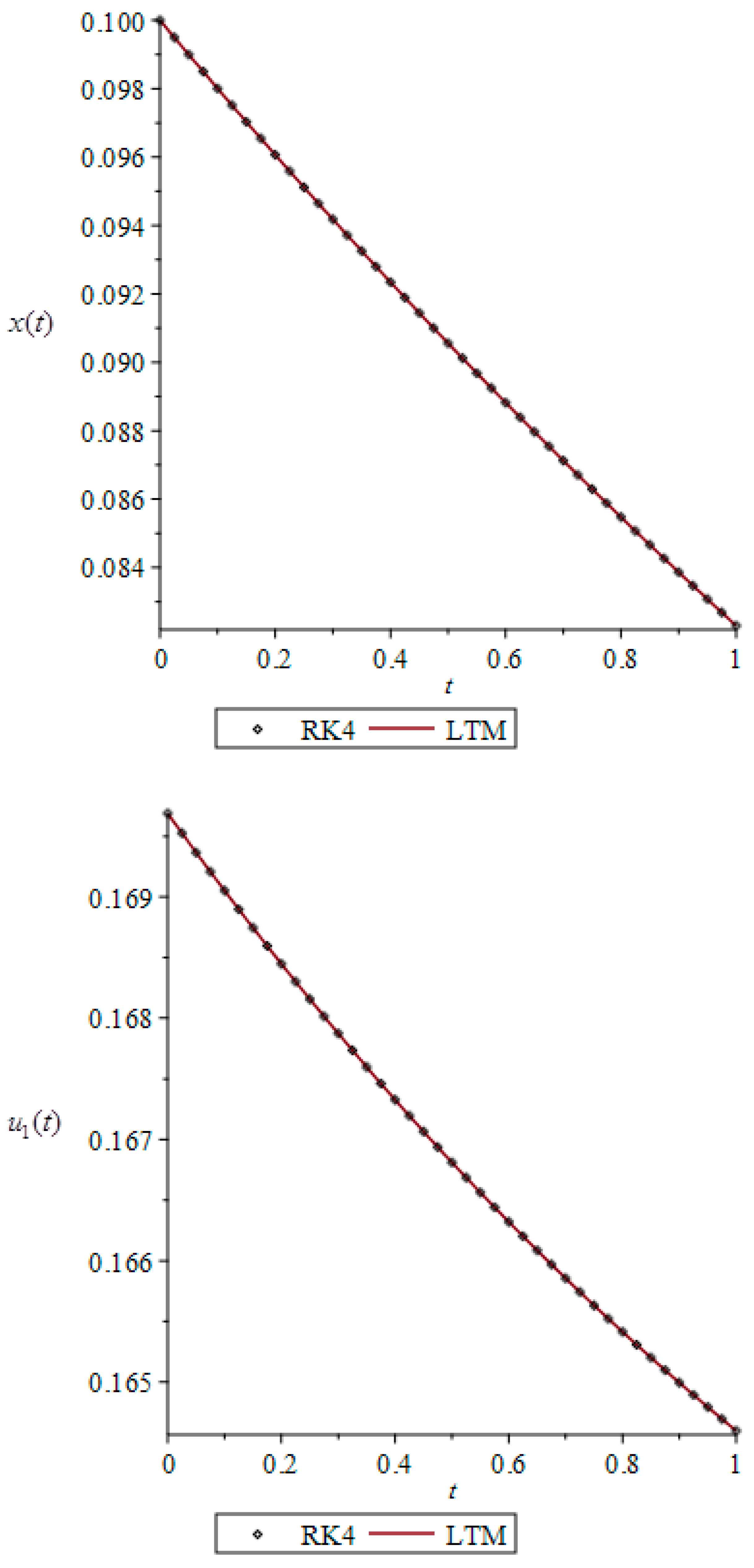
The numerical results for optimal payoff functionals $J_1$ and $J_2$ with different values of $N$ are shown in

Table 1. Optimal payoff functionals $J_1$ and $J_2$ for illustrative example with LTM as compared with RK4.

$\mathit{N}$	${\mathit{J}}_{1\mathit{L}\mathit{T}\mathit{M}}$	${\mathit{J}}_{2\mathit{L}\mathit{T}\mathit{M}}$
8	0.016380209069964074615873141557194	0.0092479570969023022143164502992464
10	0.016380209069964074615873178289759	0.0092479570969023022143164746205906
12	0.016380209069964074615873178289820	0.0092479570969023022143164746206322
14	0.016380209069964074615873178289819	0.0092479570969023022143164746206318
$\Delta t$	$J_{1RK4}$	$J_{2RK4}$
${10}^{-4}$	0.016380209069970129334132078913143	0.0092479570969076035409551440677725

and compared with RK4. The graphs of approximate solutions for open-loop Nash equilibrium for $N=14$ are given in Figure 1.

5. Conclusions

This paper has dealt with the numerical solution for obtaining the open-loop Nash equilibrium of nonlinear nonzero-sum differential games in a finite horizon based on the Legendre Tau method (LTM). Regarding this method, the solution functions of the system of TPBVPs derived from Pontryagin’s maximum principle were expanded in terms of Legendre polynomials and then a system of algebraic equations was obtained. A differential game arising from a bioeconomic model was considered to demonstrate the accuracy and efficiency of the proposed method. A comparative study between the presented method and the fourth order Runge–Kutta method (RK4) was presented graphically.