Article

Generating Trees for Comparison

Faculty of Electrical Engineering and Computing, University of Zagreb, Unska 3, 10000 Zagreb, Croatia
*
Author to whom correspondence should be addressed.
Computers 2020, 9(2), 35; https://doi.org/10.3390/computers9020035
Submission received: 28 February 2020 / Revised: 22 April 2020 / Accepted: 24 April 2020 / Published: 29 April 2020

Abstract

:
Tree comparisons are used in various areas with various statistical or dissimilarity measures. Given that data in various domains are diverse, and a particular comparison approach could be more appropriate for specific applications, there is a need to evaluate different comparison approaches. As gathering real data is often an extensive task, using generated trees provides a faster evaluation of the proposed solutions. This paper presents three algorithms for generating random trees: parametrized by tree size, shape based on the node distribution and the amount of difference between generated trees. The motivation for the algorithms came from unordered trees that are created from class hierarchies in object-oriented programs. The presented algorithms are evaluated by statistical and dissimilarity measures to observe stability, behavior, and impact on node distribution. The results in the case of dissimilarity measures evaluation show that the algorithms are suitable for tree comparison.

1. Introduction

Trees as data structures are used to represent hierarchically organized data in various areas, such as pattern recognition [1,2], phylogenetic studies [3], structured documents [4], and problem-solving by searching [5]. In the mentioned areas, one of the key tasks is to compare trees, e.g., by tree characteristics and dissimilarity measures. Tree characteristics such as tree height and node degree, and conclusions based on these characteristics, such as branching factor [5], can provide insight into the relationships in the data. In order to determine how similar two data patterns represented by trees are, dissimilarity measures are introduced [6], such as tree inheritance distance (TID) from our previous work [7]. Dissimilarity measures are related to the problem domain; e.g., dissimilarity measures used in computer vision rely on the structural differences between ordered trees. When there is a need to use or to introduce dissimilarity measures specific to the problem domain, it is useful to compare various trees by the results from the dissimilarity measures. The data used to evaluate various approaches can be extracted from real-world cases or generated. Real data is the basis for problem-solving from a specific domain. However, gathering real data is often an extensive task, whereas data generated by a random tree or a tree similar to the tree created from real data provides a faster evaluation of the proposed problem solutions.
In this paper, we briefly describe tree comparison based on the dissimilarity measures and tree characteristics such as height and degree, followed by the elaboration of trees’ statistical data relevant for use in the presented algorithms. The contributions of this paper are three algorithms for generating unordered trees: random, using a given node distribution corresponding to the data in the problem domain, and trees created by the modification of the existing tree. Our primary motivation is to generate trees representing the class hierarchy in object-oriented languages. As an example, to create a tree that reflects real data from a problem domain, a distribution pattern is obtained from several open-source programs to form parameters. However, the presented algorithms can also be used in other problem domains. Besides, a web tool for generating trees is developed based on the presented algorithms (see Appendix A for more information).
The remainder of the paper is organized as follows. In Section 2, as the preliminaries, statistical and dissimilarity measures are briefly described and presented in the context of the class hierarchy of an object-oriented program. In Section 3, tree algorithms to generate trees, with emphasis on the tree comparison, are introduced. Furthermore, the evaluation of presented algorithms is performed by analyzing the results of the experiments in Section 4. The last section is the conclusion.

2. Preliminaries

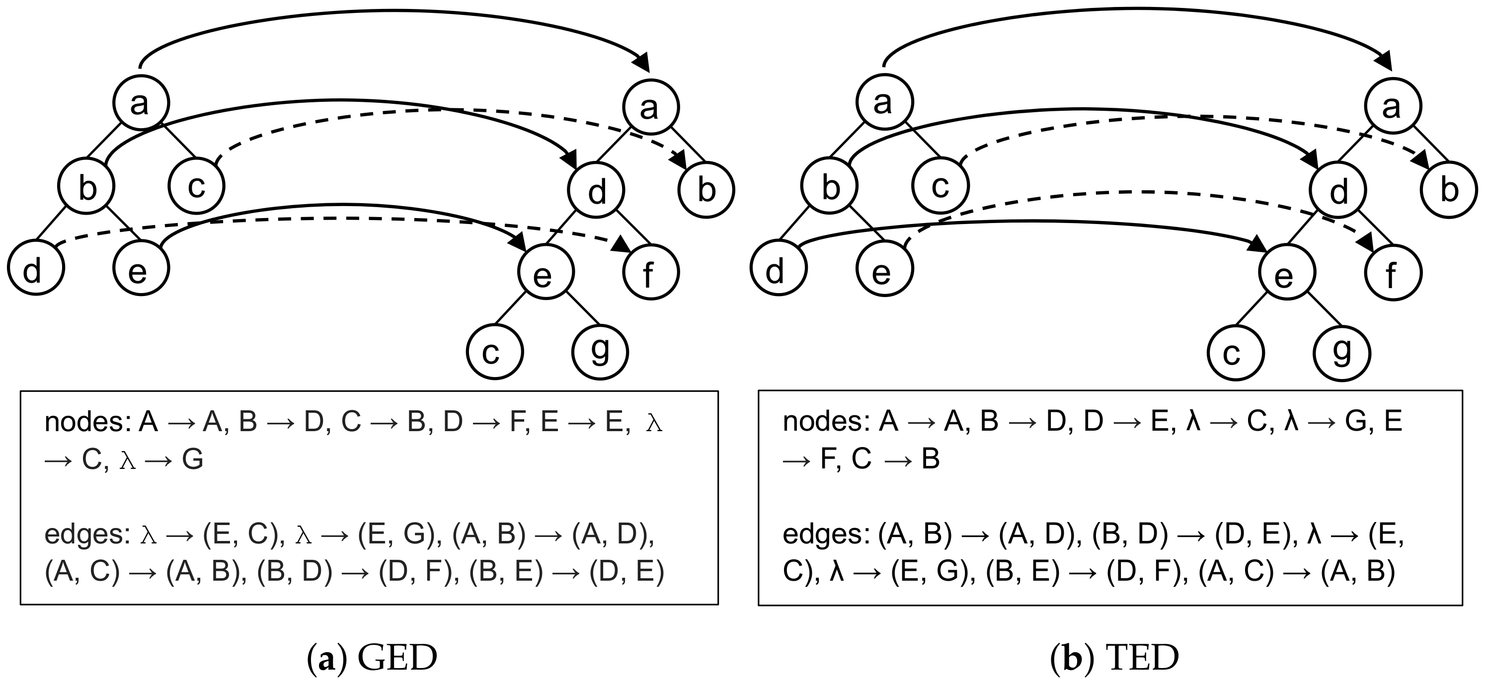
2.1. Dissimilarity Measures

The dissimilarity value is a single number that represents the difference between trees and graphs [8,9,10]. There are various dissimilarity measures; however, in this paper, we use edit distance since it provides "error-tolerant" matching of trees [11], because compared trees can be entirely dissimilar. Edit distance is calculated by operations applied to nodes and edges of a tree, such as add, delete, and substitute. Each operation is assigned a cost, where edit distance is the minimal cost of operations to transform a tree from one to another. There are various algorithms and constraints to calculate edit distance, based on the type of the tree or problem domain; e.g., TED—tree edit distance is used on ordered trees where add and delete operations are performed only on leaf nodes [6], whereas GED—graph edit distance is suitable for graphs, and used in pattern recognition [11]. E.g., GED in [11] uses a best-first algorithm (A*) to calculate the minimum distance in result space over all possible operation combinations. Since edit distance depends on the constraints and the algorithm being implemented, edit distances differ in the result and operation set or sequence; e.g., Figure 1 shows nodes mapping between two trees as the results of the GED and TED algorithms. The GED value in Figure 1a is equal to seven, while the TED value in Figure 1b is equal to six. The GED includes the cost of both node and edge operations, whereas in TED, the cost of edge operations is implicitly included in the cost of operations performed on nodes. Specified distance values are valid when the costs for add, delete, and substitute operations are equal to 1, and in the case of the GED, add and delete edge operations. On Figure 1 nodes and edge operations are shown in squares, where λ represents empty node and edge, such that, e.g., λ c denotes add node operation. Moreover, if nodes b and d as children of the root node change order, GED value will remain unchanged, whereas the TED value, in that case, is equal to 7. There is an additional add node operation λ b and instead of operation c b operation c λ is performed. The difference is a consequence of the fact that the TED algorithm is used for ordered trees, whereas the GED algorithm is used for unordered trees. These two algorithms are selected to show how various algorithms result in different distance values, which is discussed as the result of the experiments in Section 4.

2.2. Statistical Measures

Tree characteristics such as the number of nodes (n), height (h), and the level and degree of nodes are used to analyze the shape of a tree. Statistical values based on those measures involve a number of nodes for each level; i.e., the number of nodes per level— N l and average nodes degree per level D a . The number of nodes per level is a sequence N l = ( n 1 , , n i , , n m ) , where the n i denotes number of nodes in the tree at the level i. Average node degree per level, i.e., average number of children per level, is a sequence D a = ( d 1 , , d i , , d n ) , where d i is the average degree at level i. N l provides information about the distribution of nodes at each level, while D a provides insight into average branching at each level. Note that the D a is similar to the average branching factor used in the domain of solving problems by searching [5], where the emphasis is on the branching factor of the entire tree or algorithm iteration. However, in this paper, D a is based on the node level. Both N l and D a provides information about the shape of the tree.
Table 1 shows statistics based on the class hierarchy of an open-source program NewPipe [12] for program versions 0.8.9 and 0.9.0. The data in Table 1 show that version 0.9.0 in comparison to the 0.8.9 contains fewer nodes (n); it is shallower (h), but the distribution is relatively stable, since nodes are mostly contained in the first two levels ( N l ); and it has a similar branching at the level 2, with a tendency of reducing the number of nodes at higher levels.
Moreover, Figure 2a shows how the distribution of nodes per level N l is similar between trees of NewPipe class hierarchy for 10 subsequent program versions from 0.8.8 to 0.9.12. The average number of nodes per level for all currently available 62 NewPipe [12] versions is represented by the blue line in Figure 2a. The distribution shape for 10 subsequent version corresponds to the node distribution in 62 versions. In order to get a more precise approximation of tree shape and node distribution, besides NewPipe, another four programs with publicly available source code were analyzed and the average node distribution is shown in Figure 2b. Average values show a similar tendency on the same levels between different programs and correspond to the values shown in Figure 2a. Both figures show a pattern for class hierarchy in the form of a node distribution.

3. Generating Trees

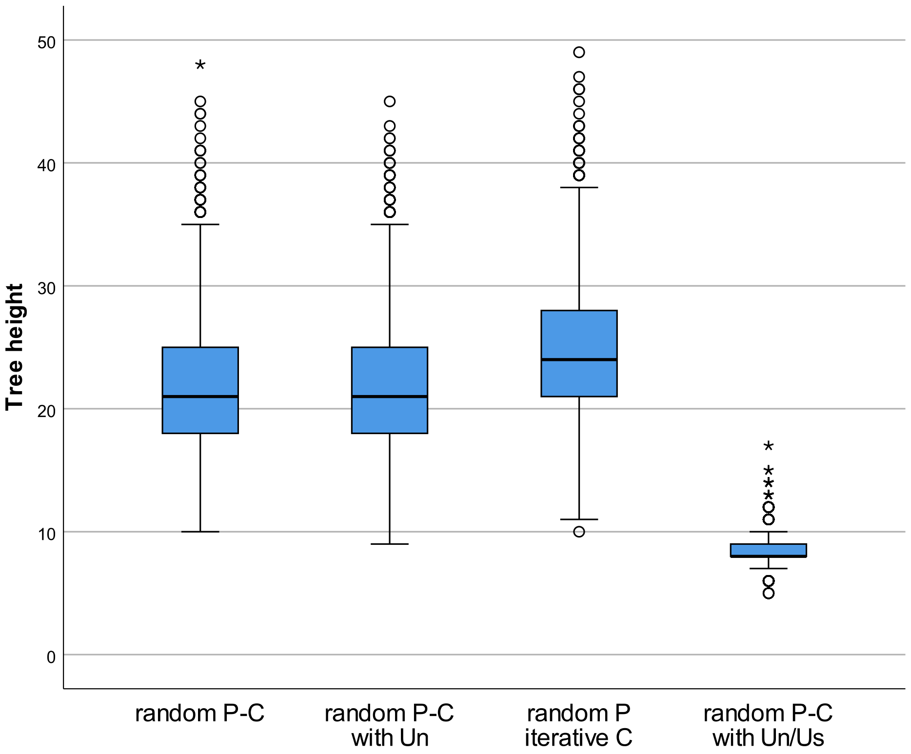
3.1. Random Variants

A simple approach to generate a single tree is by randomly creating a given number of nodes and edges. In this paper, to generate trees randomly, we rely on a pseudo-random generator. The algorithm to generate a tree by randomly selecting nodes to connect is shown in Algorithm 1. The presented algorithm is generic, where variants of the algorithm are shown using Table 2. The algorithm variant is obtained from generic Algorithm 1 by replacing the keywords denoted with square brackets with the corresponding values in Table 2. The algorithm accepts the number of nodes n as input, and the output is a set of nodes V and a set of edges E. The algorithm first creates n nodes, and then selects parent ([parent]) and child ([child]) nodes to connect based on the condition ([condition]) until there is n 1 edges. Algorithm variants differ in use of an additional node sets which are initialized ([initialize]) before connecting the nodes and adjusted ([adjust]) after the pair of nodes is connected. Function newNode creates a new node, whereas newEdge returns an edge consisting of two nodes, the parent and child nodes. Function getRandomNode from Table 2 randomly selects a node from the given set of nodes, whereas getNextNode returns nodes consecutively. Function getPreds traverse tree from the given node to the root node returning the predecessor node-set.
Algorithm 1: Random tree algorithm
  input:  the number of nodes n.
  output:  Tree T ( V , E )
1
V , E ;
2
for i 1 to n by 1 do
3
   V V { newNode ( ) } ;
4
end
5
 [initialize];
6
do
7
   u p [parent];
8
   u c [child];
9
  if [condition] then
10
    E E newEdge ( u p , u c );
11
   [adjust];
12
  end
13
while | E | < n 1 ;
There are four variants of algorithm, depending on the parent and child selection, random or consecutive, and depending on the sets of nodes from which the nodes are selected (Table 2). Various variants are considered in order to determine how variants with different time and space complexities affect generating different trees. The algorithm variant with random parent and child node selection from node-set V (random P-C) contains a condition given in Table 2 to avoid cycles. However, this variant performs traversal of both u c and u p nodes to the root node by function getPreds to obtain predecessor nodes, increasing the time complexity. Traversal complexity is equal to O ( k ) , where k represents the average node level in the tree. In order to discuss the time complexity of the given algorithm only, a particular random function complexity (getRandomNode) and a function for retrieving consecutive nodes (getNextNode) are not considered. Therefore, it is assumed that both functions have complexity O ( 1 ) . Algorithm time complexity is O ( n k ) , besides random P-C with U s / U n variant with time complexity O ( n ) . The Algorithm 1 variant with random parent and child node selection from the node-set V and unused set U n (random P-C with U n ) use additional space to store nodes without a parent node. Therefore, only predecessor nodes for node u p are retrieved. Another algorithm variant (random P iterative C) is with a random selection of parent node only, where child nodes are iteratively selected. The stated algorithm variants require the condition whether the selected child and parent nodes are equal (Algorithm 1 line 9), which can increase the number of attempts to select a different parent and child. Therefore, another algorithm variant (random P-C with U s / U n ) is evaluated with used ( U s ) and unused ( U n ) sets of nodes. The unused set is equal to the node set U n in variant random P-C with U n , containing nodes without a parent, whereas a set of nodes U s contains nodes with the already added parent. Using two disjunct sets of nodes avoids checking that the randomly selected parent and child are the same node. Since various algorithm variants to create connections could randomly be incorporated, some algorithms tend to expand horizontally and others vertically. A desirable random tree algorithm is the one that can generate both wide and deep trees randomly between different runs. Algorithm variants are empirically evaluated by generating 10,000 trees with 100 nodes. Figure 3 shows a box plot for the height of trees generated by Algorithm 1 variants. The first three variants generate trees with a similar range of heights, whereas random P-C with U s / U n generates shallow and wider trees. A wider tree is the result of connecting nodes in order from the root node, where each step of the algorithm creates a valid tree. Furthermore, random P iterative C algorithm variant generates deeper trees, but the first two algorithm variants generate trees with a slightly better height variation (Figure 3). A similar conclusion can be drawn from the average tree height values in Table 3. In addition, Table 3 contains an average number of selected equal parent and child nodes corresponding to equal hits (EH) for each variant in Table 3. It can be concluded that random P-C with U n variant provides a good variation of tree height shown in Figure 3, with smaller EH values (Table 3) and less time complexity. In the experiments in Section 4, variant random P-C with U n is used as Algorithm 1 for the algorithm evaluation.

3.2. Generating Trees by Node Distribution

The tree generated by Algorithm 1 is shown in Figure 4, represented by the radial visual layout (twopi) [13]. Figure 4 shows how tree branching is scattered, corresponding to random connections between nodes, which is also confirmed by node distribution per level on Figure 5 denoted as alg1. Algorithm 1 is suitable for scenarios where a random connection between nodes is required. However, domain data usually follows certain patterns; e.g., a distribution of nodes per level for the class hierarchy of NewPipe in versions 0.8.9 and 0.9.0 is shown in Figure 5. The shown pattern reflects that the nodes are mostly concentrated on the first two levels. At higher levels, the concentration of the nodes decreases. In order to generate a tree that reflects real data from a particular domain or observed phenomenon, another approach is required, based on the distribution pattern obtained from the real data. Therefore, we introduce Algorithm 2 to generate a tree based on the given distribution of nodes per level. Connections between nodes are generated randomly, where nodes at current level are randomly selected from a set of nodes without parent node—N, and are connected to a randomly selected node from a set of nodes at the previous level—P. The algorithm creates a tree level by level: first, the root node is randomly selected—r, and then nodes for each level—u. The number of nodes at each level (C) is determined by function getNodeCountPerLevel based on the given distribution of nodes in percentage—D, number of nodes—n, and current level i. Finally, a set of nodes in the current step in algorithm—T becomes a set of predecessor nodes—P in the next step.
Instead of the given distribution of nodes, a random distribution can be used in Algorithm 2. The getNodeCountPerLevel function can return a random number of nodes per level for a given level, resulting in distribution of nodes, as shown in Figure 5, for the tree height of 5 as alg2-rand-dist. In addition to the random node distribution, the number of levels could also be randomly determined, e.g., in pre-defined intervals to achieve randomization both of node distribution and tree height.
Algorithm 2: Random tree by node distribution.
  input: the number of nodes n and node distribution per level D (expressed as percentages)
  output: Tree T ( V , E )
1
V , E ;
2
for i 1 to n by 1 do
3
   V V { newNode ( ) } ;
4
end
5
N V ;
6
u r getRandomNode (N);
7
N N { u r } ;
8
P { u r } ;
9
for i 1 to | D | by 1 do
10
   T ;
11
   C getNodeCountPerLevel (D, n, i);
12
  for j 1 to C by 1 do
13
    u c E getRandomNode (N);
14
    u p getRandomNode (P);
15
    E E newEdge ( u p , u c );
16
    N N { u c } ;
17
    T T { u c } ;
18
  end
19
   P T ;
20
end

3.3. Distorted Tree

The first two algorithms generate random trees by the given number of nodes and distribution of nodes. In order to compare two trees, one of the possibilities is to generate two independent trees using these algorithms. However, it is unlikely that two unrelated trees would be compared. In the case of the class hierarchy, a comparison is performed between two versions of the program. Therefore, it is necessary to modify the original tree to obtain another tree for comparison; e.g., to evaluate dissimilarity measures described in Section 2. The difference between created trees can be controlled by distortion parameters as the amount of added, deleted, and matched nodes with the changed parent, similarly to operations performed on nodes in edit distance algorithms. Moreover, by changing the specific distortion parameter, tree dissimilarity measures can be evaluated, and tree statistics analyzed. Generally, parameters can be used in domains where the controlled difference between generated trees for comparison is required; e.g., a domain where the tree can differ in only added or deleted nodes. The algorithm to generate trees based on the given tree and the amount of distortion is given in Algorithm 3.
Algorithm 3: Tree generated by given source tree and distortion parameters.
  input:  Tree T 1 ( V 1 , E 1 ) , distortion parameters a, d, m p
  output:  Tree T 2 ( V 2 , E 2 )
1
V 2 V 1 , E 2 E 1 ;
2
for i 1 to d by 1 do
3
   u d getRandomNode ( V 2 );
4
   V 2 V 2 { u d } ;
5
   E 2 E 2 getEdgeToParent ( u d );
6
  if hasChildren ( u d ) then
7
    u p getParent ( u d );
8
   foreach c in getChildren ( u d ) do
9
     E 2 E 2 {getEdgeToParent (c)};
10
     E 2 E 2 {newEdge ( u p , c)};
11
   end
12
  end
13
end
14
M V 2 ;
15
for i 1 to a by 1 do
16
   u a newNode ();
17
   u p getRandomNode ( V 2 );
18
   V 2 V 2 { u a } ;
19
  if hasChildren ( u p ) ∧ spreadDecision () then
20
    c getRandomChild ( u p );
21
    E 2 E 2 {getEdgeToParent (c)};
22
    E 2 E 2 {newEdge ( u a , c)};
23
  end
24
   E 2 E 2 {newEdge ( u p , u a )};
25
end
26
m c m p | M | ;
27
N M ;
28
for i 1 to m c by 1 do
29
   u m getRandomNode (N);
30
   u o p getParent ( u m );
31
   u n p getParent ( V 2 { u m , u o p } );
32
   E 2 E 2 {getEdgeToParent ( u m )};
33
  if hasChildren ( u n p ) ∧ spreadDecision () then
34
    c getRandomChild ( u n p );
35
    E 2 E 2 {getEdgeToParent (c)};
36
    E 2 E 2 { newEdge ( u m , c)};
37
  end
38
   E 2 E 2 {newEdge ( u n p , u m )};
39
   N N { u m } ;
40
end
Algorithm 3 accepts source tree ( T 1 ) and distortion parameters to create a target tree ( T 2 ) as the number of added (a) and deleted nodes (d), and percentage of matched nodes with changed parent ( m p ). Matched nodes are nodes with the same labels in both source and target tree. The algorithm works as follows: first, nodes V 1 and edges E 1 of the source tree are copied into V 2 and E 2 . Matched nodes are stored in set M, corresponding to the set V 2 after the node deletion. The algorithm randomly selects d nodes from set V 2 by using function getRandomNode. Randomly selected node u d is deleted from set V 2 , together with the corresponding edge to the parent node from the set of edges E 2 . The edge that is deleted is obtained by function getEdgeToParent and given the child node. Upon deletion, the algorithm creates new nodes and adds them to the node-set V 2 . For each new node u a the algorithm randomly selects its parent node u p and creates a corresponding edge ( u p , u a ) . If the parent node has children, the tree can be additionally modified by replacing the parent of one of the randomly selected children c and set u a as the new parent. This modification depends on the spreadDecision function, which in this paper decides with a 50% chance. However, the function can be parametrized or defined differently based on specific usage. The third step of the algorithm is to replace parent node for matched nodes from set M. First, the number of parent-changing nodes m c is calculated over the parameter m p and the number of matched nodes | M | . Node u m is selected from a set of nodes N, which initially contains matched nodes M. At each iteration performed m c times, set N is reduced by node u m . The algorithm acts similarly for adding the nodes; it randomly selects a new parent node u n p from a set of nodes V 2 { u m , u o p } , where a newly added node, as a matched node, can be the new parent node. Similarly to the adding node, node u m can be added as child to the new parent u n p in two ways: by replacing the existing child node c or adding it as the new child node. The difference is that the edge ( u o p , u m ) to the previous parent node u o p is deleted from set E 2 . On the other hand, the final number of nodes with a changed parent may eventually be greater than M. Deleting a node with children involves changing the parent of the child, and in cases where a new or an existing node replaces the child, that child changes the parent. However, in this paper, we consider such changes implicitly with the initial distortion parameters. Future work could include an evaluation of Algorithm 3 that would consider such changes separately. Algorithm 3’s complexity is in the worst-case O ( n 1 + n 2 ) when n 1 nodes are deleted, and n 2 nodes are added, where n 1 corresponds to d, and n 2 corresponding to a. An example of tree generated by Algorithm 3 from the tree shown in Figure 6a as the source tree with 100 nodes is shown in Figure 6b. The distortion parameters used are 10 added and deleted nodes and 10% of matched nodes with changed parents (10, 10, 0.1). Note that tree in Figure 6a is generated by Algorithm 2 with the following distribution: 32.5%, 50%, 10%, 5%, and 2.5%. The given distribution of nodes corresponds to the distribution of tree representing class hierarchy of NewPipe program version 0.8.9 shown in Figure 5. Trees in Figure 6a,b are similar, since the tree in Figure 6b is generated by controllable distortion of source tree in Figure 6a. On the other hand, the tree in Figure 6c is generated by Algorithm 2 with the same distribution as the tree in Figure 6a. An approach where both trees are generated by Algorithm 2 can also be used to generate trees for comparison. In this case, the distribution of nodes in both trees is equal, but the distortion is in the form of a possibly different number of nodes and random connections between nodes.

4. Experiments

Experiments evaluate algorithms proposed in the previous section by the effect of the variation in the statistical and dissimilarity measures of generated trees. The effect is observed by changing the distortion parameters and node distribution. In the first experiment, the source tree generated by Algorithm 1 and target tree generated by Algorithm 3 are analyzed to show the stability of the algorithms. The analysis is performed by using the N l and D a statistical measures, and GED and TED edit distances described in Section 2. Stability is evaluated by whether the algorithms will generate relatively similar trees between different runs with the same parameters. In the second experiment, the change in edit distance is analyzed by changing the distortion parameters. TED is calculated between the source tree generated by Algorithm 1 and target distorted tree generated by Algorithm 3. Through the experiment, we want to gain insight into the behavior of the Algorithm 3 when applied to the random tree generated by Algorithm 1. The influence of a single distortion parameter is analyzed by the difference between trees in the form of the TED algorithm and operations. In the third experiment, the source tree is generated by Algorithm 2 and the target tree by Algorithm 3. By the third experiment, changes in node distribution between the source and the target tree are analyzed to observe how the distribution is affected by the distortion when it is necessary to compare trees from various domains represented by a corresponding node distribution pattern. In the experiments, the cost for all edit distance operations is set to 1, where substitute operation has a cost of 1 if the labels of the nodes differ. The results of the experiments were obtained using a software tool developed using the algorithms described in Section 3 (see Appendix A for the source code).

4.1. Statistical and Edit Distance Measurements

In the experiment, the generated source tree is distorted to obtain a target tree for ten consecutive comparisons of the source and target tree by statistical and dissimilarity measures. Both the source and target trees are the size of 10 nodes because the time complexity for the used GED best-first algorithm (A*) without heuristics grows exponentially with the number of nodes [11]. To generate a source tree, number 10 is used as an input parameter for the Algorithm 1, whereas to generate the target tree, the source tree and distortion parameters (1, 1, 0.5) are used as input parameters for Algorithm 3. The generated source tree is a random tree with 10 nodes, and the target tree is the source tree with one deleted node, one added node, and four nodes with the changed parents. Between the source and target tree, eight nodes are matched, where 50% of these nodes correspond to four nodes with the changed parent. Since add and delete operations in TED are performed on the leaf nodes only, the number of TED operations is higher than the number of GED operations, it is expected that the TED values will be higher than the GED values.
The results of ten consecutive executions of Algorithms 1 and 3 are shown in Table 4. The last row contains the average results of 30 runs. Results for N l 1 in Table 4 show that Algorithm 1 generated trees of 10 nodes with height from 4 to 8, while N l 2 shows that height for trees generated by Algorithm 3 is on average smaller. In Algorithm 3, nodes are randomly selected between all nodes in the tree with equal probability. In the case of adding a node and changing node parent, there is a higher chance of adding a node at lower levels, increasing the tree in width and decreasing the height of the tree. Deleting a node can also cause a decrease in tree height, as children of a deleted node move to the previous level. Average degree per level D a 1 corresponds to the ratio between the number of nodes at the next and current level. Moreover, Table 4 shows as expected smaller values for GED than TED. Average and standard deviation values indicate that the distance values between generated trees for both GED and TED are stable between runs. The results of distance values are related to the number of nodes in the tree, which means that the number of nodes limits the number of edit operations. We can also conclude that the algorithms for generating trees are stable because, for the same parameters and distortion between trees, the algorithms generate on average trees with relatively similar edit distances.

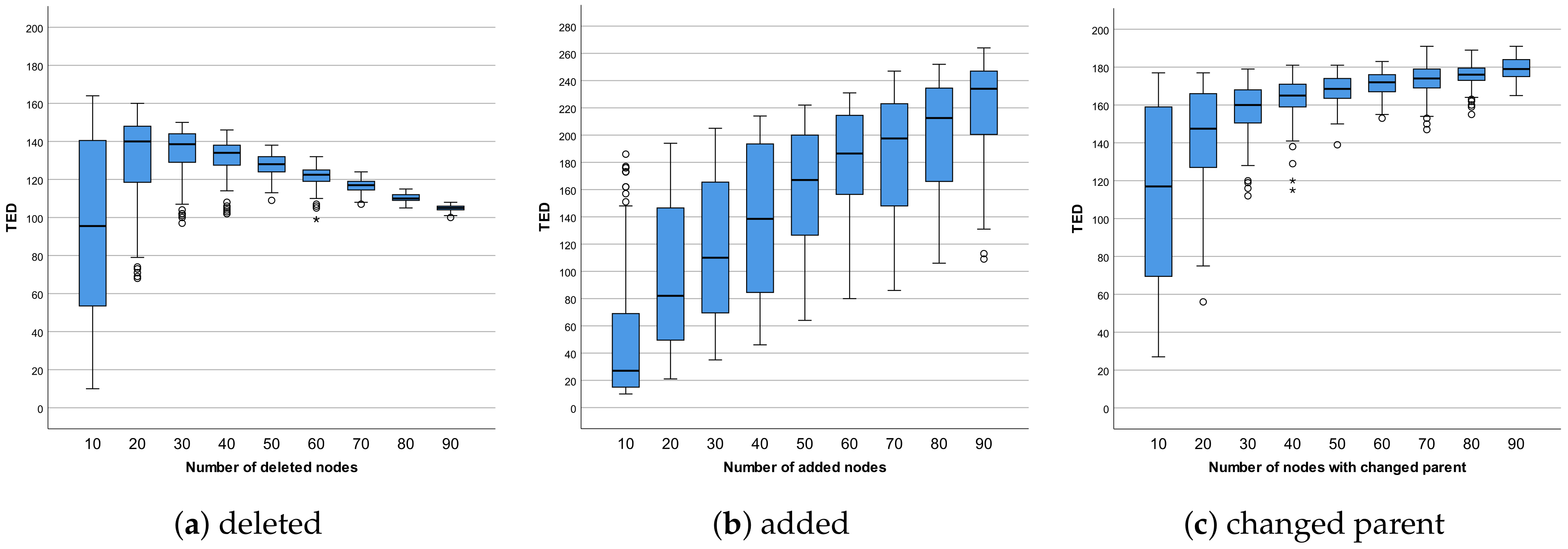
4.2. Distortion Parameters

The experiment consists of three experimental setups in which the source tree generated by Algorithm 1 is compared with the target tree obtained by Algorithm 3, to show the effect of the single distortion parameter of the Algorithm 3 separately on the source tree change. Unlike the first experiment, the source tree is the size of 100 nodes; therefore, to calculate edit distance in a reasonable time, we use the TED algorithm only. In the first experimental setup, the number of deleted nodes incrementally increases from the initial 10 (10, 0, 0) to the final 90 nodes (90, 0, 0) in increments of 10 nodes. Similarly, in the second experimental setup, instead of deleted nodes, the number of added nodes increases. In the third experimental setup, the percentage of matched nodes between the source and target trees, that change the parent, incrementally increases from the initial 10% (0, 0, 0.1) to the final 90% (0, 0, 0.9) in increments of 10%. Since there are no added or deleted nodes, the source and target tree contain the same node-set of 100 nodes, therefore all nodes are matched, and the number of nodes with changed parent incrementally increases from the initial 10 to the final 90 nodes in increments of 10 nodes. As the number of nodes involved in changes increases, the number of operations is expected to increase. Considering the expected increase in the number of operations and the cost of operations is equal to 1, the resulting edit distance is also expected to increase. For each experimental setup separately, source and target trees were generated 100 times and compared using the TED algorithm. The results of the experiment are shown as the distribution of TED values obtained during the comparisons in the form of box-whisker graphs shown in Figure 7.
The results of the first experimental setup are shown in Figure 7a. A variation of the edit distance value, observed as the interquartile range in the box-whisker graph, decreases with the number of deleted nodes. Edit distance, observed as the median value, increases with the increased number of deleted nodes but decreases after 40 deleted nodes. An increase and then decrease of distance are related to the used distance algorithm and the number of deleted nodes. Deletion of a smaller number of random nodes in the source tree results in variations of possible add, delete, and substitute TED operations. The consequence is a considerable variation of distance. Moreover, as the number of deleted nodes slightly increases, there is an increase in the number of operations. However, when the number of deleted nodes is significant compared to the total number of nodes in the source tree, the distance decreases because delete operations prevail. For the same reason, there is a decrease in variation. In that case, edit distance is mostly calculated based on the cost of delete operations. Furthermore, as there is an unchanged number of deleted nodes between different runs, edit distances are similar, resulting in smaller variations.
The results of the second experimental setup, where the number of added nodes is increasing, are shown in Figure 7b. As expected, the distance increases with the increasing number of added nodes. Since the number of added nodes increases, the number of operations increases, and therefore the total transformation cost. On the other hand, the change in distance variation is not constant as the number of added nodes increases because Algorithm 3 can add a new node as a child node of the existing or previously added nodes, resulting in different edit distance values.
Figure 7c shows the results of the third experimental setup, where matched nodes change the parent node. An increase in distance with the increased percentage of changes is as expected, similar to the setup with adding nodes. However, the increase in distance slows as the number of nodes with the changed parent increases. As the number of nodes with changed parent increases, the total number of nodes does not change, which limits the possible number of operations and, as a consequence, the value of edit distance. On the other hand, the number of add and delete operations increases, with the increasing number of randomly selected nodes with changed parent. However, variation decreases with an increasing percentage of involved nodes, similar to delete setup. Furthermore, a large number of nodes involved in operations results in similar distances between different runs.
Experiment results show that in the case of the add and parent change distortion parameters, trees are more dissimilar, as parameters increase. A relatively large variation in the case of add node parameter is the consequence of the Algorithm 3 random placement of the inserted node. Although Algorithm 3 for the parent change parameter, similar to the add parameter, randomly relocates nodes in the tree, there is a decrease in the variation as a consequence of the unchanged number of nodes. On the other hand, distance decreases in the case of the delete parameter, which is related to the smaller number of affected nodes in operations and used TED algorithm.

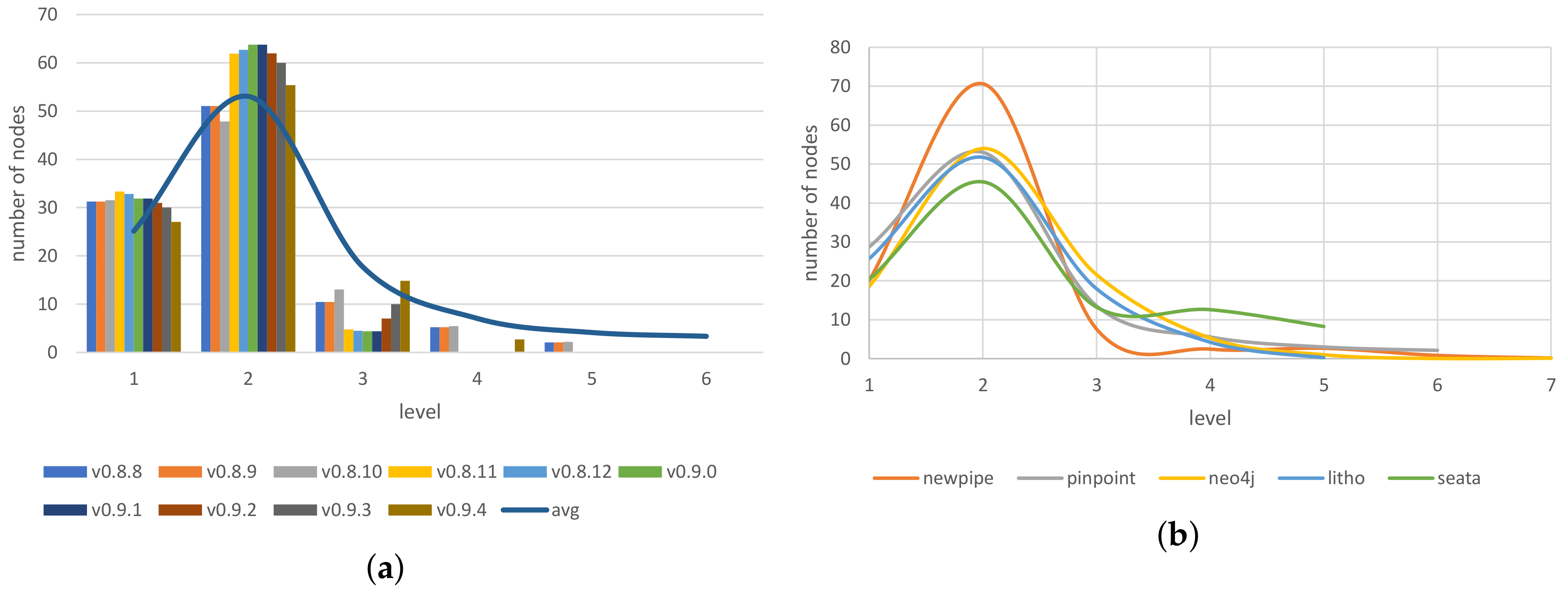
4.3. Node Distribution

Since the experiment analyzes the influence of distortion parameters on the distribution of nodes by level, the source tree is generated by Algorithm 2 to generate a tree with initial node distribution, and a target tree is generated by Algorithm 3 to distort the source tree and analyze resulting node distribution in the target tree. Similarly to the second experiment, various combinations of distortion parameters of Algorithm 3 are used, with only added (50, 0, 0), deleted (0, 50, 0), and nodes with the changed parent (0, 0, 0.5). Furthermore, to analyze the influence of a single distortion parameter on the changes in the node distribution, the results of a single parameter are compared with the result of the combined distortion parameters (10, 10, 0.1).
Besides the node distribution pattern detected in Section 2.2 for class hierarchy of object-oriented languages, different node distributions are possible, depending on the problem domain. Therefore, in the experiment, various initial distribution of nodes are used to analyze changes in the distribution for various possible domains. In Table 5 column T 1 Input Distribution contains input distribution to generate the source tree, and column T 1 Output, node distribution of the generated source tree as a spark-line graph. The first row contains the source tree generated by the node distribution corresponding to the average node distribution of NewPipe class hierarchy in available versions shown in Figure 2a and the rest of the rows contain source trees generated by various node distributions. Furthermore, Table 5, from columns 3 to 6 ( T 2 Output by Distortion Parameters), contains the node distribution in the target tree for various distortion parameters to observe the effect of the distortion parameters on the node distribution in the target trees. Node distribution in target trees is shown as a spark-line graph of the average node distribution in the target tree, calculated from the experiment results obtained by 100 runs. Markers on spark-line correspond to the node distribution at a particular level. For analysis of the experiment results, spark-line graphs of the source and target trees are compared.
The results in Table 5 show that the distribution of nodes in the target tree, generated by adding 50 nodes to the source tree (50, 0, 0), closely follows the distribution of nodes in the source tree, up to the level of the height of the source tree. At levels higher than the height of the source tree, the number of nodes in the target tree decreases. The height of the target tree can increase in a couple of cases. In the case when the leaf node at the height of a tree is selected as the parent for the new node, tree height increases. The same applies when the non-leaf node is selected because when the new node is inserted as a child instead of the existing child, children move to the next level. Consequently, the number of nodes at the next level increases with a possible decrease in the previous level. On the other hand, if a new node is added as the new child of the selected parent, the number of nodes at the children’s level increases without increasing the tree height. Therefore, the target tree increases in height, and possibly in the number of nodes at the particular levels. Such behavior of Algorithm 3 is visible by the node distribution among the source trees with different node distributions, but mostly on the source tree with the even distribution of nodes. Similar behavior of the algorithm is in the case when 50 nodes change the parent node (0, 0, 0.5). Then, the algorithm randomly selects another parent for matching nodes, where a node can be inserted instead of the existing children or added as a new child. Contrary to the case of adding nodes, the effect of a decreased number of nodes at higher levels is more pronounced since the total number of nodes remains equal. On the other hand, observed through the node distribution, for delete distortion parameter (0, 50, 0) target tree, the number of levels decreases because children of deleted nodes move to the previous level. For the same reason, the number of nodes with higher levels decreases resulting in falling node distribution.
Furthermore, in the case of the half-rounded distribution, there is a visible effect of variation in the number of nodes at the end of the tree in a sinusoidal form. A similar effect is observable in the case of deleting nodes, which is a consequence of moving child nodes between levels. The detected variation effect is also visible in a tree with 10 levels and even distribution, and since in the case of half-rounded distribution, the tree is of 13 levels, it can be concluded that for a source tree of greater height, the effect of the variation will be higher. On the other hand, results in the case of the combined parameters (10, 10, 0.1) with 10 added, deleted, and nodes with the changed parent show that all three single parameters influence the target distribution. However, the target distribution is mostly influenced by the change of the parents’ distortion parameter, since the resulting spark-line is most similar to the spark-line in the case of the parents change.

5. Related Work

Random trees from the related literature do not apply to the case of the class hierarchy in object-oriented languages. Random trees are usually generated from the root node [14], whereas Algorithm 1 variants, besides random P-C with U n / U s create trees by selecting nodes without a parent. Recursive tree [14] is created by connecting a new node to the randomly selected node in the previously added set of nodes, starting with the root node. The process of generating tree in the Algorithm 1 variant random P-C with U n / U s corresponds to the generating recursive trees. However, unlike trees generated by algorithms presented in this paper, recursive trees are labeled with distinct integer numbers, which incrementally increase starting from the root node labeled with the number 1, which is not feasible for scenarios with arbitrary labels. Furthermore, random binary tree [15,16] can be created in two ways by randomly inserting nodes, one by one or by randomly selecting one tree from all possible trees for the given set of nodes. The former is similar to the Algorithm 1, however random binary trees are used as binary search tree data structure, whereas Algorithm 1 is considered in the problem domain of the class hierarchy in object-oriented languages. Therefore binary trees are ordered trees with limited number of children for each node, whereas Algorithm 1 generate unordered trees without limitation on the number of children. Treap [17] and randomized binary search tree (BST) [18] as binary search data structures enable addition and deletion of nodes. Similarly, Algorithm 3 enables addition and deletion but additionally enables changing the parent of the node. On the other hand, in general, random graphs are used [19,20]. Creating random graphs by creating nodes and connecting them with edges, is similar to the process of creating a tree by Algorithm 1. However, random graphs are created based on different probability distributions to connect nodes, whereas, in this paper, the focus is on the distribution of nodes in trees obtained from the problem domain is used as input for Algorithm 2, to create trees that reflect data in the domain. Table 6 shows the described generated data structure characteristics as the method to connect nodes, structure-specific details, structure type, and usage. Furthermore, Table 7 shows presented algorithms in this paper by similarity to the data structures from the related literature and differences in relation to them.

6. Conclusions

For tree analysis, such as tree comparison, gathering real data in the problem domain can be extensive and challenging. Therefore, generated trees as a supplement for real data can ease comparison evaluation. This paper presents algorithms for generating trees with an emphasis on the comparison. As preliminaries for algorithms, trees are analyzed by the statistical values of the average or dominant values by which a tree reflects data from the domain. The example of the class hierarchy shows that data in the problem domain correspond to the pattern of tree shape observed as node distribution by levels. Furthermore, differences between trees can be observed through added, deleted, and nodes with a changed position in the tree observed as a distortion between the compared trees. The first algorithm generates trees with random connections between nodes, and the second algorithm by given node distribution. The second algorithm is useful in scenarios where the data in the problem domain reflects specific node distribution patterns, whereas the first algorithm can be used in scenarios where the specified number of nodes is relatively small or there is no need to generate trees with a specified distribution. Furthermore, to generate a tree based on the existing tree, the third algorithm is presented, which modifies an existing tree by the amount of added, delete, and nodes with the changed parent. The third algorithm provides a comparison of trees with a controllable difference. In the experiments, algorithms are evaluated by the statistical and edit distance measures. The evaluation shows that algorithms are relatively stable, providing the controllable difference between trees by given node distribution and distortion parameters, which can be used for tree comparison, as shown by the use case of dissimilarity measures evaluation. Besides, to evaluate new dissimilarity measures approaches or to compare to and validate existing approaches, algorithms can be used for other purposes, such as testing the new algorithms for graph drawing, where two trees as for comparison are not necessarily needed. In the domain of software analysis, generated trees that represent trees observed from real data could be used for evaluation of approaches such as dynamic software updating, regarding class hierarchy and inheritance. Therefore, our future work will include further research in the software analysis domain, where generated trees will be compared to the trees based on the history of the real open-source libraries.

Author Contributions

Conceptualization, D.M. and V.M.; methodology, D.M., V.M. and B.M.; software, D.M.; validation, D.M., V.M. and B.M.; formal analysis, D.M.; investigation, D.M.; resources, D.M.; data curation, D.M.; writing—original draft preparation, D.M.; writing—review and editing, D.M., V.M. and B.M.; visualization, D.M.; supervision, D.M.; project administration, D.M.; funding acquisition, D.M. All authors have read and agreed to the published version of the manuscript.

Funding

This research received no external funding.

Conflicts of Interest

The authors declare no conflict of interest.

Appendix A

The web tree generation tool based on this work can be found here: http://treegenerator.herokuapp.com. The source code of the tool used in the article and the web tool are available at https://gitlab.com/treegenerator.

References

  1. Shasha, D.; Wang, J.T.; Kaizhong, Z.; Shih, F.Y. Exact and approximate algorithms for unordered tree matching. IEEE Trans. Syst. Man Cybern. 1994, 24, 668–678. [Google Scholar] [CrossRef]
  2. Shapiro, B.A.; Zhang, K. Comparing multiple RNA secondary structures using tree comparisons. Bioinformatics 1990, 6, 309–318. [Google Scholar] [CrossRef] [PubMed]
  3. Hashimoto, M.; Mori, A. Diff/TS: A Tool for Fine-Grained Structural Change Analysis. In Proceedings of the 2008 15th Working Conference on Reverse Engineering, Antwerp, Belgium, 15–18 October 2008; pp. 279–288. [Google Scholar] [CrossRef]
  4. Chawathe, S.S.; Rajaraman, A.; Garcia-Molina, H.; Widom, J. Change Detection in Hierarchically Structured Information. SIGMOD Rec. 1996, 25, 493–504. [Google Scholar] [CrossRef] [Green Version]
  5. Russell, S.; Norvig, P. Artificial Intelligence: A Modern Approach, 3rd ed.; Prentice Hall Press: Upper Saddle River, NJ, USA, 2009. [Google Scholar]
  6. Valiente, G. Algorithms on Trees and Graphs; Springer-Verlag: Berlin/Heidelberg, Germany, 2002. [Google Scholar]
  7. Mlinarić, D.; Milašinović, B.; Mornar, V. Tree Inheritance Distance. IEEE Access 2020, 8, 52489–52504. [Google Scholar] [CrossRef]
  8. Selkow, S.M. The tree-to-tree editing problem. Inf. Process. Lett. 1977, 6, 184–186. [Google Scholar] [CrossRef]
  9. Zhang, K.; Shasha, D. Simple Fast Algorithms for the Editing Distance Between Trees and Related Problems. SIAM J. Comput. 1989, 18, 1245–1262. [Google Scholar] [CrossRef]
  10. Gao, X.; Xiao, B.; Tao, D.; Li, X. A survey of graph edit distance. Pattern Anal. Appl. 2010, 13, 113–129. [Google Scholar] [CrossRef]
  11. Riesen, K. Structural Pattern Recognition with Graph Edit Distance: Approximation Algorithms and Applications, 1st ed.; Springer Publishing Company: Cham, Switzerland, 2016. [Google Scholar]
  12. A Libre Lightweight Streaming Front-End for Android.: TeamNewPipe/NewPipe. Available online: https://github.com/TeamNewPipe/NewPipe (accessed on 24 July 2019).
  13. Graphviz—Graph Visualization Software. Available online: https://www.graphviz.org/ (accessed on 9 October 2019).
  14. Meir, A.; Moon, J.W. Cutting down recursive trees. Math. Biosci. 1974, 21, 173–181. [Google Scholar] [CrossRef]
  15. Hibbard, T.N. Some Combinatorial Properties of Certain Trees With Applications to Searching and Sorting. J. ACM 1962, 9, 13–28. [Google Scholar] [CrossRef]
  16. Knuth, D.E. Art of Computer Programming, Volume 4, Fascicle 4, The: Generating All Trees–History of Combinatorial Generation; Addison-Wesley Professional: Boston, MA, USA, 2013. [Google Scholar]
  17. Aragon, C.R.; Seidel, R.G. Randomized Search Trees. In Proceedings of the 30th Annual Symposium on Foundations of Computer Science (SFCS’89), Research Triangle Park, NC, USA, 30 October–1 November 1989; IEEE Computer Society: Washington, DC, USA, 1989; pp. 540–545. [Google Scholar] [CrossRef]
  18. Martínez, C.; Roura, S. Randomized Binary Search Trees. J. ACM 1998, 45, 288–323. [Google Scholar] [CrossRef]
  19. Frieze, A.; Karoński, M. Introduction to Random Graphs; Cambridge University Press: Cambridge, UK, 2015. [Google Scholar] [CrossRef] [Green Version]
  20. Bollobás, B. Random Graphs, 2nd ed.; Cambridge University Press: Cambridge, UK, 2001. [Google Scholar] [CrossRef]
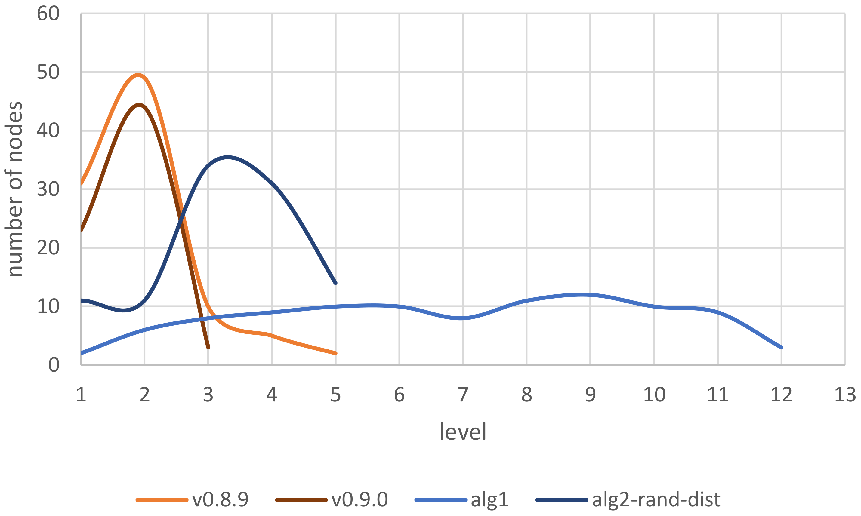
Figure 1. Node mapping and operations as a result of dissimilarity measures.
Computers 09 00035 g001
Figure 2. Node distribution in program versions. (a) Node distribution per level for 10 NewPipe program versions and average number of nodes for currently available versions; (b) Node distribution per level for available versions of five publicly available programs.
Computers 09 00035 g002
Figure 3. Tree height variation for Algorithm 1 variants.
Computers 09 00035 g003
Figure 4. Tree with 100 nodes generated by Algorithm 1.
Computers 09 00035 g004
Figure 5. Node distribution per level for generated trees (alg1, alg2-rand-dist) and NewPipe class hierarchy in versions 0.8.9 and 0.9.0.
Computers 09 00035 g005
Figure 6. Trees generated by node distribution and tree distortion: (a) by node distribution; (b) distorted from (a); (c) by node distribution equal to (a).
Computers 09 00035 g006
Figure 7. TED distance for increasing number of distortion parameters.
Computers 09 00035 g007
Table 1. Statistical values for trees representing class hierarchy in NewPipe versions 0.8.9 and 0.9.0.
v0.8.9v0.9.0
n9770
h53
N l 1/30/49/10/5/21/22/44/3
D a 30/1.63/0.2/0.5/0.4/022/2/0.07/ 0
d i s t [ % ] 31.25/51.04/10.42/5.21/2.0831.88/63.77/4.35
Table 2. Algorithm 1 steps for each algorithm variant.
StepRandom P-CRandom P-C with U n Random P Iterative CRandom P-C with U n / U s
[initialize] U n V ; u r getRandomNode(V); u r getRandomNode(V);
U n V { u r } ;
U s { u r } ;
[parent]getRandomNode(V);getRandomNode(V);getRandomNode(V);getRandomNode( U s );
[child]getRandomNode(V);getRandomNode( U n );getNextNode(V);getRandomNode( U n );
[condition] u p u c u p u c u r u c u p u c
u c getPreds( u p ) u c getPreds( u p ) u c getPreds( u p )
u p getPreds( u c )
[adjust] U n U n { u c } ; U n U n { u c } ;
U s U s { u c } ;
Table 3. Tree heights and equal hits (EH) for Algorithm 1 variants (avg(std.dev.)).
Algorithm VariantAvg. HeightAvg. EH
rand. P-C21.8021.029
[±4.979][±1.017]
rand. P-C with Un21.7461.045
[±4.951][±1.035]
rand. P iterative C24.5901.530
[±5.294][±1.487]
rand. P-C with Un/Us8.4710.000
[±1.312][±0.000]
Table 4. N l and D a with edit distance results for trees generated by Algorithms 1 and 3.
N l 1 N l 2 D a 1 D a 2 GEDTED
1/1/3/2/1/21/4/3/1/11/3/0.67/0.50/2/04/0.75/0.33/1/01214
1/2/2/3/1/11/4/2/2/12/1/1.50/0.33/1/04/0.50/1/0.50/01012
1/1/3/3/21/3/3/2/11/3/1/0,67/03/1/0.67/0.50/0910
1/2/3/2/1/11/3/4/1/12/1.50/0.67/0.50/1/03/1.33/0.25/1/0912
1/1/2/1/1/2/1/11/1/2/4/1/11/2/0.50/1/2/0.50/1/01/2/2/0.25/1/01110
1/2/2/2/2/11/3/3/2/12/1/1/1/0.50/03/1/0.67/0,50/01013
1/2/1/2/1/2/11/2/4/1/22/0.50/2/0.50/2/0.50/02/2/0.25/2/01214
1/1/4/3/11/5/3/11/4/0.75/0.33/05/0.60/0.33/01015
1/1/1/1/1/2/1/1/11/2/2/1/3/11/1/1/1/2/0.50/1/1/02/1/0.50/3/0.33/0913
1/1/2/3/2/11/2/2/3/21/2/1.50/0.67/0.50/02/1/1.50/0.67/01014
1/1.77/2.03/2.03/1.83/ 1.41/1.25/11/2.40/2.47/2.23/ 1.52/1.33/11.77/1.15/1/0.87/0.58/ 0.32/0.10/02.40/1.03/0.91/ 0.57/0.42/0.19/09.6 ±1.111.13 ±2.24
Table 5. Tree node distribution generated by Algorithm 2 ( T 1 ) and Algorithm 3 ( T 2 ).
T 1 Input Distribution T 1 Output T 2 Output by Distortion Parameters
(10, 10, 0.1)(50, 0, 0)(0, 50, 0)(0, 0, 0.5)
22.77%, 48.04%, 16.05%, 6.38%, 3.74%, 3.02% Computers 09 00035 i001 Computers 09 00035 i002 Computers 09 00035 i003 Computers 09 00035 i004 Computers 09 00035 i005
20%, …, 20% Computers 09 00035 i006 Computers 09 00035 i007 Computers 09 00035 i008 Computers 09 00035 i009 Computers 09 00035 i010
10%, …, 10% Computers 09 00035 i011 Computers 09 00035 i012 Computers 09 00035 i013 Computers 09 00035 i014 Computers 09 00035 i015
10%, 20%, 30%, 40% Computers 09 00035 i016 Computers 09 00035 i017 Computers 09 00035 i018 Computers 09 00035 i019 Computers 09 00035 i020
40%, 30%, 20%, 10% Computers 09 00035 i021 Computers 09 00035 i022 Computers 09 00035 i023 Computers 09 00035 i024 Computers 09 00035 i025
6.25%, 12.5%, 18.75%, 25%, 18.75%, 12.5%, 6.25%
3.9%, 6.3%, 7.8%, 8.75%, 9.15%, 9.35%, 9.5
Computers 09 00035 i026 Computers 09 00035 i027 Computers 09 00035 i028 Computers 09 00035 i029 Computers 09 00035 i030
9.35%, 9.15%, 8.75%, 7.8%, 6.3%, 3.9% Computers 09 00035 i031 Computers 09 00035 i032 Computers 09 00035 i033 Computers 09 00035 i034 Computers 09 00035 i035
Table 6. Generated data structure’s characteristics.
StructureNodes ConnectionSpecificsStructure TypeUsage
recursive tree [14]from rootinteger labelsunordered*
random binary tree [15,16]random inserttwo child nodesorderedbinary search
treap/randomized BST [17,18]add/delete opstwo child nodesorderedbinary search
random graphs [19,20]probability of connection**graph*
* various (e.g., networks, pattern recognition, biochemistry) ** general data structure.
Table 7. Characteristics of tree generation algorithms for comparison.
AlgorithmSimilarityDifferences
random (Algorithm 1)binary treesunordered, arbitrary number of child nodes
random (Algorithm 1) *recursive treesarbitrary labels
node distribution (Algorithm 2)graphsdistribution of nodes, unordered trees
distort (Algorithm 3)treap/randomized BSTunordered, arbitrary number of child nodes,
parent change operation
* Random P-C with U n / U s .

