Comparing Static and Dynamic Weighted Software Coupling Metrics ^†

Abstract

Coupling metrics that count the number of inter-module connections in a software system are an established way to measure internal software quality with respect to modularity. In addition to static metrics, which are obtained from the source or compiled code of a program, dynamic metrics use runtime data gathered, e.g., by monitoring a system in production. Dynamic metrics have been used to improve the accuracy of static metrics for object-oriented software. We study weighted dynamic coupling that takes into account how often a connection (e.g., a method call) is executed during a system’s run. We investigate the correlation between dynamic weighted metrics and their static counterparts. To compare the different metrics, we use data collected from four different experiments, each monitoring production use of a commercial software system over a period of four weeks. We observe an unexpected level of correlation between the static and the weighted dynamic case as well as revealing differences between class- and package-level analyses.

1. Introduction

Coupling [1,2]—the number of inter-module connections in software systems—has long been identified as a software architecture quality metric for modularity [3]. Taking coupling metrics into account during development of a software system can help to increase the system’s maintainability and understandability [4]. As a consequence, aiming for high cohesion and low coupling is accepted as a design guideline in software engineering [5].

In the literature, there exists a wide range of different approaches to defining and measuring coupling. Usually, the coupling degree of a module (class or package) indicates the number of connections it has to different system modules. A connection between modules $\mathbf{A}$ and $\mathbf{B}$ can be, among others, a method call from $\mathbf{A}$ to $\mathbf{B}$, a member variable from $\mathbf{A}$ of type $\mathbf{B}$, or an exception of type $\mathbf{B}$ thrown by $\mathbf{A}$. Many notions of coupling can be measured statically, based on either source code or compiled code.

Static analysis is attractive since it can be performed immediately on source code or on a compiled program. However, it has been observed [6,7,8] that for object-oriented software, static analysis does not suffice, as it often fails to account for effects of inheritance with polymorphism and dynamic binding. This is addressed by dynamic analysis, which uses monitoring logs generated while running the software. Dynamic analysis is often used to improve upon the accuracy of static analysis [9]. The results obtained by dynamic analysis depend on the workload used for the run of the system yielding the monitoring data. Hence, the availability of representative workload for the system under test is crucial for dynamic analysis. As a consequence, dynamic analysis is more expensive than static analysis.

Dynamic analysis uses the recorded data to find, e.g., all classes $\mathbf{B}$ whose methods are called by the class $\mathbf{A}$. In this case, the individual relationship between two classes $\mathbf{A}$ and $\mathbf{B}$ is qualitative: The analysis only determines whether there is a connection between $\mathbf{A}$ and $\mathbf{B}$, and does not take its strength (e.g., number of calls during a system’s run) into account. In contrast to such a qualitative metric, a quantitative coupling measurement quantifies the strength (measured, e.g., as the number of corresponding method calls during runtime of the system) of the connection between $\mathbf{A}$ and $\mathbf{B}$ by assigning it a concrete number. In this paper, we study such quantitative metrics.

The coupling metrics we consider in this paper are defined using a dependency graph. The nodes of such a graph are program modules. Edges between modules express call relationships. They can be labelled with weights, which are integers denoting the strength of the connection (i.e., the number of occurrences of the call represented by the edge). Depending on whether coupling metrics take these weights into account or not, we call the metrics weighted or unweighted. The main two metrics we consider in this paper are the following:

• Unweighted static coupling, where an edge from $\mathbf{A}$ to $\mathbf{B}$ is present in the dependency graph if some method from $\mathbf{B}$ is called from $\mathbf{A}$ in the (source or compiled) program code—independently of how many different methods in $\mathbf{A}$ call how many different methods in $\mathbf{B}$, there is only a single edge (or none) from $\mathbf{A}$ to $\mathbf{B}$ in this unweighted metric.
• Weighted dynamic coupling, where an edge from $\mathbf{A}$ to $\mathbf{B}$ is present in the graph if such a call actually occurs during the monitored run of the system, and is attributed with the number of such calls observed.

We also consider, as an intermediate metric between these two, an unweighted dynamic coupling metric.

Dynamic weighted coupling measures cannot replace their static counterparts in their role to, e.g., indicate maintainability of software projects. However, we expect dynamic weighted coupling measures to be highly relevant for software restructuring. In contrast to static coupling measures, weighted dynamic measures can reflect the runtime communication “hot spots” within a system, and therefore may be helpful in establishing performance predictions of restructuring steps. For example, method calls that happen infrequently can possibly be replaced by a sequence of nested calls or with a network query without relevant performance impacts. Since static coupling measures are often used as basis for restructuring decisions [5,10], dynamic weighted coupling measures can potentially complement their static counterparts in the restructuring process. This possible application leads to the following question: Do dynamic coupling measures yield additional information beyond what we can obtain from static analysis? More generally, what is the relationship between dynamic and static coupling measures?

The main research question we investigate in this paper is: Are static coupling degrees and dynamic weighted coupling degrees of a software system statistically independent? If we observe correlation, can we quantify the correlation?

Initially, we expected the answer to be say, since we believed static and dynamic coupling degrees to be almost unrelated: A module $\mathbf{A}$ has high static coupling degree if there are many method calls from methods in $\mathbf{A}$ to methods outside of $\mathbf{A}$ or vice versa in the program code. On the other hand, $\mathbf{A}$ has high dynamic weighted coupling degree if during the observed run of the system, there are many runtime method calls between $\mathbf{A}$ and other parts of the system. Since a single occurrence of a method call in the code can be executed millions of times—or not at all—during a run of the program, static and weighted dynamic coupling degrees do not need to correlate, if we observe a large number of method calls. Thus, our initial hypothesis was to not observe a high correlation between static and weighted dynamic metrics.

To answer these questions, we compare the two coupling measures. We use dynamically collected data to compute weighted metrics that take into account the number of function calls during the system’s run. We obtained the data from a series of four experiments. Each experiment consists of monitoring real production usage of a commercial software system (Atlassian Jira [11]) over a period of four weeks each. Our monitoring data, of which we have made an anonymized version publically available [12,13,14,15], contains more than three billion method calls.

To address our main research question, we compare the results from our dynamic analysis to computations of static coupling degrees. Directly comparing static and weighted dynamic coupling degrees is of little value, as these are fundamentally different measurements. For instance, the absolute value of dynamic weighted degrees depends on the duration of the monitored program run, which clearly is not the case for the static measures (Table 10 shows the average coupling degrees we obtained during our four experiments, these numbers illustrate the effect of longer runs of a system on dynamic coupling degrees). We therefore instead compare coupling orders, i.e., the ranking obtained by ordering all program modules by their coupling degree using the Kendall–Tau (See [16] for a discussion of the relationship between this metric and Spearman’s correlation) metric [17]. This also allows to quantify the difference between such orders.

Our answer to the above stated research questions is that static and (weighted) dynamic coupling degrees are not statistically independent. This result is supported by 72 individual comparisons. A possible interpretation of this result is that dynamic weighted coupling degrees give additional, but related information compared to the static case. In addition to this result, we observe insightful differences between class- and package-level analyses.

1.1. Contributions

The results and contributions of this paper are:

• Using a unified framework, we introduce precise definitions of static and dynamic coupling measures.
• We investigate our new coupling definitions with regard to the axiomatic framework presented in [18].
• To investigate our main research question, we performed four experiments involving real users of a commercial software product (the Atlassian Jira project and issue tracking tool [11]) over a period of four weeks each. The software was instrumented with the monitoring framework Kieker [19], a dynamic monitoring framework based on AspectJ [20]. From the collected data, we computed our dynamic coupling measures. Using the Kendall–Tau metric [17,21], we compared the obtained results to coupling measures we obtained by static analysis.
• We puslished the data collected in our experiments on Zenodo [12,13,14,15], and provide a small tool as a template for a custom analysis of the datasets [22].
• Our results show that all coupling metrics we investigate are correlated, but there are also significant differences. In particular, when considering package-level coupling, the correlation is significantly stronger than for class-level coupling. We assume that effects like polymorphism and dynamic binding often do not cross package boundaries.

This paper is an extended version of our conference paper [23]. Compared to the conference publication, the current paper contains extended discussion and interpretation, additional references, and the following additional results:

• we analyzed our newly proposed metrics with regard to the framework proposed by Briand et al. [18].
• as companion artifacts to this paper, we published anonymized versions of the data obtained in our experiments on the open-access repository Zenodo. In Section 7, we provide a detailed description of the data as well as a reference to a template program that allows to access our data as a further companion artifact.

1.2. Paper Organization

The remainder of the paper is organized as follows: In Section 2, we discuss related work. Section 3 provides our definition of weighted dynamic coupling. In Section 4, we explain our approach to static and dynamic analysis. Section 5 then describes the setting of our experiment. The results are presented and discussed in Section 6. Section 7 describes the data collected during our experiments, which is accessible on Zenodo. In Section 8, we discuss threats to validity and conclude in Section 9 with a discussion of possible future work.

2. Related Work

There is extensive literature on using coupling metrics to analyze software quality, see, e.g., Fregnan et al. [24] for an overview. Briand et al. [25] propose a repeatable analysis procedure to investigate coupling relationships. Nagappan et al. [26] show correlation between metrics and external code quality (failure prediction). They argue that no single metric provides enough information (see also Voas and Kuhn [27]), but that for each project a specific set of metrics can be found that can then be used in this project to predict failures for new or changed classes. Misra et al. [28] propose a framework for the evaluation and validation of software complexity measures. Briand and Wüst [29] study the relationship between software quality models (of which coupling metrics are an example) to external qualities like reliability and maintainability. They conclude that, among others, import and export coupling appear to be useful predictors of fault-proneness. Static weighted coupling measures have been considered by Offutt et al. [30]. Allier et al. [31] compare static and unweighted dynamic metrics.

Many of the above-mentioned papers study the relationship between coupling and similar software metrics and quality notions for software. Our approach is different: We do not study correlation between software metrics and software quality, but correlation between different software metrics, namely static and dynamic coupling metrics.

Dynamic (unweighted) metrics have been investigated in numerous papers (see, e.g., Arisholm et al. [8] as a starting point, also the surveys by Chhabra and Gupta [32] and Geetika and Singh [33]). Dynamic analysis is often used to complement static analysis. None of these approaches considers dynamic weighted metrics, as we do.

As an notable exception, Yacoub et al. [34] use weighted metrics. However, to obtain the data, they do not use runtime instrumentation—as we do—but “early-stage executable models.” They also assume a fixed number of objects during the software’s runtime.

Arisholm et al. [8] study dynamic metrics for object-oriented software. Our dynamic coupling metrics are based on their dynamic messages metric. The difference is as follows: Their metric counts only distinct messages, i.e., each method call is only counted once, even if it appears many times in a concrete run of the system. The main feature of our weighted metrics is that the number of occurrences of each call during the run of a system is counted. The dynamic messages metric from [8] corresponds to our unweighted dynamic coupling metrics (see below).

3. Dynamic, Weighted Coupling

3.1. Goals and Techniques for Dynamic Metrics

As discussed in the introduction, the main question we study in this paper is whether weighted dynamic and static coupling metrics are statistically independent. In order to be able to perform a conclusive comparison, we study metrics that assign a coupling degree to each module (i.e., class or package).

A straight way to measure the coupling degree of a module $\mathbf{A}$ is to count the number (or ratio) of messages involving $\mathbf{A}$. Our coupling measures are all based on this idea. In addition, we can distinguish between messages sent or received by $\mathbf{A}$ (these constitute import or export coupling) or count both (combined coupling). In all coupling measures, we always skip reflexive messages that a module sends to itself, since we are interested in coupling as a way to express relationships and dependencies between different program modules.

Note that while object-level coupling is an interesting topic by itself, objects only exist at runtime and hence object-level coupling cannot be measured with static analysis. Therefore, object-level analysis cannot be used to compare the relationship between dynamic and static coupling, and hence in the present paper we focus on coupling aggregated to the class respective package level.

3.2. Dependency Graph Definition

We performed our analyses with two different levels of granularity: on the (Java) class and package levels. Since the approach is the same for both cases, in the following we use the term module for either class or package, depending on the granularity of the analysis. The raw output of either types of analyses (dynamic and static) is a labeled, directed graph G, where the nodes represent program modules, and the labels are integers which we refer to as weights of the edges. If an edge from $\mathbf{A}$ to $\mathbf{B}$ has label (weight) $n_{A,B}$, this denotes that the number of directed interactions between $\mathbf{A}$ and $\mathbf{B}$ occurring in the analysis is $n_{A,B}$.

In the case of a static analysis, this means that there are $n_{A,B}$ places in the code of $\mathbf{A}$ where some method from $\mathbf{B}$ is called. For dynamic analysis, this means that during the monitored run of the system, there were $n_{A,B}$ run-time invocations of methods from $\mathbf{B}$ by methods from $\mathbf{A}$.

When we disregard the numbers $n_{A,B}$, the graph G is a plain dependency graph: Such a graph is a directed graph, where each node is a module, and edges reflect function calls between the modules. Dependency graphs are standard in the analysis of coupling metrics. Since we also take the weights $n_{A,B}$ into account, our graph G is a weighted dependency graph, hence we call the coupling metrics we define below weighted metrics. Analogously, we will refer to metrics defined on the unweighted dependency graph—i.e., metrics that do not take the weights $n_{A.B}$ into account—as unweighted metrics. See Section 3.3 below for examples of the dependency graphs used in our metrics definitions. In the sequel, we study weighted metrics only for the dynamic case (although, as seen above, they can be defined for the static case as well). We therefore have the following three conceptually different approaches to measure coupling dependency between program modules:

• The first approach is static analysis, which identifies method calls by analyzing the compiled code (where the data is obtained by a static analysis tool—in our case, we used BCEL [35] to analyze Java .class and .jar files). As usual in the case of static analysis, here we do not take weights into account. We therefore compute our static coupling measures from an unweighted dependency graph.
• Our second approach is unweighted dynamic analysis. This analysis identifies method calls between modules as they appear in an actual run of the system (the data is obtained by monitoring), but does not take the weights $n_{A,B}$ into account. It therefore does not distinguish between cases where a module $\mathbf{A}$ calls another module $\mathbf{B}$ a million times or just once. This metric is essentially the dynamic messages metric from [8].
• Our third approach is weighted dynamic analysis, which differs from its unweighted counterpart only by taking the weights $n_{A,B}$ into account.

The distinctions between static/dynamic analyses and unweighted/weighted analyses are orthogonal choices. In particular, we omit in the present paper a weighted, static analysis, since our main motivation is the comparison of dynamic, weighted metrics to unweighted, static metrics. We consider the dynamic, unweighted metric to be the more interesting intermediate step due to the following reasons:

• Dynamic, unweighted metrics are interesting on their own, and were, e.g., discussed in [8] as dynamic messages.
• Defining and measuring weighted, static coupling metrics is arguably less natural than the other three metrics: To measure static, weighted coupling, we need to count, e.g., occurrences of method calls from some class $\mathbf{A}$ to a method m of class $\mathbf{B}$. However, the number of method calls is not invariant under equivalence-maintaining transformations, e.g., rewriting case distinctions or looping constructs. In particular, when analyzing byte code as opposed to source code, the result can depend on the compiler optimization (see also Section 4.1).

We therefore omit weighted static coupling from our analysis in this paper.

Our three basic approaches are applied in class and package granularities, and for three different types of coupling (import-, export- and combined coupling), therefore each experiment results in 18 different analyses. We treat the three basic approaches uniformly by treating the unweighted dependency graph as a special case of the weighted graph, where all weights are 1. This allows us to define all our coupling metrics using the weighted dependency graph as input.

3.3. Dependency Graphs Examples

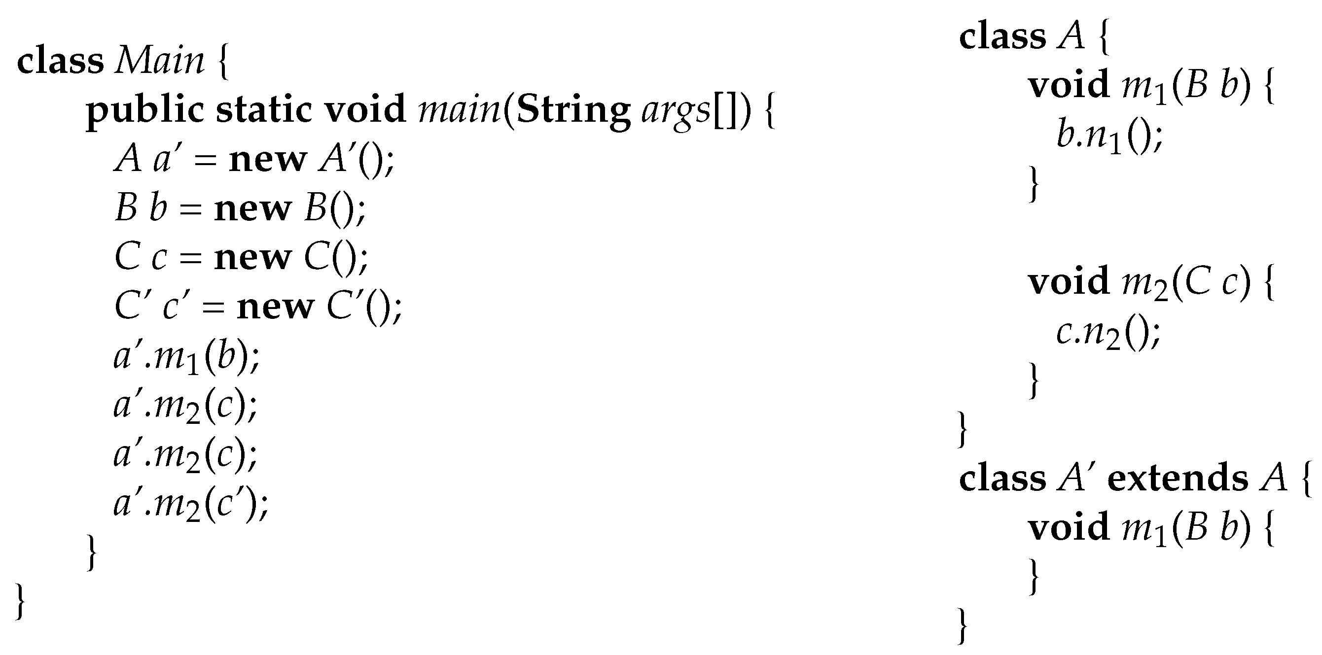
We now give an example to illustrate the different variations of dependency graphs we use in this paper. For this, consider the example Java source code presented in Figure 1. The source code contains the three classes Main, A, and A′, where A′ is a subclass of A. There are three additional classes for which we do not present the source code: These are B, C, and C′, where C′ is a subclass of C. In B, a method n${}_1$ is specified, in C, a method n${}_2$ is specified; n${}_2$ is inherited by C′. These methods only call methods internal to their containing class, and therefore do not contribute to the dependency graph—therefore we omit their source code. All classes we present here are in the same Java package, as we consider coupling on the class level. We focus on import coupling in the following discussion, the graphs for export coupling are obtained from the ones for import coupling by reversing the directions of all arrows, the ones for combined coupling are obtained from the other two by adding the weights on their edges.

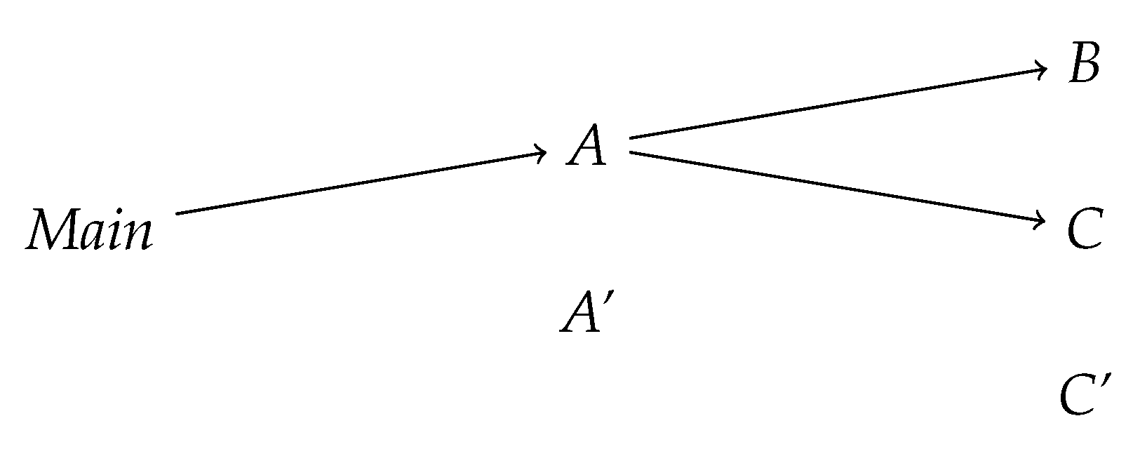
We will now demonstrate the three dependency graphs induced by the above program. In the following, we will only draw edges that have a non-zero label. We start with the static dependency graph, presented in Figure 2. Recall that we measure only unweighted static coupling, therefore the edges in this graph do not have labels (implicitly, the weights are treated as 1). Also, recall that we do not consider self-calls, i.e., reflexive edges in the graph. In the static graph, there are calls from Main to methods from A, but not to A′, since the variable a is of type A (even though it is instantiated with an object of type A′). From A, there are edges to B and to C, since the code of A calls methods B.m${}_1$ and C.m${}_2$.

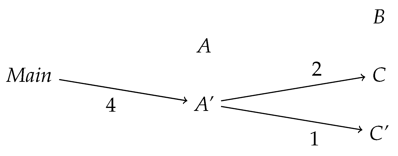
Next, we consider the weighted, dynamic dependency graph, see Figure 3. This graph differs from the static one, since calls present in the static analysis can be modified or left out in the running program: Calls made to C in the method m${}_2$ can be replaced with calls to C′, if c is instantiated with an object of type C′ or skipped altogether (since the implementation of m${}_1$ in A′ does not perform any method calls). This is detected by dynamic analysis, since here we follow the program execution and not merely its structure.

In the example code starting at the main method, we have 4 calls from Main to A′, as 4 methods of the object $a^{\prime }$ (of type A′) are called, and no call from Main to A, even though of course the method m${}_2$ in A′ is in fact implemented in the class A. There are no outgoing edges from the class A, since no object of type A is created during the program run. The method a′.m${}_1$(b) does not result in a method call from A or A′ to B or B′, since the method m${}_1$ of A′ (which is executed in this case) does not perform any operations on the object b. The method calls a′.m${}_2$(c) (performed twice) and a’.m${}_2$(c′) result in two calls from A′ to C and a single call from A′ to C′, since the method m${}_2$ calls a method from the object c.

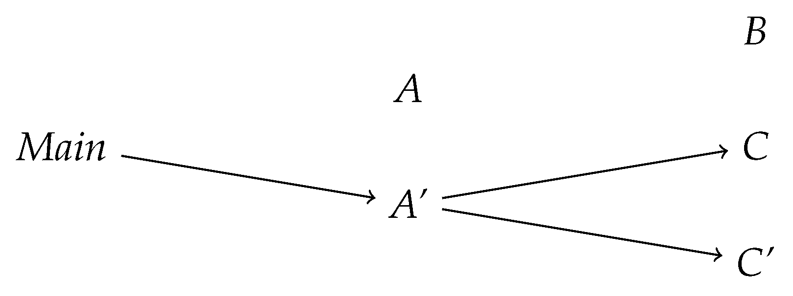
Finally, the unweighted dynamic dependency graph (Figure 4) is obtained from its weighted counterpart by simply removing the labels (the weights are implicitly understood to be 1 in an unweighted graph).

In this toy example, the edges between the static and the dynamic graphs are disjoint, i.e., there is no edge that appears in both graphs. Clearly, in most real examples the differences between static and dynamic dependency graphs will be smaller.

3.4. Definition of Coupling Metrics

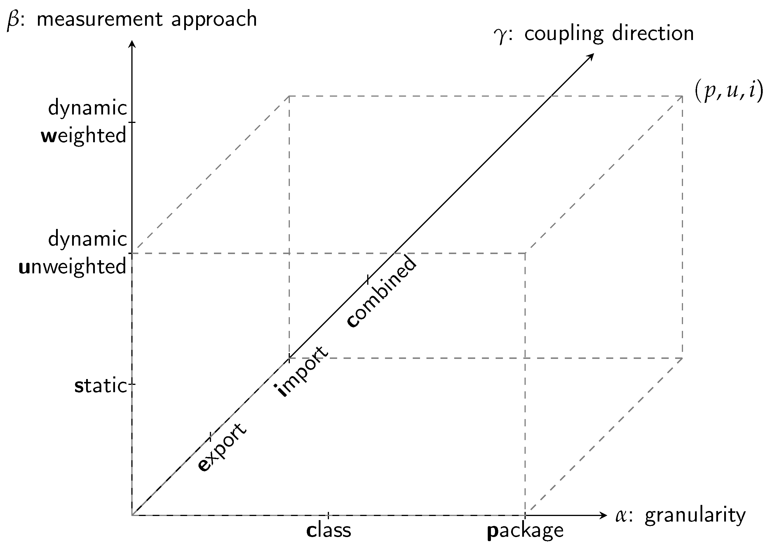
We now define the coupling measures we study in this paper. Our measures assign a coupling degree to a program module (i.e., a class or a package). As discussed in Section 3.2, we consider 18 different ways to measure coupling, resulting from the following three orthogonal choices:

• The first choice is between class-level and package-level granularity. Depending on this choice, a module is either a (Java) class or a (Java) package.
• The second choice is between one of our three basic measurement approaches: static, dynamic unweighted, or dynamic weighted analysis.
• The third choice is to measure import-, export- or combined-coupling.

To distinguish these 18 types of measurement, we use triples $(\alpha ,\beta ,\gamma )$, where $\alpha$ is c or p and indicates the granularity, $\beta$ is s, u, or w and indicates the basic measurement approach, and $\gamma$ is i, e, or c, indicating the direction of couplings taken into account. Figure 5 illustrates these three orthogonal choices: The example triple $(p,u,i)$ denotes an analysis with granularity package-level, using dynamic unweighted analysis, and considers coupling in the import direction.

As discussed in Section 3.2, all of our coupling measures can be computed from the two dependency graphs resulting from our two analyses (static and dynamic). In the static and dynamic unweighted analysis cases, we replace each weight $n_{A,B}$ with the number 1. For a module $\mathbf{A}$, and a choice of measure $(\alpha ,\beta ,\gamma )$, the $(\alpha ,\beta ,\gamma )$-coupling degree of $\mathbf{A}$, denoted with ${\mathsf{coupdeg}}_{\alpha ,\beta ,\gamma }\left(\mathbf{A}\right)$, is computed as follows:

• We compute $G_{\alpha ,\beta }$. This is the weighted dependency graph between classes (if $\alpha =c$) or packages (if $\alpha =p$) obtained by static analysis (if $\beta =s$) or dynamic analysis (if $\beta =u$ or $\beta =w$), where each weight $n_{A,B}$ is replaced with 1 if the analysis is static or dynamic unweighted (i.e., if $\beta \in \left\{s,u\right\}$).
• Then, ${\mathsf{coupdeg}}_{\alpha ,\beta ,\gamma }\left(\mathbf{A}\right)$ is obtained as the out-degree of $\mathbf{A}$, in-degree of $\mathbf{A}$, or sum of these two, depending on whether $\gamma =i$, $\gamma =e$, or $\gamma =c$. Here, the in (out) degree of a node is the sum of the weights of its incoming (outgoing) edges in the graph. Since we replace all weights with 1 for the unweighted analyses, we obtain the usual definition of degrees in unweighted graphs in these cases.

3.5. Analysis of Dynamic Coupling Metrics with Respect to Framework by Briand et al.

Chhabra and Gupta [32] mention that most existing dynamic metrics do not fall into the axiomatic framework of Briand et al. [18] (see also Arisholm et al. [8]). Below, we study our proposed metrics definitions with respect to the conditions required by this framework. We show that our metrics satisfy all of these conditions, except for monotonicity. However, a version of monotonicity adapted to the dynamic setting is satisfied by our measures, as explained below. The fact that our metrics essentially satisfy the conditions indicate that our definitions are in fact natural notions of coupling. In the following, let ${\mathsf{coupdeg}}_{\alpha ,\beta ,\gamma }(.)$ be one of the 18 coupling measures defined above (i.e., $\alpha \in \left\{c,p\right\}$, $\beta \in \left\{s,u,w\right\}$, and $\gamma \in \left\{i,e,c\right\}$).

3.5.1. Nonnegativity and Null Values

Nonnegativity requires that ${\mathsf{coupdeg}}_{\alpha ,\beta ,\gamma }\left(A\right)$ is never negative for any class or package $\mathbf{A}$. The null value requirement states that the value is zero if and only if the set of outgoing, resp., incoming or both messages of $\mathbf{A}$ is empty. Both properties are obviously satisfied by the definition of our measures.

3.5.2. Monotonicity

This requires that if a class $\mathbf{A}$ is modified such that one or more instances of $\mathbf{A}$ sends or receives more messages, then ${\mathsf{coupdeg}}_{\alpha ,\beta ,\gamma }\left(A\right)$ cannot decrease.

This requirement is usually satisfied in coupling definitions for static analysis, and this is obviously the case for ${\mathsf{coupdeg}}_{\alpha ,\beta ,\gamma }(.)$ if $\alpha =s$, i.e., our metric for static analysis.

In the dynamic case, the situation is more complex: The condition requires to compare two evaluations of the coupling degree. For a dynamic analysis, two different runs of the system have to be considered: one with the original implementation of $\mathbf{A}$, and one with the modification. However, changing the implementation of $\mathbf{A}$ can change the behaviour of the system: A new function call (i.e., a sent message) added to $\mathbf{A}$ can let the system follow a completely different behaviour, in which $\mathbf{A}$’s code is not called anymore after the first occurrence of the new message. This can reduce the value of ${\mathsf{coupdeg}}_{\alpha ,\beta ,\gamma }\left(A\right)$. This issue is unrelated to the used workload. In particular, it remains when we use the same user behaviour for both implementations of the system.

However, a natural interpretation of the monotonicity requirement in the dynamic setting would be the following: Instead of comparing two different implementations of $\mathbf{A}$ and the resulting (possibly completely different) runs of the system, we can compare two weighted dependency graphs $G_1$ and $G_2$, where $G_2$ is obtained from $G_1$ by increasing the weight (for simplicity, treat absent edges as edges with weight 0) of the edge $(\mathbf{A},X)$ or $(X,\mathbf{A})$ (depending on the direction of coupling we consider), and compute ${\mathsf{coupdeg}}_{\alpha ,\beta ,\gamma }\left(A\right)$ based on $G_1$ and $G_2$. In this case, the measure computed on $G_2$ is obviously not smaller than the one computed on $G_1$, hence this dynamic interpretation of monotonicity is satisfied.

3.5.3. Impact of Merging Classes

This property requires that if classes $\mathbf{A}$ and $\mathbf{B}$ are merged into the new class $\mathbf{AB}$, then the coupling measure satisfies ${\mathsf{coupdeg}}_{\alpha ,\beta ,\gamma }\left(A\right)+{\mathsf{coupdeg}}_{\alpha ,\beta ,\gamma }\left(B\right)\ge {\mathsf{coupdeg}}_{\alpha ,\beta ,\gamma }\left(AB\right)$.

This property is obviously satisfied: The dependency graph $G_{\alpha ,\beta }$ of the new system $S^{\prime }$ is essentially obtained from the one for the old system S by re-routing messages involving $\mathbf{A}$ or $\mathbf{B}$ to $\mathbf{AB}$, and removing all messages exchanged between $\mathbf{A}$ and $\mathbf{B}$ (in the new system $S^{\prime }$, these messages are now internal messages of $\mathbf{AB}$ and therefore are not counted).

3.5.4. Merging Uncoupled Classes

This requirement states that, in the above-studied merging scenario, if there are no messages exchanged between $\mathbf{A}$ and $\mathbf{B}$, then the above inequality is strengthened to the equality

$${\mathsf{coupdeg}}_{\alpha ,\beta ,\gamma }\left(A\right)+{\mathsf{coupdeg}}_{\alpha ,\beta ,\gamma }\left(B\right)={\mathsf{coupdeg}}_{\alpha ,\beta ,\gamma }\left(AB\right).$$

This obviously holds true following the above argumentation, as there exists no message between $\mathbf{A}$ and $\mathbf{B}$ that is rerouted to become an internal message of $\mathbf{AB}$. Note that clearly, there can be internal messages of $\mathbf{AB}$ in the new system $S^{\prime }$, since there may be internal messages of $\mathbf{A}$ or $\mathbf{B}$ in the original system S.

3.5.5. Symmetry between Import/Export Coupling

This property requires the sum over all export couplings to equal the sum over all import couplings, this is obvious for our definitions.

4. Static and Dynamic Analysis

The main goal of this paper is to compare static and dynamic analyses via experiments measuring a software system in production use (see Section 5 for the experiment’s description). We start by explaining the techniques used to obtain both the static and the dynamic measurements.

4.1. Static Analysis

Since we monitor a commercial product where the source code is not available (see Section 5.1), we perform static analysis on the compiled code. For this, we apply the Apache BCEL (Byte Code Engineering Library) [35] that allows to inspect the Java class files from our installation of the software. BCEL allows to parse Java class files on the statement level. We use it to identify every method call between different classes to construct our (static) dependency graph.

Note that one consequence of using compiled code is that some optimizations have already performed by the compiler, such as removal of dead code. Therefore, our static and dynamic analysis are performed on the exact same code, without differences introduced in the compilation process.

4.2. Dynamic Analysis

For our dynamic analysis, we use the Kieker Monitoring Framework [19,36,37], which is designed to perform dynamic analysis of programs running on the Java Virtual Machine (JVM). Its measurement methods are highly configurable. Our Jira installation was instrumented with probes that can register every method call.

Inevitably, dynamic monitoring adds overhead to the system under test, since the additional monitoring code is performed within the process of the monitored software, even though the Kieker framework we use has a low impact on performance [38], In order to maintain responsiveness of the system in our real-life setting, we limited the monitoring to the core functionality of the software. For example, the system’s own logging subsystem and some classes were excluded from our monitoring due to technical reasons. We took these restrictions into account for the comparative evaluation of our static and dynamic analysis.

4.3. Fine-Tuning

Our analyses are highly configurable (the static analysis is a custom Java program using the BCEL library, Kieker’s dynamic monitoring can be configured using different pointcuts and probes to monitor various combinations of events). This allowed us to fine-tune both analyses to ensure that they indeed result in comparable measurements. In both the static and the dynamic analysis cases, we counted Java method calls between different classes/packages, excluding constructor calls.

5. Experiment Design

5.1. System under Test and Test Conditions

We analyzed the software Atlassian Jira, versions 7.3.0, 7.4.3, and 7.7.1 [11]. Jira is an issue management tool allowing (among other features) the management of Scrum and Kanban software development processes [39]. The system was instrumented using Kieker (see Section 4.2). For each method call, we recorded the time stamp, the class name of caller and of the callee, as well as object identifiers allowing for object-level analysis (object-level analysis is not covered in this paper but left for future research).

5.2. Workload

Static coupling analyses can be performed on either the source code or the compiled program (see Section 4.1) in a usually straight forward and inexpensive way. In contrast, dynamic analysis requires a running system and appropriate workload for it [40]. This is particularly important for a weighted analysis, because multiple runs of the same code have an effect only for weighted measurements. In an unweighted analysis, repeating parts of a run do not change the dependency graph, as no new edges are introduced. In a weighted analysis, however, the weights on the relevant edges are increased by running even the exact same sequence of method calls again. Therefore, having realistic workload (either from real users or from a workload generator) is crucial for weighted, dynamic metrics.

To perform our analysis with realistic workload, we conducted four experiments with real users using a software system (Atlassian Jira [11]) in production. We deployed Jira on our own servers in order to perform monitoring. The Jira installation was used by students participating in a mandatory programming course of our computer science curriculum. In the course, the students develop a software using the Kanban process management method [39]. The time span of the project is four weeks, with full time participation by the students. The students mainly used Jira’s Kanban board and issue tracking features. Hence, the analysis only covers a subset of Jira’s capabilities, and thus classes of its implementation.

We report on four experiment runs, from February and September of 2017 and 2018. Each time, the software ran for a four-week period. The collected monitoring data from each run includes the startup sequence, basic configuration such as database access, initial tasks as user registration and setup of the Kanban boards, and day-to-day usage. No person-related data is used for our analysis. In

Table 1. Numbers of users and monitored calls.

#	Date	Users	Method Calls
1	February 2017	19	196,442,044
2	September 2017	48	854,657,027
3	February 2018	16	475,357,185
4	September 2018	58	2,409,688,701

, we list the number of method calls recorded as well as the number of users of our Jira installation in each of the four experiment runs.

Obviously, there are differences between the four runs of the software that we analyze. For example, different students took parts in the course each time, the focus of the project required using different features of the Jira software in each iteration, and we also instructed the participants to use more features of the tool in the later iterations (this is one reason why the number of method calls per student is higher in the later runs of the experiment). Also, different versions of Jira were used in order to let students use features of the newer versions. Therefore, our four experiments—even though they are conducted using the same software system—give us slightly more variation in the data than running the exact same software with the exact same group of users. However, our main analysis results (see Section 6.1) do not vary significantly between the different runs of the experiment, indicating that our findings are invariant under small changes of the experiment setup.

Anonymized versions of the four datasets used in this study have been published on Zenodo. The later Section 7 describes the datasets and ways to access them in detail.

6. Experiment Results

The collected data from the experiment’s dynamic analysis, in addition with the static analysis, allows computing all 18 variations of ${\mathsf{coupdeg}}_{\alpha ,\beta ,\gamma }(.)$ as defined in Section 3.4. Therefore, the analyses yield 18 different measurements for each run of the experiment.

6.1. Comparing Static and Dynamic Coupling

As discussed previously, the central goal of this paper is to study the relationship between static and dynamic couplings, in particular between the static and dynamic weighted measures. We now present the results on these comparisons.

Recall that we study three fundamentally different ways to measure coupling degree: We perform static and dynamic measurements, where in the dynamic case, we look at both unweighted and weighted measures. While the main topic of this paper is the study of weighted metrics, we consider the unweighted dynamic case relevant for mainly two reasons:

• Dynamic unweighted coupling measures have been studied before [8,33]. Their main motivation to consider dynamic metrics were difficulties in precisely capturing object-oriented features with static analysis. Therefore, dynamic unweighted coupling analysis is an established measurement, and hence comparing our weighted dynamic metrics to the unweighted dynamic case is an original research question in itself.
• Dynamic unweighted coupling can be seen as “middle ground” between static and dynamic weighted coupling, as our static measurements are unweighted as well.

Intuitively, static and dynamic unweighted coupling measures are quite similar. A first intuition could be to assume that—measuring arbitrarily long runs of the system—the dynamic unweighted analysis will eventually converge to the static analysis: For a “complete” run of the system performing every method call present in the source or compiled code at least once, one could expect the static and unweighted dynamic analysis to coincide. However, this intuition is misleading due to (among others) the following reasons:

• In many software projects, there is “dead code,” i.e., (possible) function calls which are found by the static analysis, but are never executed in any real run of the system. Such function calls hence do not appear in the monitoring logs created for the dynamic analysis, independently of the user behaviour.
• It is well-known [6,7] that static analysis can be imprecise in an object-oriented context as it cannot take into account information available only at runtime (e.g., the actual type of an object that receives a message call, which may be a subtype of the type available to the static analysis).

Hence, even in a (hypothetical) “complete” run of a system, there would still be differences between static and dynamic unweighted analyses. Additionally, in a real system run, not all possible calls of a system will be made. Therefore, a significant difference between the results from static analysis and dynamic unweighted analysis is to be expected.

However, it is reasonable to assume that the above-described differences lead to smaller distances than the conceptual difference between unweighted and weighted analysis.

6.1.1. Compared Measures

To answer our main research question—whether static and dynamic weighted coupling are statistically independent—we compare the coupling degrees computed by these different approaches. Comparing the actual “raw” values of ${\mathsf{coupdeg}}_{\alpha ,\beta ,\gamma }\left(\mathbf{A}\right)$ for different combinations of $\alpha$, $\beta$, $\gamma$ and some class or package $\mathbf{A}$ does not make much sense: The weighted values depend on the length of the measurement run of the system, whereas the static analysis does not.

However, for a developer, the absolute coupling values are usually less interesting than the identification of the modules with the highest coupling degree. Therefore, a useful approach is to study the relationship between the orders among the modules in the different analyses. Each analysis yields an ordering of the classes or packages from the ones with the highest coupling degree to the ones with the lowest one; we call these orders coupling orders. These orders can be compared between different analyses of varying measurement durations.

Given our coupling measure definitions, we have the following choices for a left-hand-side (LHS) and a right-hand-side (RHS) analysis:

• The first choice is whether to consider class or package analyses (both the LHS and the RHS should consider the same type of module).
• The second choice is which two of our three basic measurement approaches (see Section 3.2) we intend to compare: static analysis, (dynamic) unweighted analysis, and (dynamic) weighted analysis. There are three possible choices: s vs u, s vs w, and u vs w.
• For each combination, we consider import, export, and combined coupling.

Hence, there are 18 comparisons we can perform in each of our four data sets, leading to 72 different comparisons (we do not compare coupling orders resulting from different runs of the experiments to each other). In the following, we explain our approach to comparing these coupling orders and report our findings.

6.1.2. Kendall–Tau Distance

To study the difference between our different basic measurement approaches, we compare the coupling orders of the analyses. An established way to measure the distance between orders (on the same base set of elements) is the Kendall–Tau distance [21], which is defined as follows: For a finite base set S with size n, the metric compares two linear orders ${<}_1$ and ${<}_2$. The Kendall–Tau distance $\tau ({<}_1,{<}_2)$ is the number of swaps needed to obtain the order ${<}_1$ from ${<}_2$, normalized by dividing by number of possible swaps $\frac{n(n-1)}{2}$. Hence, $\tau ({<}_1,{<}_2)$ is always between 0 (if ${<}_1$ and ${<}_2$ are identical) and 1 (if ${<}_1$ is the reverse of ${<}_2$). Values smaller than $0.5$ indicate that the orders are closer together than expected from two random orders, while values larger than $0.5$ indicate the opposite. Values further away from $0.5$ imply higher correlation between two orders.

There are also weighted refinements of the Kendall–Tau distance ([41], see also [42]), that are sometimes used in the context of software metrics. These weighted versions allow to, e.g., give more weight to elements appearing at the very “top” or “bottom” of the orders, i.e., in our case, to the most- or least-coupled classes or packages occurring in the analysis. While this is certainly an interesting approach, in the current paper we are more interested in the basic question to analyze the relationship between the static and dynamic analysis cases. So, for this paper, we use the standard Kendall–Tau distance and leave an analysis focused on the most (or least) coupled classes or packages for future work.

6.1.3. Distance Values and Statistical Significance

To present our results, we use the following notation to specify the LHS and RHS analyses: We use a triple $\alpha :{\beta }_1\leftrightarrow {\beta }_2$, where

• $\alpha$ is c or p expressing class or package coupling,
• ${\beta }_1$ is s or u expressing whether the LHS analysis is static or (dynamic) unweighted,
• ${\beta }_2$ is u or w expressing whether the RHS analysis is (dynamic) unweighted or (dynamic) weighted.

For each of these combinations, we consider export, import, and combined coupling analyses. This results in 18 comparisons for each data set, the results of which are presented in

Table 2. Coupling Analyses (Data Set 1).

	$\mathit{c}:\mathit{s}\leftrightarrow \mathit{u}$	$\mathit{c}:\mathit{s}\leftrightarrow \mathit{w}$	$\mathit{c}:\mathit{u}\leftrightarrow \mathit{w}$	$\mathit{p}:\mathit{s}\leftrightarrow \mathit{u}$	$\mathit{p}:\mathit{s}\leftrightarrow \mathit{w}$	$\mathit{p}:\mathit{u}\leftrightarrow \mathit{w}$
import	0.30	0.36	0.13	0.33	0.36	0.08
export	0.41	0.41	0.24	0.30	0.32	0.21
combined	0.35	0.41	0.29	0.29	0.33	0.23
average	0.35	0.39	0.22	0.31	0.33	0.17

,

Table 3. Coupling Analyses (Data Set 2).

	$\mathit{c}:\mathit{s}\leftrightarrow \mathit{u}$	$\mathit{c}:\mathit{s}\leftrightarrow \mathit{w}$	$\mathit{c}:\mathit{u}\leftrightarrow \mathit{w}$	$\mathit{p}:\mathit{s}\leftrightarrow \mathit{u}$	$\mathit{p}:\mathit{s}\leftrightarrow \mathit{w}$	$\mathit{p}:\mathit{u}\leftrightarrow \mathit{w}$
import	0.30	0.36	0.14	0.31	0.35	0.09
export	0.41	0.43	0.26	0.30	0.33	0.22
combined	0.34	0.41	0.31	0.28	0.33	0.23
average	0.35	0.40	0.24	0.30	0.30	0.18

,

Table 4. Coupling Analyses (Data Set 3).

	$\mathit{c}:\mathit{s}\leftrightarrow \mathit{u}$	$\mathit{c}:\mathit{s}\leftrightarrow \mathit{w}$	$\mathit{c}:\mathit{u}\leftrightarrow \mathit{w}$	$\mathit{p}:\mathit{s}\leftrightarrow \mathit{u}$	$\mathit{p}:\mathit{s}\leftrightarrow \mathit{w}$	$\mathit{p}:\mathit{u}\leftrightarrow \mathit{w}$
import	0.38	0.42	0.12	0.37	0.39	0.06
export	0.38	0.40	0.22	0.28	0.31	0.20
combined	0.36	0.40	0.28	0.30	0.33	0.23
average	0.37	0.41	0.21	0.32	0.35	0.17

and

Table 5. Coupling Analyses (Data Set 4).

	$\mathit{c}:\mathit{s}\leftrightarrow \mathit{u}$	$\mathit{c}:\mathit{s}\leftrightarrow \mathit{w}$	$\mathit{c}:\mathit{u}\leftrightarrow \mathit{w}$	$\mathit{p}:\mathit{s}\leftrightarrow \mathit{u}$	$\mathit{p}:\mathit{s}\leftrightarrow \mathit{w}$	$\mathit{p}:\mathit{u}\leftrightarrow \mathit{w}$
import	0.37	0.42	0.12	0.36	0.39	0.06
export	0.38	0.40	0.23	0.28	0.32	0.20
combined	0.35	0.40	0.29	0.30	0.33	0.24
average	0.37	0.41	0.21	0.31	0.35	0.17

for our four experiments. In addition to the 18 Kendall–Tau distance values, we also present, for each table column, the average of the distance values for the three coupling directions (import, export, and combined coupling).

To discuss the statistical significance of our analyses, we include alongside with the Kendall–Tau distance results the absolute z-scores of our four experiments in

Table 6. Absolute z-score (Data Set 1).

	$\mathit{c}:\mathit{s}\leftrightarrow \mathit{u}$	$\mathit{c}:\mathit{s}\leftrightarrow \mathit{w}$	$\mathit{c}:\mathit{u}\leftrightarrow \mathit{w}$	$\mathit{p}:\mathit{s}\leftrightarrow \mathit{u}$	$\mathit{p}:\mathit{s}\leftrightarrow \mathit{w}$	$\mathit{p}:\mathit{u}\leftrightarrow \mathit{w}$
import	28.47	19.88	54.46	12.79	10.69	31.24
export	13.30	13.82	37.66	14.81	13.57	21.72
combined	22.58	13.69	31.11	15.56	12.92	20.32

,

Table 7. Absolute z-score (Data Set 2).

	$\mathit{c}:\mathit{s}\leftrightarrow \mathit{u}$	$\mathit{c}:\mathit{s}\leftrightarrow \mathit{w}$	$\mathit{c}:\mathit{u}\leftrightarrow \mathit{w}$	$\mathit{p}:\mathit{s}\leftrightarrow \mathit{u}$	$\mathit{p}:\mathit{s}\leftrightarrow \mathit{w}$	$\mathit{p}:\mathit{u}\leftrightarrow \mathit{w}$
import	31.24	21.66	56.25	14.47	11.82	32.21
export	13.85	11.56	38.24	15.70	13.31	21.97
combined	24.63	13.85	29.83	16.93	13.40	20.66

,

Table 8. Absolute z-score (Data Set 3).

	$\mathit{c}:\mathit{s}\leftrightarrow \mathit{u}$	$\mathit{c}:\mathit{s}\leftrightarrow \mathit{w}$	$\mathit{c}:\mathit{u}\leftrightarrow \mathit{w}$	$\mathit{p}:\mathit{s}\leftrightarrow \mathit{u}$	$\mathit{p}:\mathit{s}\leftrightarrow \mathit{w}$	$\mathit{p}:\mathit{u}\leftrightarrow \mathit{w}$
import	21.89	13.36	67.47	11.61	9.41	38.27
export	21.75	18.11	48.75	18.80	16.20	26.05
combined	25.06	16.90	39.08	17.25	14.71	23.14

and

Table 9. Absolute z-score (Data Set 4).

	$\mathit{c}:\mathit{s}\leftrightarrow \mathit{u}$	$\mathit{c}:\mathit{s}\leftrightarrow \mathit{w}$	$\mathit{c}:\mathit{u}\leftrightarrow \mathit{w}$	$\mathit{p}:\mathit{s}\leftrightarrow \mathit{u}$	$\mathit{p}:\mathit{s}\leftrightarrow \mathit{w}$	$\mathit{p}:\mathit{u}\leftrightarrow \mathit{w}$
import	23.90	14.23	68.13	12.27	9.82	38.74
export	22.02	18.19	48.91	19.31	16.28	26.33
combined	27.18	17.43	38.43	17.79	14.84	23.40

. The smallest observed absolute z-score among all our experiments is $9.41$, and all but two absolute values are above 10. As a point of reference, the corresponding likelihood for z-score 10 is $7.6\times {10}^{-24}$, this is the probability to observe the amount of correlation seen in our dataset under the assumption that the compared orders are in fact independent. Hence, our analyses point to a huge degree of statistical significance. The high significance stems, among others, from the large number of program units appearing in our analysis.

It is important to note that in our analysis, every single observed z-score indicates a very high statistical significance. In particular, the multiple comparisons problem does not apply, since we only compare a single attribute (coupling degrees), and there is not only a single test that yields high statistical significance, but, without exception, all of the tests indicate extremely high significance.

6.1.4. Discussion

The first obvious take-away from the values presented in Table 2, Table 3, Table 4, Table 5, Table 6, Table 7, Table 8 and Table 9 is that all 72 reported distances (and of course also the average values) are below $0.5$, many of them significantly so. This indicates that there is a significant similarity between the coupling orders of the static and the two dynamic analyses. This was not to be expected: While in small runs of a system, one could possibly conjecture that there might not be a large difference between the static and dynamic notions of coupling, this changes when we analyze longer system runs: In our longest experiment, we analyzed more than 2.4 billion method calls. The dynamic, weighted coupling degree of a class $\mathbf{A}$ is the number of calls from or to methods from $\mathbf{A}$ among these 2.4 billion calls, while its static, unweighted coupling degree is the number of classes $\mathbf{B}$ such that the compiled code of the software contains a call from $\mathbf{A}$ to $\mathbf{B}$ or vice versa. A single method call in the code is only counted once in an unweighted analysis, but this call can be executed millions of times during the experiment, and each of these executions is counted in the weighted, dynamic coupling analysis. Therefore, it was not necessarily to be expected that we observe correlation between unweighted static and weighted dynamic coupling degrees.

However, our results suggest that all of the three types of analyses that we performed are correlated, with different degrees of significance. In particular, dynamic weighted coupling degrees seem to give additional, but not unrelated information compared to the static case.

The static coupling order is closer to the dynamic unweighted than to the dynamic weighted order in almost all cases (in one case, the numbers coincide). As argued at the beginning of Section 6.1, this was expected. On the other hand, the dynamic weighted analysis is very different from the static one by design.

Comparing the distance between the dynamic unweighted analysis on the one hand and the static or dynamic weighted analysis on the other hand shows that the unweighted dynamic analysis is closer to the weighted dynamic analysis than it is to the static analysis. Hence, in the context of our measurements, the difference between static and dynamic measurements seems to have a larger impact than the difference between weighted and unweighted metrics.

A very interesting observation is that in all 36 cases except for 3 cases involving import coupling in our first two data sets, comparing $c:{\beta }_1\leftrightarrow {\beta }_2$ for some coupling direction to $p:{\beta }_1\leftrightarrow {\beta }_2$ shows that the distance from the analysis of the package case is smaller than the corresponding distance in the class case, sometimes significantly so. A possible explanation is that in the package case, the object-oriented effects that are often cited as the main reasons for performing dynamic analysis are less present, as, e.g., inheritence relationships are often between classes residing in the same package. It can further be observed that for the package analyses, the distinction between import, export, and combined coupling seems to matter less than for the class case. Finally, the two dynamic measures are further apart from each other than the distance from the static case alone suggests, however, clearly they are statistically correlated.

7. Data Obtained by Our Experiments

We published the monitoring data that we obtained in our experiments and used for our analysis on Zenodo. The four datasets (February 2017, September 2017, February 2018 and September 2018) are published as [12,13,14,15]. Before publishing, we anonymized the data both to address privacy concerns and to comply with Jira licensing terms. In addition to the data required for our coupling analysis, Kieker also collected person-related data (e.g., payload data like issue descriptions added in Jira’s fields). Also, in order not to reveal information about Jira’s internal structure, we pseudonymised the names of Jira’s classes, packages, and operations by applying a hash function to each occurring string. In order to keep information about the package structure intact, we did not apply the hash function to the entire string, but only to its dot-separated components: A class name package.subpackage.class is represented as hash(package).hash(subpackage).hash(class) in our published datasets. We used the same hash function for each dataset, so the data from the different experiments can be correlated.

Table 10. Average Coupling Degrees in our four Experiments.

	Static		Dynamic
#	Classes	Packages	Classes	Packages
1	730	8742	40,058	143,483
2	586	6922	144,403	592,232
3	580	6554	80,698	375,121
4	580	6554	370,821	1,868,664

contains the average coupling degrees of the program units in our analyses (the table shows the export coupling degree, which is of course identifal to the import coupling degree and half of the combined coupling degree).

7.1. Recorded Data

As discussed above, we used Kieker to monitor our installation of Atlassian Jira. Kieker is highly configurable and allows to record different types of monitoring record. For our coupling measurements, we used the record type kieker.common.record.flow.trace.operation.object.CallOperationObjectEvent. In particular, records of this type contain all information relevant for our coupling analysis: For each recorded method call where an object of class $\mathbf{A}$, in some of its methods $\mathbf{m}$, calls a method $\mathbf{n}$ of an object of type $\mathbf{B}$, the following information is recorded:

• the operation signature of both the caller and the callee (i.e., signatures of the methods $\mathbf{m}$ and $\mathbf{n}$), available with getOperationSignature() and getCalleeOperationSignature(),
• the class signature of caller and callee (i.e., $\mathbf{A}$ and $\mathbf{B}$), available with getClassSignature() and getCalleeClassSignature(),
• the object id of caller and callee, with getObjectId() and getCalleeObjectId(). This distinguishes objects of the same type during runtime; the object id is 0 for calls from or to a static class method.

For our coupling analysis, we only used the class signature of the involved objects (in which the package name is contained as a prefix). In addition to the above, the recorded records also contain the operation timestamp (in nanoseconds since January 1, 1970, 12:00am UTC), a trace id, and a logging timestamp. Since we transformed the records after monitoring (by removing the records not relevant to our coupling analysis and hashing the records), the logging timestamp is not relevant for our analysis, and was set to the default value -1 for all records in our dataset. Table 10 shows the average coupling degree for both our static and our dynmic analyses for both class and package levels for all our datasets.

7.2. Structure

In order to save storage space, we used the Kieker framework’s binary format to store our monitoring records. The advantage of this format is that recurring strings are only stored once explicitly, and can then be referenced. Since even our largest dataset contains only 24,841 distinct strings, using this format is considerably more efficient than comma separated values or a similar plaintext format (in which our data would take up about 6.5 TB of space). Additionally, the resulting binary files are compressed using xz, which reduced the file size by a further 90%. The resulting datasets have a combined size of about 15 GB. The file structure of each dataset is as follows:

• the actual monitoring data is contained in the above-discussed compressed binary files, with names kieker-date-time-UTC-index.bin.xz, where date and time denote the creation date and time of the file (which is the time of processing our anonymization, not the date of the original run of the experiments), and index is a running index. Each of these files contains up to one million monitoring records.
• the referenced strings are kept in a separate file kieker.map, which contains a simple list of key/value pairs, where the key is an integer index, and the value is the referenced string.

7.3. Accessing Our Data: An Analysis Software Template

To process the files in our datasets, tools from the Kieker framework are required. Since only the latest version of Kieker supports reading xz-compressed files, it is necessary to use a current development snapshot version of Kieker. Alternatively, we provide a very simple Java application that can access the data in our datasets, see [22]. It uses the current Kieker development libraries which are available via maven. The tool is intended as a template for building applications that access our datasets to perform a custom analysis. It expects the name of the directory containing the dataset as its only argument, and then displays the contained data. In order to keep the tool as simple as possible and show how to access the attributes used in our analysis, it does not use Kieker’s serialization infrastructure, but displays the attributes from monitoring records of type CallOperationObjectEvent manually.

8. Threats to Validity

We now discuss limitations of our experiments that could potentially affect the validity of our findings. We distinguish between threats to external and to internal validity [43].

• Threats to external validity impact the extent to which our findings can be generalized to other settings.
• Threats to internal validity impact the extent to which our findings can be influenced by the experiment design and execution.

Concerning external validity, our analysis is limited by the fact that we covered only four runs, each with four weeks, of only one software system (Atlassian Jira). To address this threat, we plan to monitor additional software tools such as Jenkins and Tomcat (which are also used in the course). Another possible threat is the low diversity in our user group, since all users in our experiments were students or instructors in the same programming course of Bachelor’s study program. Concerning internal validity, our dynamic analysis omits some of Jira’s classes in order to maintain sufficient performance of the system. To ensure that our comparisons in Section 6.1 are conclusive, we only considered the classes and packages covered by both the static and dynamic analysis in the computation of the Kendall–Tau distances. Finally, as discussed in Section 4, we examine compiled code, not source code. When performing a similar analysis on source code, the differences between the static and the dynamic analyses would likely increase, as the dynamic analysis of course also uses compiled code. However, this can also be seen as an advantage, since this allows us to focus on the differences between static code and a running system, which is the goal of this study.

9. Conclusions and Future Work

We studied three different basic measurement approaches: Static coupling, unweighted dynamic coupling, and weighted dynamic coupling. We performed four runs of an experiment that allows to compare these metrics. Our results, as discussed in Section 6.1.4, suggest that dynamic coupling metrics complement their static counterparts: Despite the large (and expected) difference, there is also a statistically significant correlation. This suggests that further study of dynamic weighted coupling and its relationship with other coupling metrics is an interesting line of research.

A key question is how the additional information given by weighted dynamic coupling measurements can be used to evaluate the architectural quality of software systems, or more generally, to assist a software engineer in her design decisions. Coupling metrics can be used as recommenders for restructuring [5], and for static coupling measures, correlation between coupling and external quality has been observed [44]. A study of the relationship between static coupling measures and changeability and code comprehension has been performed in [34]. In [45], it is argued that unweighted dynamic metrics can be used for maintenance prediction. Since dynamic weighted metrics contain additional information compared to their unweighted counterparts, it will be interesting to study whether and how this additional information can be used in these contexts.