Abstract
Artificial Intelligence (AI) and Machine Learning (ML) are employed in numerous fields and applications. Even if most of these approaches offer a very good performance, they are affected by the “black-box” problem. The way they operate and make decisions is complex and difficult for human users to interpret, making the systems impossible to manually adjust in case they make trivial (from a human viewpoint) errors. In this paper, we show how a “white-box” approach based on eXplainable AI (XAI) can be applied to the Domain Name System (DNS) tunneling detection problem, a cybersecurity problem already successfully addressed by “black-box” approaches, in order to make the detection explainable. The obtained results show that the proposed solution can achieve a performance comparable to the one offered by an autoencoder-based solution while offering a clear view of how the system makes its choices and the possibility of manual analysis and adjustments.
1. Introduction
We are all witnessing an extraordinary evolution of Artificial Intelligence (AI) and Machine Learning (ML) systems that are transforming various industries and applications. AI and ML technologies have become more sophisticated, leveraging larger datasets, improved algorithms, and increased computing power. This progress has expanded the applicability of AI and ML across diverse domains, such as healthcare, finance, smart homes and cities, and virtual assistants. While their applicability is under development and evaluation in several other fields, such as autonomous driving, numerous questions are raised.
Some solutions, such as the ones based on Neural Networks, are powerful and able to offer accurate predictions and decisions but are based on the “black-box” approach. Their internal workings are often complex and difficult to interpret, leading to a lack of transparency. Critical insights into the use of ML techniques in cybersecurity, specifically within the context of intrusion detection systems, are provided in [1], discussing the integration of SVM and genetic algorithms. Therefore, many efforts have recently been made in the development of techniques to provide clear, understandable, transparent, and interpretable explanations of the decisions, predictions, and reasoning processes of AI models [2,3]. eXplainable AI (XAI) aims to address this issue by providing understandable explanations for the decisions made by AI systems. This is a fundamental point, especially where AI is expected to create safe and transparent models that make reliable and real-time decisions [4]. The main goal of XAI is to provide an understanding of the logic involved in ML-driven decisions [5]. It allows users to enter the logic of the AI decision-making framework by representing the implicit functioning of an AI model in a human-readable fashion [6]. On one hand, XAI allows experts to diagnose and correct errors or biases in the model, but, on the other hand, it may achieve a weaker performance than “black-box”-based solutions depending on the considered application, the structure of the input dataset, and the complexity of modeling the system [7].
In the specific context of network intrusion detection, explainability plays a crucial role. Intrusion detection systems are often passive elements of the network whose role is to raise alarms to alert network engineers, who will implement the proper countermeasures. The motivation behind the creation of the alarm can help, on one hand, to speed up the process of identifying the rogue actor and reacting to the attacks, but also, on the other hand, to mitigate the False-Positive rate that, even if very low, cannot be reduced to zero in a real environment, due to unforeseen cases during the training phase. In this paper, focusing on a cybersecurity application called Domain Name System (DNS) tunneling detection, we show the performance that can be achieved by a “black-box”-based solution, based on Autoencoders, and how the obtained performance changes by applying a “white-box”-based solution, based on Decision Tree (DT) and Logic Learning Machine (LLM). The main contribution of this paper is a method for detecting DNS tunneling attacks in large networks that exploits XAI to motivate the raising of an alarm in order to support network engineers in the attack response phase. To the best of our knowledge, this is the first paper that specifically applies the autoencoder+XAI approach to DNS tunneling detection.
The rest of the paper is organized as follows. Section 2 introduces the considered DNS tunneling detection problem. Section 3 presents the main related works about ML-based solutions for DNS tunneling detection and the possible use of XAI for cybersecurity. Section 4 describes our approach to the considered problem, in particular the considered features, used datasets, the architecture of the starting Autoencoder-based “black-box” method, and the logic behind the introduced XAI-based “white-box” solution. Section 5 shows and compares the results obtained from both “black-box” and “white-box” solutions tested by the supervised, semi-supervised, and unsupervised methods. Section 6 draws some conclusions and proposes possible future works.
2. Considered Problem: DNS Tunneling
The DNS is a decentralized and hierarchical naming system that aims to link “human-readable” domain names, identified as URL (e.g., www.test.com), to “machine-readable” IP addresses (e.g., 10.2.45.67) and vice versa to allow services to be accessed through the Internet; such services include web browsing, cloud storage, and web mailing [8].
The DNS protocol can also be misused to establish covert communication channels, commonly known as DNS tunnels. These channels take advantage of the typical DNS query-response communications between pairs of DNS clients–servers to hide malicious data inside DNS packets. DNS query and response packets can be maliciously exploited for two main purposes:
- To create an Internet connection between a pair of nodes across a delimited network (typically between an inside compromised DNS client and an outside rogue DNS server) in order to send data from the internal network hiding them within DNS packets that are transmitted to the rogue DNS server. This attack is called data exfiltration.
- To generate command and control channels for malware, especially botnets.
We can identify two main scenarios regarding the communication between the compromised client and the rogue server:
- Direct: the client can configure its own server address, for example, through the operating system’s settings, thereby establishing a covert channel directly with a rogue server. In this case, the compromised client directs all its requests to the malicious server. However, this setup is generally ineffective, since firewalls commonly block outgoing direct connections to port 53, which is used for DNS communication.
- Proxy: The attacker registers a fraudulent domain and sets up a rogue server outside the client’s local network, making it authoritative for that domain. The compromised client continues to send requests to its nearest legitimate server, which forwards only the queries related to the fake domain to the rogue server. For instance, as illustrated in Figure 1, a DNS query for the domain “pirate.sea” is relayed through multiple servers until it reaches the rogue server, since that server holds authority over all “.pirate.sea” subdomains.
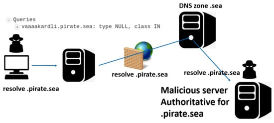 Figure 1. Path of DNS packets during a DNS proxy tunneling attack.
While the plaintext nature of DNS transmission aids in security inspections, it also presents significant privacy concerns. This has prompted the creation of secure protocols designed to protect DNS privacy, such as the DNS over HTTPS [9]. A solution to block this attack involves the use of firewalls implementing DNS packet inspection. However, this operation could not be allowed by the previously discussed encrypted DNS queries. Moreover, it is time-consuming and not suitable for firewall management of LANs composed of a high number of devices and a high volume of incoming and outgoing DNS packets. More practical strategies can be implemented to promptly detect this kind of attack and trigger proper countermeasures. As detailed in the next sections, the proposed solution does not require a deep packet inspection at the application layer; therefore, it addresses these issues.
3. Related Works
Multiple methods and approaches to detect DNS tunneling attacks have been proposed in the literature [10]. The most innovative and effective solutions employ ML algorithms to analyze DNS traffic from a statistical viewpoint, avoiding time-consuming packet inspection operations. These approaches can be grouped into four main families depending on how these approaches group packets to extract features: Per-transaction, Per-query, Per-domain, and Per-IP.
In the following subsections, we add some details about each of these families, the main papers in the literature describing methods belonging to each family, and the related considered features. Some of these features are referred to some fields of the DNS packets while others are defined ad hoc by the authors. Additional information useful for better understanding the features can be found in [8] and in the papers referenced hereinafter.
3.1. Per-Query Family
Per-query approaches try discovering tunnels by analyzing single FQDN queries, regardless of client/server interactions. These approaches consider some fields of every single DNS query and/or reply as input. The extracted features are usually related to properties of the string, such as the entropy, number and ratio of different types of characters, length, and so on.
The main papers describing per-query approaches, considered features, and used ML algorithms are reported in Table 1.

Table 1.
Papers proposing per-query detection approaches.
While per-query approaches generally show a very good performances in detecting attacks, they usually suffer from a high false-positive rate. The reason, as explained in the papers themselves, is that there are a lot of legitimate services based on DNSs, such as Content Delivery Networks, that produces queries that are very similar to the rogue ones.
3.2. Per-Transaction Family
ChatGPT ha detto:
Per-transaction methods aim to detect covert channels between client–server pairs by examining characteristics of their request/response exchanges. Each request/response pair is taken as input, organized by client and server IP addresses, and distinguished through the transaction ID: . They extract arrival timing information and/or some information from both query and reply fields. The extracted features allow the identification of compromised DNS communication. The features can subsequently be computed over every single transaction or over a set of transactions, for example in a specific time window.
The main papers describing Per-transaction approaches, considered features, and used ML algorithms are reported in Table 2.
Table 2.
Papers proposing per-transaction detection approaches.
Per-transaction approaches, thanks to the information related to the client–server interaction, partially solve the issue of false positives of per-query approaches. In particular, Ref. [15] shows very good performances in terms of specificity.
To the best of our knowledge, Ref. [19] is the only work that specifically addressed the issue of Explainability in DNS tunneling detection by using traditional supervised classification algorithms. The goal of our work is to make a neural network-based solution explainable, exploiting both the improved performances of neural networks in anomaly detection problems and explainable algorithms.
3.3. Per-IP Family
Per-IP methods analyze all packets generated by a particular IP address. The extracted features, primarily derived from timing information, are then used to detect a compromised client.
The main papers describing per-IP approaches, considered features, and used ML algorithms are reported in Table 3.
The main advantage of per-IP approaches is that they allow for precise detection of the compromised machine inside the network. From the other side, these detection methods can be easily tricked by simply decreasing the number of packets generated (at the cost of decreasing the bandwidth of the covert channel).
3.4. Per-Domain Family
Per-domain methods aggregate all DNS packets directed to a given second-level domain and derive features from these packet groups. Each group may consist of either a predefined number of packets or all packets captured within a specified time window. The resulting features are then used to detect whether the domain is compromised.
The main papers describing per-domain approaches, considered features, and used ML algorithms are reported in Table 4.
Table 3.
Papers proposing per-IP detection approaches.
Table 3.
Papers proposing per-IP detection approaches.
| Paper | Features | Algorithms | Dataset | Performance |
|---|---|---|---|---|
| [21] | Time interval between query and response (mean and variance), packet size (mean and variance), subdomain entropy (mean and variance of unigram, bigram, trigram entropy), record types (frequency of all 8 resource records) | Binary classification | Unknown | |
| [22] | Length of domain names (average), number of labels (average), number of different hostnames, length of hostnames (average), information entropy of hostnames, length of DNS messages (average), proportion of big upstream packets, proportion of small downstream packets, upload/download payload ratio | Decision Tree, Random Forest, K-NN, SVM | ≈11,000 packets |
Table 4.
Papers proposing per-domain detection approaches.
Table 4.
Papers proposing per-domain detection approaches.
| Paper | Features | Algorithms | Dataset | Performance |
|---|---|---|---|---|
| [23] | Character entropy, non-IP type ratio, unique query ratio and volume, rate of A and AAAA records, average query length, ratio between the length of the longest meaningful word and the subdomain length | Isolation Forest | ≈ packets | |
| [24] | Nameservers, domains and lowest-level subdomains character frequencies | Comparison between the character ranks and frequencies with Zipfian distribution of the English language | Unknown | Unknown |
| [25] | 29 features, including statistics over subdomains and record types | Isolation Forest | ≈250,000 domains |
Per-domain approaches show generally good performances, though they may suffer from a high false-positive rate due to legitimate services that produce strange patterns in DNS packets; despite these features, Ref. [23] show very good performances.
4. DNS Tunneling Detection
DNS tunneling detection can be seen as an example of an anomaly detection problem. It is a binary classification problem where the two classes represent the ‘absence’ (label 0) or ‘presence’ (label 1) of an anomaly (in this case, a tunneling attack). All the solutions mentioned in Section 3 involve employing ML algorithms to exploit traffic statistics extracted from DNS packets.
The selection of models in this study—autoencoders, decision trees, and logic learning machines (LLMs)—is motivated by both their technical suitability for anomaly detection and their compatibility with explainability objectives.
- Autoencoders are well-suited for modeling normal traffic patterns in an unsupervised manner. By learning a compact representation of benign DNS queries, the autoencoder can identify anomalies—such as those caused by tunneling—through elevated reconstruction errors. This makes it ideal for scenarios where labeled malicious data is scarce or evolving.
- Decision trees serve as an interpretable surrogate model to map the latent representations or reconstruction-based outputs of the autoencoder to symbolic rules. Their hierarchical structure is aligned with human reasoning, making the derived rules intuitive and easy to audit. Moreover, their fast inference capability supports real-time applications in network environments.
- Logic Learning Machines (LLMs) provide a symbolic learning framework based on the Switching Neural Network paradigm. Unlike traditional decision trees, LLMs generate flat IF–THEN rules that can offer more compact and generalizable representations. Their rule-based nature facilitates integration with intrusion detection systems and policy-based security controls.
These models were chosen to complement one another: the autoencoder acts as the anomaly detector, while the decision tree and LLM serve as interpretable layers that convert anomalies into human-readable logic. We also acknowledge the limitations of each model: autoencoders may overfit to noisy features; decision trees may suffer from instability due to data sparsity; and LLMs may require careful tuning to avoid rule bloat. Nevertheless, this combination provides a strong balance between detection performance and explainability, which is essential for practical deployment in cybersecurity operations.
With the following series of tests, we want to evaluate
- The performances of a widely used “black box” approach, such as the autoencoder.
- The performances of two different “white box” approaches (which are expected to be lower.
- The effectiveness of the combination of XAI and autoencoder as the best tradeoff between performances and explainability.
4.1. Datasets and Extracted Features
In order to test the proposed solution, we used the collection of DNS traffic from a large network, which comprises both legitimate traffic and rogue traffic. Regular traffic information was collected at CNR premises, IEIIT, Genova, Italy. We generated perfectly balanced datasets specifically to study the various overlaps of hidden traffic in DNS. The considered case of 10% of hidden traffic generates difficult instances of the binary supervised classification problem; namely, a significant number of illegitimate samples overlap with legitimate samples. Lower percentages lead to impossible detection and claims related to more complex approaches, such as majority voting over time. The following operations allow us to generate variations of the datasets. A mix of DNS (label 0 in the datasets) with tunnels (for ssh and p2p separately, label 1 in the datasets) is created. The approach can be generalized to any desired application compatible with the DNS2TCP tool. Different mixtures of hidden application inside regular DNSs are applicable: 50%, 10%, 1%, and 0.1%. Decreasing percentages increase the difficulty of the problem as hidden traffic becomes widely spread in time over legitimate DNS. Datasets and original traffic dumps from the network (raw data) are available from the GitHub repository [16].
In order to preserve the privacy of the users of the network, we decided to publish the features extracted from the packets, as detailed below. The dataset is available at [16]. To generate tunneled traffic, three applications are tunneled through the DNS2TCP tool [26]. As shown in [15], DNS2TCP, used in this paper, is the most silent tool in tunnel creation, compared to iodine or other tools. Therefore, we did not consider investigating other tools. We used three applications to generate both genuine and the malicious packets. The first one is a dump of an entire website, where tunneling is performed by using a proxy setting on and the DNS server forwards DNS packets to a squid proxy application. The second one is an protocol session, where tunneling is performed by executing simple commands through a connection directly executed from the rogue DNS server to a local host. The third one is a peer-to-peer (p2p) application, where tunneling has been set up by using proxy socks [15]. We denote the six sub-datasets of DNS packets generated by using these three applications with , and according to the absence or presence of a tunnel attack. For each application, we have 80,000 labeled 0 packets and 80,000 labeled 1 packets.
As input features, we consider the same information considered in [18] and described below. Table 5 shows the twelve features computed for each coupled DNS query–response packet considering three physical quantities (Q—size of the DNS query packet; A—size of the DNS response packet; and —time interval between a DNS query transmission and the related DNS response reception) and four different statistics per quantity (m—mean; v—variance; k—kurtosis; and s—skewness). Each array of twelve elements is a sample that belongs to one of the two classes. The rationale behind the choice of features has been discussed in detail in a previous paper. In brief, it has been noticed that, usually, DNS tunneling tools generate larger queries with irregular patterns over time; moreover, the response time of the rogue server hugely differs from the legitimate ones, particularly in the cases in which DNS tunneling is used as a proxy for internet traffic.
Table 5.
Features extracted from the DNS traffic.
Table 5.
Features extracted from the DNS traffic.
| Statistics—Physical Variables | Q | A | Dt |
|---|---|---|---|
| Mean | mQ | mA | mDt |
| Variance | vQ | vA | vDt |
| Kurtosis | kQ | kA | kDt |
| Skewness | sQ | sA | sDt |
4.2. Autoencoder-Based “Black-Box” Method
We first consider an autoencoder-based “black-box” solution to detect the DNS tunnels. Its operational steps are summarized in Figure 2.
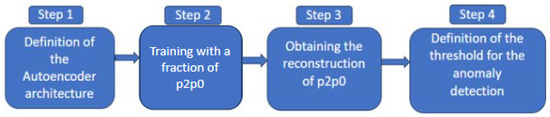
Figure 2.
Operational steps of the Autoencoder-based method.
4.2.1. Step 1—Definition of the Autoencoder Architecture
Autoencoders are neural network-based models whose aim is to reconstruct the input by using the most meaningful features obtained through a dimensional reduction in the latent space [27,28]. The typical architecture () is composed of encoder and decoder parts, where the layers progressively reduce their dimensions, until the layer reaches the lower dimension, and then progressively increase them again. However, the accuracy of the autoencoder architecture is typically low in cases in which the samples of the two classes are very close within the feature space, as is the case for the dataset. The reason is that the initial twelve features do not contain enough information to produce new informative data in the latent space.
Since the initial twelve features do not contain enough information to produce new informative data in the latent space, the main idea behind the considered autoencoder architecture is to move to a higher-dimensional space before moving to the original lower-dimensional space. Therefore, with respect to traditional autoencoder architectures, the proposed solution involves a more complex architecture.
The autoencoder is composed of six hidden layers, with the following dimensions Table 6:
Table 6.
Autoencoder architecture.
The considered autoencoder settings are the ReLu activation function for each hidden layer, Sigmoid function for the output layer, LogCosh loss function, and Adam optimizer.
This architecture is shown in Figure 3 where, for the sake of visualization, the number of neurons of each layer has been divided by six.
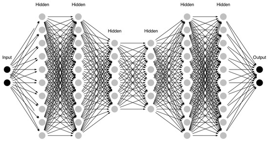
Figure 3.
Logical scheme of the considered autoencoder architecture.
4.2.2. Step 2—Training with and Step 3—Obtaining the Reconstruction of
After the definition of the autoencoder architecture, we train the model by using one of the three genuine sub-datasets (the one defined as ) in order to keep the others for the tests. Due to the nature of the autoencoder, we obtain the reconstruction of , denoted as . The differences between the reconstruction and the original are fundamental for the definition of the autoencoder threshold.
4.2.3. Step 4—Definition of the Threshold for the Anomaly Detection
We compute the histogram of the Mean Absolute Error between and and define the autoencoder error threshold as
where and are the mean and variance, respectively, computed over all the samples of .
The threshold is defined by evaluating the reconstruction error of the training dataset; in particular, we set the value that would limit the false positives in the training dataset to below 99%.
After defining the threshold , we can classify any input data as anomalous or not by following the two steps listed below:
- Compute the Mean Absolute Error between an input sample s and its reconstructed counterpart r.
- Check with the threshold : the anomaly occurs whenever .
Thus, a new label (0-genuine or 1-tunnel) is inferred for each sample passed as input to the autoencoder, obtaining six other sub-datasets denoted as , , and .
4.3. XAI-Based “White-Box” Method
Most of the approaches mentioned in Section 3 are based on “black-box” solutions that are able to achieve a good performance without allowing users to understand how the obtained results have been achieved. In addition, in case of particular needs, such as the minimization of the false-positive rate (FPR), “black-box” approaches do not allow users to manually adjust rules or clearly see which of the features could be the ones to focus on to achieve the performance target.
XAI can help us to achieve this objective. Cybersecurity systems are among the scenarios where XAI has been suggested for multiple purposes, including—but not limited to—anomaly detection [29,30]. Rule-based models, such as LLM [31,32] and DT [33], usually expressed as decision rules in the IF–THEN form, have been proven to be examples of transparent-by-design, global, model-specific techniques for cybersecurity.
For this reason, after addressing the problem by using a “black-box” approach, we attempt to make it explainable through the use of a ruleset in the IF–THEN format [34]. We obtain this ruleset by using both DT and LLM, where LLM is a global, transparent by-design model developed as a computational improvement of Switching Neural Networks (SNNs) [31] by using the software Rulex (https://www.rulex.ai (accessed on 5 June 2025)). We chose to employ both DT and LLM due to their complementary working principles. DT operates by evaluating the discriminative power of individual features, whereas LLM generates rules through a three-stage process: first, the feature space is discretized and binarized using inverse-only-one coding; next, the resulting binary strings are concatenated into a single long string representing the samples; and finally, shadow clustering is applied to construct logical structures, known as implicants, which are then converted into simple conditions and combined into a set of interpretable rules [34].
Since we need both genuine and tunnel samples to generate a set of rules by using DT and LLM, we consider three different scenarios as outlined in Figure 4.
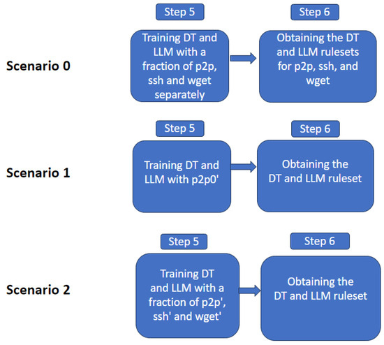
Figure 4.
Operational steps of the XAI-based method.
- Scenario 0—Supervised XAI (S-XAI): DT and LLM are trained by using 70% of the three sub-datasets , , and separately in order to provide advances knowledge of all the anomalies indicated in the original dataset. In this way, we train three different DTs and LLMs according to the dataset to obtain the set of rules that characterize each application.
- Scenario 1—Unsupervised XAI (U-XAI): DTs and LLMs are trained by using only . In this way, the XAI algorithms are trained with only good data, and behave as pure anomaly detection algorithms.
- Scenario 2—Semi-supervised XAI (SS-XAI): DT and LLM are trained by using 70% of three sub-datasets , , and . Therefore, the anomalies detected by the autoencoders are used as labeled data for the training of XAI algorithms. In this way, the XAI algorithms learn to reproduce the behavior of the autoencoder in terms of classification, but based on explainable rules.
In this way, we have a totally supervised solution in Scenario 0 (supervised eXplainability), a completely unsupervised solution in Scenario 1 (unsupervised autoencoder and unsupervised eXplainability), and a semi-supervised solution in Scenario 2 (unsupervised autoencoder and supervised eXplainability).
4.4. Feature Ranking and Rule Confidence
From the knowledge extraction perspective, it is possible to inspect rule structures through feature ranking and rule confidence.
Consider a set of m rules , each including conditions . Also, let be the class assigned by the k-th rule and be the real output of the j-th instance.
A condition involving a variable can assume one of the following forms:
being s, t∈.
Each rule produced by the algorithm can be represented by its own corresponding confusion matrix. The indices that comprise the matrix are and , defined as the number of instances that satisfy all the conditions in rule with and , respectively; and , defined as the number of examples which do not satisfy at least one condition in rule , with and , respectively.
Therefore, the following metrics can be obtained [35]:
The covering is adopted as a measure of relevance for a rule ; as a matter of fact, the greater the covering, the higher the generality of the corresponding rule. The error is a measure of how many data are wrongly covered by the rule. Both covering and error are used to define feature ranking and the subsequent value ranking. The covering is used as an indicator of the relevance of a rule ; in practice, a larger covering implies that the rule is more general. The error represents the proportion of data incorrectly classified or covered by the rule. Together, covering and error serve as the basis for establishing feature ranking, followed by value ranking.
Feature ranking (FR) evaluates which features most strongly influence classification based on a relevance measure. To compute such measure of relevance for a condition, we consider the rule , in which the condition occurs, and the same rule where the condition does not occur, denoted as . Given that the premise part of is less stringent, we determine that ; thus, the quantity can be used as a measure of relevance for the condition of interest . Each condition is related to a specific variable and a measure of relevance , as it can be derived through the Equation (5):
where the product is computed based on the rules that include a condition for the variable of interest. This measure varies in . The same concept, but restricted to specific intervals of the variables, gives rise to Value Ranking (VR).
Moreover, any condition defines a domain in the input space corresponding to an interval for feature . Let for each j and be the set of rules of class l. A score with every class l is then defined as
and every input (i.e., feature vector) I is assigned to the class with the largest score with rule confidence given by
where and are the first and second largest scores, respectively. Such confidence represents how significantly the choice of the first class varies compared to the other candidate class. Large confidence (on a given input) means the model decision (for classification of that input) is trustable. Small confidence means the model is not so certain of the decision and the user is made aware of this.
5. Performance Evaluation
We measure and compare the obtained performance in terms of the true-positive rate (TPR) and true-negative rate (TNR):
where is the number of positive (1) samples correctly classified as positive (true positive), is the number of positive samples wrongly classified as negative (false negative), is the number of negative (0) samples correctly classified as negative (true negative), and is the number of negative samples wrongly classified as positive (false positive).
5.1. Autoencoder Results
The first set of tests has been performed to assess the autoencoder-based solution. Figure 5 shows the obtained histogram and the error threshold computed by using Equation (1), while Figure 6 shows the overall error and points out the reconstruction precision of the samples.
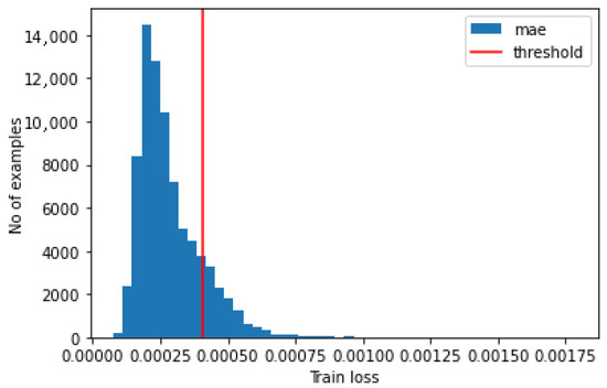
Figure 5.
Autoencoder: histogram.
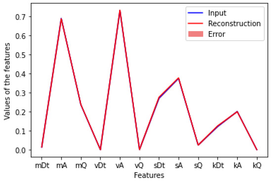
Figure 6.
Autoencoder: Reconstruction error.
Table 7 shows the obtained performance results separated for the three considered applications.
Table 7.
Autoencoder: TPR and TNR performance.
The autoencoder-based solution works well in all the considered cases, even though there is a slight overfit for the and cases, which is also visible looking at the ROC curves shown in Figure 7, where the false-positive rate (FPR) is defined as
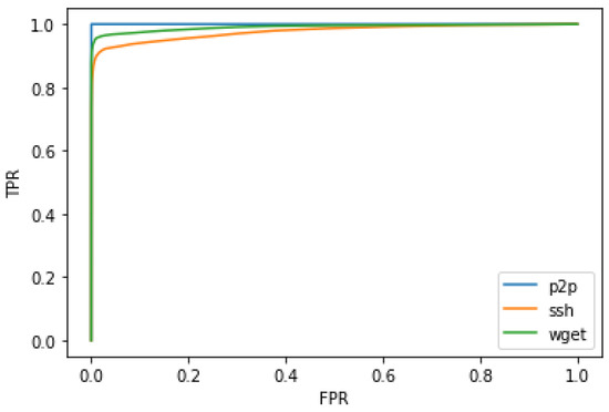
Figure 7.
Autoencoder: ROC curves.
5.2. Supervised-XAI Results
The second set of tests has been performed to assess the XAI-based solution in the supervised configuration (S-XAI - Scenario 0). Different sets of rules have been extrapolated by using DT and LLM and separately considering , , and sub-datasets.
By using DT, we extrapolate 14 rules in the case and, as expected due to their higher complexity, 350 and 217 rules in the and cases, respectively. Table 8 shows the obtained performance results separated for the three considered applications.
Table 8.
S-XAI using DT: TPR and TNR performance.
By using an LLM, we extrapolate a smaller number of rules (10, 105, and 60 rules for the , , and applications, respectively), and it achieves a worse performance, as shown in Table 9.
Table 9.
S-XAI using LLM: TPR and TNR performance.
For all the cases, we also rank the features from the most useful for detection to the least useful one in order to understand which features offer the greatest contribution to the tunnel/non-tunnel discrimination. Feature ranking assigns to each feature a number within the range [0,1] representing its importance to produce the rules. This value is obtained through a sensitivity analysis of both the covering and the error of the features [32]. Since DT exhibits a better performance than LLM in all of the considered cases, we show only the feature ranking obtained using DT in the three considered scenarios.
Table 10 shows the feature ranking by using DT for each application.
Table 10.
S-XAI by using DT: Feature ranking.
5.3. Unsupervised-XAI Results
The third set of tests has been performed to assess the XAI-based solution in the unsupervised configuration (U-XAI—Scenario 1).
By using DT, we extrapolated 409 rules and obtained the performance results shown in Table 11.
Table 11.
U-XAI by using DT: TPR and TNR performance.
By using LLM, we extrapolated 30 rules and obtained the performance results shown in Table 12.
Table 12.
U-XAI by using LLM: TPR and TNR performance.
5.4. Semi-Supervised-XAI Results
The fourth set of tests has been performed to assess the XAI-based solution in the semi-supervised configuration (SS-XAI—Scenario 2).
By using DT, we extrapolated 648 rules and obtained the performance results shown in Table 13.
Table 13.
SS-XAI using DT: TPR and TNR performance.
By using LLM, we extrapolated 29 rules and obtained the performance results shown in Table 14.
Table 14.
SS-XAI using LLM: TPR and TNR performance.
Since we have trained the DT and LLM on a single dataset in both U-XAI and SS-XAI configurations, we have a unique set of rules and, consequently, a unique feature ranking, as shown in Table 15.
Table 15.
U-XAI and SS-XAI using DT: Feature ranking.
To show an example of the rules obtained by our proposed approach, we report the three most meaningful rules for each dataset, where denotes the covering rate of each rule:
- if mQ > 0.252609 and 0.020092 < sQ ≤ 0.509763 and vQ ≤ 0.623669 then 1 ()
- if mQ ≤ 0.252609 and sQ ≤ 0.061033 then 0 ()
- if mQ ≤ 0.252609 and sQ > 0.257355 then 0 ()
- if sA ≤ 0.206723 and vA ≤ 0.497214 then 1 ()
- if sA > 0.296982 and sQ ≤ 0.039690 and mA ≤ 0.422886 and vQ > 0.001981 and kQ ≤ 0.366810 then 0 ()
- if sA > 0.261134 and sQ > 0.060930 and vQ ≤ 0.015255 then 1 ()
- 1.
- if sA > 0.342 and mA ≤ 0.460 then 0 ()
- 2.
- if sA ≤ 0.227 and vA ≤ 0.434 then 0 ()
- 3.
- if sA ≤ 0.189 and 0.434 ≤ vA ≤ 0.525 then 1 ()
The XAI rules can be used to motivate the decision of the algorithm. Considering, for example, Rule 1 of the dataset, we know that DNS queries containing tunnels are usually longer than normal queries, with some exceptions (such as Content Delivery networks). The rule decides for the tunnel if , which means the queries are longer than a certain threshold, and and , which means that a high percentage of queries have a significant length, which is unusual for legitimate services. This rule is sufficient to discriminate between the two classes in of the cases, helping the network engineer to look for the related DNS server and eventually block it properly by configuring the firewall.
Figure 8 and Figure 9 show the confidence of correct and incorrect classifications of SSH, respectively, where the left and right portions of each figure are related to legitimate and tunnel traffic, respectively. As expected, large confidence values are achieved under correct detection. Though partially overlapping (some values in the left part of Figure 9 (wrong) are larger than 0.2, which is the minimum in Figure 8 (correct)), the largest part of the cases highlight the separation between correct and wrong cases through confidence. In other words, incorrect detections are associated with low or very low confidence. According to Equation (7), incorrect samples are characterized by the close proximity of candidate classes with respect to the correct ones. The confidence thus is revealed to be a reliable indication of model trust.
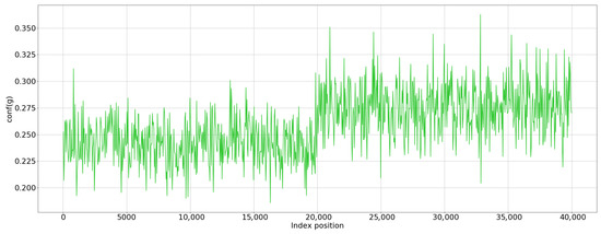
Figure 8.
Confidence of correct classifications.
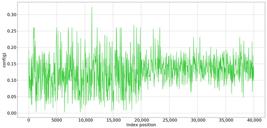
Figure 9.
Confidence of incorrect classifications.
5.5. Results and Discussion
As expected, the autoencoder-based solution works well on all the datasets (see Table 7), but it does not provide any understandable information to allow the users to understand their choices. On the other hand, the XAI-based method offers this kind of information, showing the rule sets and ranking the features depending on their importance, but the obtained performance is not satisfying for all three of the considered configurations.
S-XAI performs as well as the autoencoder (in some cases even better; see Table 8 and Table 9), but it does not use the results of the autoencoder as input. This configuration can be used instead of the autoencoder, but not to make it explainable.
In the unsupervised configuration, the introduction of the eXplainability does not allow the autoencoder to be made explainable without a significant performance decrease (see Table 11 and Table 12). The obtained TPR is low, which means that most of the anomalies are not well detected. The main reason is that the 0 and 1 classes are completely imbalanced. In fact, since the autoencoder works quite well, almost all the reconstructed are classified with label 0.
A better solution for the considered problem is represented by the semi-supervised configuration, whose obtained performance (see Table 13 and Table 14) shows how it can allow a good trade-off to be achieved between TPR and TNR. The 0 and 1 classes are now balanced, making the obtained accuracy high enough to allow one to rely solely on the extrapolated rules to perform the classification of the anomalies.
In all cases, LLM allows a smaller rule set to be obtained, and consequently, less time is needed to perform the classification, at the cost of a small performance decrease. In addition, the classification of samples requires a smaller number of features than and . When the number of rules is too small, each rule must cover broader behavior in the data. This may lead to generalized conditions that may be hard to interpret or verify and loss of fidelity to the actual behavior of the underlying model. In contrast, a larger number of rules often breaks down the logic into more specific, easier-to-understand segments. Overall, an excessively small number of rules tends to generalize too much, making them harder to explain, harder to map to real-world concepts, and less reliable when generalizing or extrapolating to unseen data.
Finally, the feature rankings reported in Table 10 and Table 15 allow us to notice that some features are significant in all cases. For example, is the most significant for S-XAI and the second most significant for S-XAI , S-XAI , and SS-XAI.
One of the main problems associated with the practical implementation of IDS is the false-positive rate; an excessive number of alarms cannot be managed by human operators in Security Operation Centers. The rules can be used to “retouch” the algorithm on the specific network. For example, based on the rules described above, it can be noticed that, in this specific network, mQ (the mean length of the query) is a particularly significant feature; this means that if it is possible to "whitelist" some specific domains, it is possible to increase the performance.
While this study focuses on DNS tunneling detection, the proposed rule-based eXplainable Autoencoder framework has the potential to be generalized to other types of network-based attacks, such as Distributed Denial of Service attacks or malware propagation. These threats, like DNS tunneling, often exhibit anomalous patterns that can be captured by an autoencoder and translated into interpretable rule sets. However, such generalization requires careful consideration of the input feature space, since the features relevant for DNS tunneling may not be directly transferable to other scenarios. As a result, while the XAI results in this study are promising, further research is needed to evaluate the robustness and adaptability of the approach across different threat types. In particular, future studies should investigate how changes in feature representation affect the learned rules and their interpretability, as this has a direct impact on the model’s effectiveness and transparency in diverse security contexts.
6. Conclusions
This paper proposed an approach to anomaly detection problems in network monitoring, specifically DNS tunneling detection, and showed how the considered XAI models (DT and LLM) can be successfully used, if properly configured, to make the classical “black-box" approaches, such as the considered autoencoder-based method, explainable. This study details the configuration of the XAI-based approach that is used to obtain performance results comparable with the autoencoder-based approach, and also highlights the main discriminant features that are used to carry out anomaly detection. Even if the XAI model produces a small decrease in performance, in a practical implementation, the explainable approach can significantly facilitate the work of network engineers and security operation center analysts, resulting in a more rapid and efficient attack response. Therefore, this study is a step forward toward the large-scale use of explainable models in cybersecurity monitoring systems. Before the adoption of the proposed approach in real infrastructures, two main improvements would be useful: on one hand, in future works, we will implement new tests to check if the proposed approach produces rules that are robust against variations in the monitored network over time; also, it will be interesting to test the applicability of explainable models to multiple network monitoring scenarios, so as to implement explainability over a large set of monitoring algorithms.
Author Contributions
Conceptualization, M.M. (Maurizio Mongelli); methodology, M.M. (Maurizio Mongelli); software, G.D.B.; validation, G.B.G. and F.P.; investigation, G.D.B.; resources, M.M. (Maurizio Mongelli); data curation, M.M. (Maurizio Mongelli) and G.D.B.; writing—original draft preparation, G.D.B., G.B.G. and F.P.; writing—review and editing, G.D.B., G.B.G. and F.P.; supervision, F.P., S.Z., M.M. (Mario Marchese) and M.M. (Maurizio Mongelli); project administration, F.P. and M.M. (Maurizio Mongelli); funding acquisition, F.P., M.M.(Mario Marchese) and M.M. (Maurizio Mongelli). All authors have read and agreed to the published version of the manuscript.
Funding
The work was developed under Future Artificial Intelligence Research (FAIR) project, Italian Recovery and Resilience Plan (PNRR), Spoke 3—Resilient AI.
Data Availability Statement
The dataset has been published in [16].
Conflicts of Interest
The authors declare no conflicts of interest.
Abbreviations
The following abbreviations are used in this manuscript:
| AI | Artificial Intelligence |
| ML | Machine Learning |
| DNS | Domain Name System |
| XAI | eXplainable AI |
| DT | Decision Tree |
| LLM | Logic Learning Machine |
| U-XAI | Unsupervised eXplainable Artificial Intelligence |
| SS-XAI | Semi-Supervised eXplainable Artificial Intelligence |
| MAE | Mean Absolute Error |
References
- Alsajri, A.; Steiti, A. Intrusion Detection System Based on Machine Learning Algorithms:(SVM and Genetic Algorithm). Babylon. J. Mach. Learn. 2024, 2024, 15–29. [Google Scholar] [CrossRef]
- Zhang, J.; Qian, K.; Luo, H.; Liu, Y.; Qiao, X.; Xu, X.; Tian, J. Process monitoring for tower pumping units under variable operational conditions: From an integrated multitasking perspective. Control Eng. Pract. 2025, 156, 106229. [Google Scholar] [CrossRef]
- Zhang, J.; Tian, J.; Yan, P.; Wu, S.; Luo, H.; Yin, S. Multi-hop graph pooling adversarial network for cross-domain remaining useful life prediction: A distributed federated learning perspective. Reliab. Eng. Syst. Saf. 2024, 244, 109950. [Google Scholar] [CrossRef]
- Xu, F.; Uszkoreit, H.; Du, Y.; Fan, W.; Zhao, D.; Zhu, J. Explainable AI: A brief survey on history, research areas, approaches and challenges. In Proceedings of the International Conference on Natural Language Processing and Chinese Computing (NLPCC), Dunhuang, China, 9–14 October 2019; Springer: Berlin/Heidelberg, Germany, 2019; pp. 563–574. [Google Scholar]
- Narteni, S.; Orani, V.; Cambiaso, E.; Rucco, M.; Mongelli, M. On the Intersection of Explainable and Reliable AI for physical fatigue prediction. IEEE Access 2022, 10, 76243–76260. [Google Scholar] [CrossRef]
- Graziani, M.; Dutkiewicz, L.; Calvaresi, D.; Amorim, J.P.; Yordanova, K.; Vered, M.; Nair, R.; Abreu, P.H.; Blanke, T.; Pulignano, V.; et al. A global taxonomy of interpretable AI: Unifying the terminology for the technical and social sciences. Artif. Intell. Rev. 2023, 56, 3473–3504. [Google Scholar] [CrossRef]
- Loyola-Gonzalez, O. Black-box vs. white-box: Understanding their advantages and weaknesses from a practical point of view. IEEE Access 2019, 7, 154096–154113. [Google Scholar] [CrossRef]
- Mockapetris, P.V. RFC1035: Domain Names-Implementation and Specification. 1987. Available online: https://datatracker.ietf.org/doc/html/rfc1035 (accessed on 5 June 2025).
- Zhan, M.; Li, Y.; Yu, G.; Li, B.; Wang, W. Detecting DNS over HTTPS based data exfiltration. Comput. Netw. 2022, 209, 108919. [Google Scholar] [CrossRef]
- Wang, Y.; Zhou, A.; Liao, S.; Zheng, R.; Hu, R.; Zhang, L. A comprehensive survey on DNS tunnel detection. Comput. Netw. 2021, 197, 108322. [Google Scholar] [CrossRef]
- Ahmed, J.; Gharakheili, H.H.; Raza, Q.; Russell, C.; Sivaraman, V. Monitoring Enterprise DNS Queries for Detecting Data Exfiltration from Internal Hosts. IEEE Trans. Netw. Serv. Manag. 2020, 17, 265–279. [Google Scholar] [CrossRef]
- Sammour, M.; Hussin, B.; Othman, M.F.I. Comparative Analysis for Detecting DNS Tunneling Using Machine Learning Techniques. Int. J. Appl. Eng. Res. 2017, 12, 12762–12766. [Google Scholar]
- Das, A.; Shen, M.Y.; Shashanka, M.; Wang, J. Detection of exfiltration and tunneling over DNS. In Proceedings of the International Conference on Machine Learning and Applications (ICMLA), Cancun, Mexico, 18–21 December 2017; pp. 737–742. [Google Scholar]
- Wu, K.; Zhang, Y.; Yin, T. FTPB: A Three-stage DNS Tunnel Detection Method Based on Character Feature Extraction. In Proceedings of the International Conference on Trust, Security and Privacy in Computing and Communications (TrustCom), Guangzhou, China, 29 December 2020–1 January 2021; pp. 250–258. [Google Scholar]
- Aiello, M.; Mongelli, M.; Papaleo, G. DNS tunneling detection through statistical fingerprints of protocol messages and machine learning. Int. J. Commun. Syst. 2015, 28, 1987–2002. [Google Scholar] [CrossRef]
- Open Data of DNS Tunneling. 2024. Available online: https://github.com/mopamopa/DNS-tunneling (accessed on 5 June 2025).
- Cambiaso, E.; Aiello, M.; Mongelli, M.; Papaleo, G. Feature transformation and Mutual Information for DNS tunneling analysis. In Proceedings of the International Conference on Ubiquitous and Future Networks (ICUFN), Vienna, Austria, 5–8 July 2016; pp. 957–959. [Google Scholar]
- Aiello, M.; Mongelli, M.; Muselli, M.; Verda, D. Unsupervised learning and rule extraction for Domain Name Server tunneling detection. Internet Technol. Lett. 2019, 2, 1–6. [Google Scholar] [CrossRef]
- Zebin, T.; Rezvy, S.; Luo, Y. An explainable AI-based intrusion detection system for DNS over HTTPS (DoH) attacks. IEEE Trans. Inf. Forensics Secur. 2022, 17, 2339–2349. [Google Scholar] [CrossRef]
- CIRA-CIC-DoHBrw-2020. 2020. Available online: https://github.com/doh-traffic-dataset/CIRA-CIC-DoHBrw-2020-and-DoH-Tunnel-Traffic-HKD (accessed on 5 June 2025).
- Liu, J.; Li, S.; Zhang, Y.; Xiao, J.; Chang, P.; Peng, C. Detecting DNS tunnel through binary-classification based on behavior features. In Proceedings of the Trustcom/BigDataSE/ICESS, Sydney, NSW, Australia, 1–4 August 2017; pp. 339–346. [Google Scholar]
- Yang, Z.; Hongzhi, Y.; Lingzi, L.; Cheng, H.; Tao, Z. Detecting DNS Tunnels Using Session Behavior and Random Forest Method. In Proceedings of the International Conference on Data Science in Cyberspace (DSC), Hong Kong, China, 27–30 July 2020; pp. 45–52. [Google Scholar]
- Nadler, A.; Aminov, A.; Shabtai, A. Detection of malicious and low throughput data exfiltration over the DNS protocol. Comput. Secur. 2019, 80, 36–53. [Google Scholar] [CrossRef]
- Born, K.; Gustafson, D. Detecting DNS tunnels using character frequency analysis. arXiv 2010, arXiv:1004.4358. [Google Scholar] [CrossRef]
- Luo, M.; Wang, Q.; Yao, Y.; Wang, X.; Yang, P.; Jiang, Z. Towards Comprehensive Detection of DNS Tunnels. In Proceedings of the Symposium on Computers and Communications (ISCC), Rennes, France, 7–10 July 2020; pp. 1–7. [Google Scholar]
- Dns2tcp. 2017. Available online: https://github.com/alex-sector/dns2tcp (accessed on 5 June 2025).
- Bank, D.; Koenigstein, N.; Giryes, R. Autoencoders. In Machine Learning for Data Science Handbook: Data Mining and Knowledge Discovery Handbook; Springer: Berlin/Heidelberg, Germany, 2023; pp. 353–374. [Google Scholar]
- Michelucci, U. An introduction to autoencoders. arXiv 2022, arXiv:2201.03898. [Google Scholar] [CrossRef]
- Capuano, N.; Fenza, G.; Loia, V.; Stanzione, C. Explainable Artificial Intelligence in CyberSecurity: A Survey. IEEE Access 2022, 10, 93575–93600. [Google Scholar] [CrossRef]
- Zhang, Z.; Al Hamadi, H.; Damiani, E.; Yeun, C.Y.; Taher, F. Explainable artificial intelligence applications in cyber security: State-of-the-art in research. IEEE Access 2022, 10, 93104–93139. [Google Scholar] [CrossRef]
- Muselli, M. Switching neural networks: A new connectionist model for classification. In Proceedings of the Italian Workshop on Neural Nets (WIRN) and International Workshop on Natural and Artificial Immune Systems (NAIS), Vietri sul Mare, Italy, 8–11 June 2005; Springer: Berlin/Heidelberg, Germany, 2006; pp. 23–30. [Google Scholar]
- Parodi, S.; Filiberti, R.; Marroni, P.; Libener, R.; Ivaldi, G.P.; Mussap, M.; Ferrari, E.; Manneschi, C.; Montani, E.; Muselli, M. Differential diagnosis of pleural mesothelioma using Logic Learning Machine. BMC Bioinform. 2015, 16, S3. [Google Scholar] [CrossRef]
- James, G.; Witten, D.; Hastie, T.; Tibshirani, R.; James, G.; Witten, D.; Hastie, T.; Tibshirani, R. Statistical learning. In An Introduction to Statistical Learning: With Applications in R; Springer: Berlin/Heidelberg, Germany, 2021; pp. 15–57. [Google Scholar]
- Narteni, S.; Orani, V.; Vaccari, I.; Cambiaso, E.; Mongelli, M. Sensitivity of Logic Learning Machine for Reliability in Safety-Critical Systems. IEEE Intell. Syst. 2022, 37, 66–74. [Google Scholar] [CrossRef]
- Cangelosi, D.; Blengio, F.; Versteeg, R.; Eggert, A.; Garaventa, A.; Gambini, C.; Conte, M.; Eva, A.; Muselli, M.; Varesio, L. Logic Learning Machine creates explicit and stable rules stratifying neuroblastoma patients. BMC Bioinform. 2013, 14, S12. [Google Scholar] [CrossRef]
Disclaimer/Publisher’s Note: The statements, opinions and data contained in all publications are solely those of the individual author(s) and contributor(s) and not of MDPI and/or the editor(s). MDPI and/or the editor(s) disclaim responsibility for any injury to people or property resulting from any ideas, methods, instructions or products referred to in the content. |
© 2025 by the authors. Licensee MDPI, Basel, Switzerland. This article is an open access article distributed under the terms and conditions of the Creative Commons Attribution (CC BY) license (https://creativecommons.org/licenses/by/4.0/).