Abstract
Real-time wildlife monitoring on edge devices poses significant challenges due to limited power, constrained bandwidth, and unreliable connectivity, especially in remote natural habitats. Conventional object detection systems often transmit redundant data of the same animals detected across multiple consecutive frames as a part of a single event, resulting in increased power consumption and inefficient bandwidth usage. Furthermore, maintaining consistent animal identities in the wild is difficult due to occlusions, variable lighting, and complex environments. In this study, we propose a lightweight hybrid tracking framework built on the YOLOv8m deep neural network, combining motion-based Kalman filtering with Local Binary Pattern (LBP) similarity for appearance-based re-identification using texture and color features. To handle ambiguous cases, we further incorporate Hue-Saturation-Value (HSV) color space similarity. This approach enhances identity consistency across frames while reducing redundant transmissions. The framework is optimized for real-time deployment on edge platforms such as NVIDIA Jetson Orin Nano and Raspberry Pi 5. We evaluate our method against state-of-the-art trackers using event-based metrics such as MOTA, HOTA, and IDF1, with a focus on detected animals occlusion handling, trajectory analysis, and counting during both day and night. Our approach significantly enhances tracking robustness, reduces ID switches, and provides more accurate detection and counting compared to existing methods. When transmitting time-series data and detected frames, it achieves up to 99.87% bandwidth savings and 99.67% power reduction, making it highly suitable for edge-based wildlife monitoring in resource-constrained environments.
1. Introduction
Wildlife monitoring is essential to understand animal behavior [1], track endangered species, manage human-wildlife conflict [2], and inform conservation strategies. In an era where biodiversity is constantly threatened by habitat loss, climate change, and poaching, timely and accurate data on animal populations has become more critical than ever. However, collecting these data in vast, remote, and often harsh environments is a major challenge. Traditional methods like manual observation or centralized video processing are labor-intensive, prone to error, or impractical for long-term deployment in the field [3].
Recent advances in artificial intelligence (AI), especially in the field of deep learning, have demonstrated great promise in improving wildlife monitoring efforts. By running intelligent models directly on edge devices, compact, low-power systems placed near the data source, we can perform real-time analysis of wildlife activity without relying on continuous network connectivity or cloud processing. YOLO (You Only Look Once), a state-of-the-art object detector [4,5,6,7], stands out as a perfect fit for this task due to its speed, accuracy, and efficiency on edge hardware. It enables fast animal detection in complex environments, making it possible to identify species and behaviors as they happen, even in the most remote locations.
Wildlife-monitoring systems rely heavily on centralized processing, where continuous video feeds or detection outputs are streamed from edge devices to central servers. These approaches, while effective in controlled environments, pose significant challenges in remote or resource-constrained settings. High bandwidth requirements, unreliable network connectivity, and increased power consumption make such systems impractical for long-term wildlife surveillance in the field.
In conventional detection-only systems, every frame is processed independently [8]. For example, consider a scenario where two identical animals are continuously moving within the field of view (FOV) of a camera for 10 s at a frame rate of 30 frames per second (FPS). This results in 300 frames, each detecting the same two animals, generating 600 redundant detection records that would typically be sent to the server [9]. This approach not only wastes bandwidth and energy but also leads to inefficiencies in data storage and animal counting, since there is no understanding of temporal continuity or object identity.
While some systems integrate tracking to reduce redundancy, traditional tracking algorithms are often limited. Many are sensitive to occlusions, lighting changes, or partial visibility, and they typically depend on either motion prediction or simple feature matching. These methods fail in real-world wildlife scenarios where animals may overlap, hide behind vegetation, or move under varied lighting conditions.
To overcome these challenges, we propose a hybrid tracking framework specifically designed for edge AI-based wildlife monitoring. Our system integrates the YOLO object detector for fast and accurate initial detection on edge devices with a Kalman filter-based motion tracker to maintain the position of animals over time. However, since the Kalman filter alone cannot handle visual appearance changes, such as similar-looking animals or those affected by occlusion or illumination, we incorporate Local Binary Patterns (LBPs) [10] and Hue, Saturation, and Value (HSV) [11] histograms as appearance-based features to enhance identity preservation. This hybrid approach significantly reduces the amount of data transmitted to the central server. In the previous example, instead of sending 600 detections over 10 s, our tracking system can assign consistent track_IDs to each animal and transmit only the time-series data associated with those unique IDs. This allows the edge device to send a single, meaningful record per tracked object, drastically reducing network load while maintaining high accuracy in detection and counting. Moreover, animal counting based solely on detection (frame-by-frame visibility) is inherently flawed, as it does not account for re-identification of the same animal across frames. Our proposed tracking-enhanced pipeline addresses this by maintaining consistent identity across time, ensuring accurate counts, and reducing false positives.
In a nutshell, the main contributions of our work are twofold:
- Lightweight and Robust Tracking Algorithm for Challenging Real-World Conditions: We propose a lightweight hybrid tracking algorithm that outperforms state-of-the-art methods such as ByteTrack and BoT-SORT across standard MOT metrics (MOTA, HOTA, IDF1), offering enhanced trajectory consistency and improved occlusion handling. The framework is evaluated on real-world wildlife footage captured under both day and night conditions. On particularly challenging nighttime wild boar sequences, it improves IDF1 by 57.8% (from 0.45 to 0.71), increases MOTA (from 0.58 to 0.60), and achieves the lowest number of false negatives (FN = 155). For wolf tracking, it matches top-performing trackers in daytime conditions (MOTA = 1.00, IDF1 = 1.00) and maintains strong performance at night (IDF1 = 0.95). Overall, the proposed approach delivers accurate and consistent tracking under complex environmental conditions.
- Edge-Optimized and Energy-Efficient Design: The hybrid tracking framework is optimized for deployment on edge devices such as the NVIDIA Jetson Orin Nano and Raspberry Pi 5. Our system achieves up to 99.87% power reduction (from 26.1 W to 0.05 W) and 99.67% bandwidth savings (from 168 Mbps to 0.57 Mbps) by minimizing redundant time-series data and frame transmissions.
Overall, these contributions enable real-time, energy-efficient, and reliable wildlife monitoring in bandwidth-constrained environments.
The remaining paper is structured as follows: Section 2 presents the necessary background knowledge and reviews related work in the field of object tracking. Section 3 details the materials and methods used in our study, while Section 4 specifically introduces our proposed hybrid tracking algorithm. The experimental evaluation metrics are thoroughly explained in Section 5, followed by a comprehensive analysis of the results comparing all trackers in Section 6. Finally, Section 7 concludes the paper with a summary of our findings and suggests promising directions for future research in wildlife tracking systems. This logical progression from foundational concepts to implementation and evaluation provides a complete framework for understanding our contributions to the field.
2. Related Works
The primary goal in detecting and tracking animals within the FOV of a camera is to accurately identify and follow their movements consistently, especially during rapid motion or positional changes. Achieving reliable tracking in such dynamic environments requires robust motion prediction mechanisms. In this context, the Kalman filter plays a vital role in enabling the prediction of an animal’s future position based on its current trajectory. This enhances tracking continuity and reduces identity switches, particularly beneficial when detections are intermittent or occluded.
Recent advances, such as in [12], DynaNet integrate traditional Kalman filtering with data-driven learning to improve motion modeling for autonomous vehicles. Similarly, several previous works have explored wildlife detection and tracking using both classical filtering methods and modern deep learning models. The DynaNet can accurately predict future motion even when some sensor inputs are missing, thanks to its use of Kalman filtering in the latent feature space, making it robust to real-world sensor failures or data corruption. However, the use of a Dirichlet-distributed transition matrix learned by an RNN adds complexity, which can make training unstable and harder to converge, especially on limited or noisy datasets.
YOLO-based detection models have shown strong performance in real-time wild animal detection. For example, ref. [13] uses YOLOv8 to detect four animal classes (lions, tigers, leopards, bears) in 1619 labeled images, with YOLOv8x showing the best results. In [14], YOLOv8 is used for the detection of animal intrusion, achieving high accuracy but with increased latency. Conversely, ref. [15] employs YOLOv5 for detecting elephants, monkeys, tigers, and wild boars using only 280 images, emphasizing fast training and inference. Similarly, ref. [16] adds an alert mechanism to YOLOv5, while [17] introduces EA-YOLOv8 with a multi-scale detection head and global attention for better small-object detection. Enhancements such as BiFPN and ECA modules [18] and lightweight models like YOLOv5s [19] further improve efficiency. To reduce latency and power consumption, ref. [20] proposes MCFP-YOLO, combining motion-based frame selection with hybrid parallel processing.
However, detection-only models struggle with accurate animal counting and tracking, particularly when the same animal remains in the FOV across multiple frames. To address this, researchers are combining detection with tracking algorithms to enhance counting accuracy and enable group behavior analysis. Studying the behavior of groups of animals helps explain social communication and cognitive evolution [21]. Using this method advantage is accurately tracks and identifies up to 100 animals using adaptive deep learning-based identification. But performance may degrade in highly occluded or low-quality video environments, requiring careful tuning. This has inspired the development of bioinspired algorithms for optimization [22,23] and behavioral assessment systems [24]. Among computer vision techniques, object tracking methods are widely used for analyzing unexpected or collective animal movements [25,26]. Those methods offer flexible and scalable tracking for multiple animals with customizable arenas and rich behavioral analysis tools, and maintain individual identities over time using visual fingerprinting, even occlusions and reappearances. However, struggling with identity resolution in highly uniform appearances or extreme video noise without manual interventions well as substantial setup and calibration effort, especially for complex multi-animal experiments.
For example, in [27], the authors use YOLOv2 to detect fish heads and a Kalman filter to track and link fish trajectories frame-by-frame. Counting is another significant challenge. In [28], SSD MobileNet assigns IDs to people, but struggles when many individuals enter the FOV. To address such positional challenges, [29] uses GPS and Kalman filters for animal tracking, though it lacks real-time detection. Ref. [30] also presents a wireless indoor tracking network using Kalman filters for the monitoring of dairy cows.
To enable real-time tracking detection, vision models must be integrated with robust tracking algorithms. For example, [31] introduces wilDT-YOLOv8n, a model designed for effective animal identification and tracking using an advanced Kalman filter, achieving 40.3% accuracy an improvement of 3.923% over the standard Kalman filter. Similarly, ref. [32] uses adaptive Kalman filtering with auto-covariance least square estimation (AKF-ALS) to manage dynamic noise, showing improved results in experiments involving moving ball tracking.
A critical issue is whether the model and tracking algorithm can handle multiple object tracking (MOT). In [33], an enhanced YOLOv7 with DeepSORT is used for wetland bird detection, tracking, and species counting, achieving high accuracy and supporting conservation analysis. Likewise, ref. [34] proposes an autonomous UAV tracking system that combines YOLOX detection with an improved LSTM-based Kalman filter for precise 3D tracking. The LSTM-KF approach outperforms both standard LSTM and traditional Kalman filtering in terms of robustness and accuracy.
One known limitation of the Kalman filter is its sensitivity to lighting variations. To overcome this, combining LBP with Kalman filtering can improve robustness. For example, ref. [35] presents an improved non-linear MeanShift algorithm that integrates color, texture (via LBP), and edge features for more accurate and adaptive tracking in complex environments. Similarly, ref. [10] introduces a real-time tracking algorithm using adaptive edge detection and LBP features, optimized for embedded platforms, and performing well on 1280 × 720 video in challenging conditions.
In scenarios involving color ambiguities, the LBP features act as a tiebreaker. However, further robustness can be achieved by incorporating HSV features. For example, ref. [36] proposes a multiple object tracking strategy that handles occlusions using HSV-based histogram comparison for failure detection and recovery, showing promising results on PETS video sequences. Similarly, ref. [37] combines HSV histograms with LBP texture features and uses Bhattacharyya similarity for matching, achieving an average tracking rate of 84.59%, even under conditions such as occlusion, background similarity, and orientation change. In another study [38], a real-time tracking method based on HSV and OpenCV achieved 90% tracking accuracy, effectively linking moving objects despite variable frame rates.
3. Materials and Methods
This section presents our edge-based network for wildlife monitoring, focusing on data collection, model training, and deployment. We outline the process of collecting datasets and training YOLO-based deep learning models specifically optimized for edge devices. The system employs the YOLOv8m model for efficient object detection, enhanced through quantization techniques tailored to target edge hardware. Additionally, we detail the integration of our hybrid tracking algorithm with YOLOv8m, enabling real-time object tracking and counting in resource-constrained environments.
3.1. Wildlife Monitoring Network
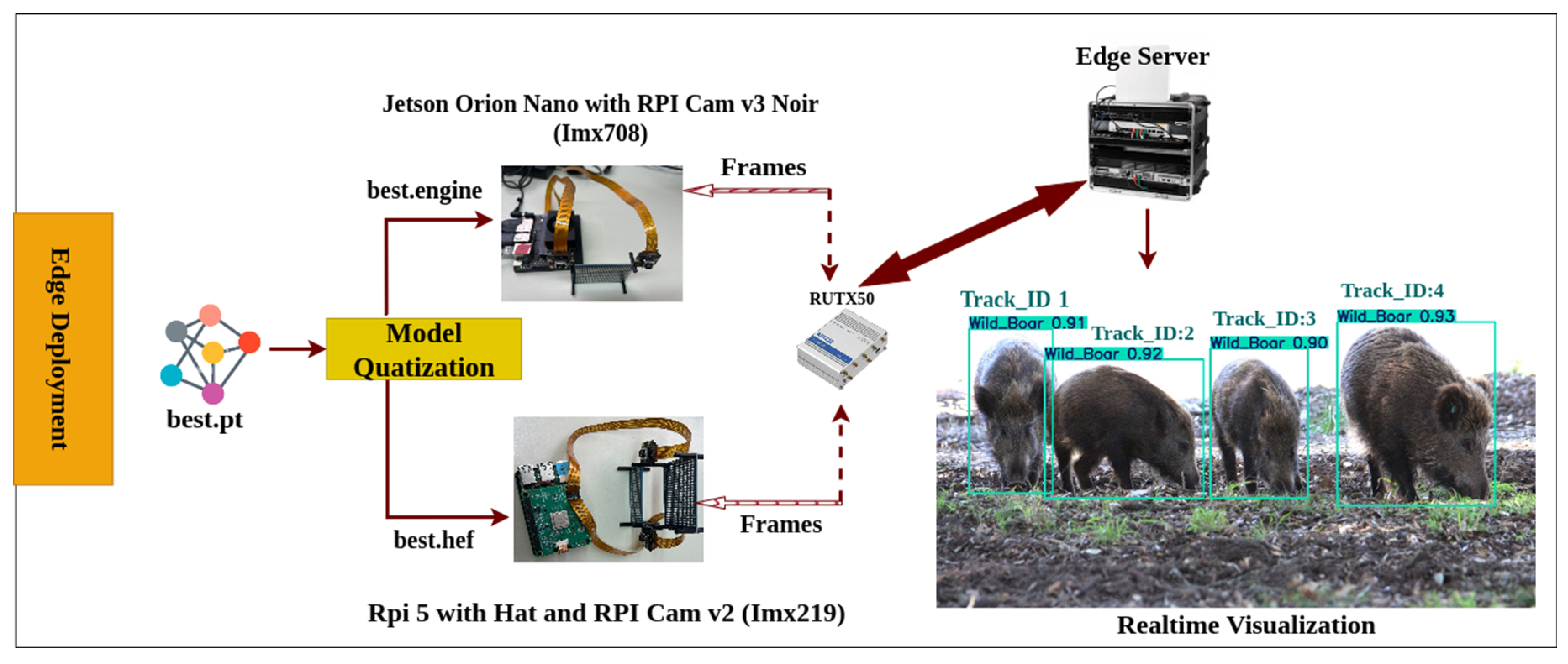
Our edge architecture has been strategically deployed in Parco di San Rossore, near our laboratory, in an area with abundant wildlife activity. To ensure seamless network connectivity across our edge setup, we placed a Teltonika RUTX50 router (accessed on 1 July 2025) approximately 600 m away from the edge server in Figure 1. The RUTX50 is a high-performance industrial grade 5G/4G LTE router featuring dual SIM slots for failover, Ethernet/Wi-Fi connectivity, VPN and firewall security, and remote management capabilities. It provides reliable and secure wireless connectivity in remote and outdoor environments. The edge server, a NOMAD 5G unit, is equipped with GPU/TPU acceleration, NVMe storage, and 5G, LTE, and Wi-Fi 6 connectivity. It handles real-time AI inference, data buffering, and CSV logging while supporting tools like Tailscale and Grafana for secure remote access and system monitoring. The edge deployment consists of two distinct configurations, one optimized for daytime wildlife monitoring and the other for nighttime operations. For night vision object detection, we utilize an NVIDIA Jetson Orin Nano Super Developer Kit (Orin Nano) (accessed on 1 July 2025), which delivers 67 TOPS of AI performance with 1024 CUDA cores and 32 Tensor Cores, based on NVIDIA’s Ampere architecture. The software stack includes CUDA (12.6.68), cuDNN (9.0.3), TensorRT (10.3.0), OpenCV (4.11.0), PyTorch (2.5.0a0+872d972e41.nv24.08), and Python (3.10.12), running on JetPack 6.2 with support for YOLOv8 (8.3.74), ONNX, and DeepStream (7.1). The board supports multiple I/O interfaces including MIPI CSI, GPIO, I2C, SPI, and PCIe. For imaging, we employ a CSI connected Raspberry Pi Camera Module 3 Wide-Angle NoIR (accessed on 1 July 2025), featuring the Sony IMX708 sensor. This sensor supports up to 12-megapixel resolution, CS- or M12-mount lens options for flexibility and is paired with a 48-LED (850 nm) IR crown (accessed on 1 July 2025) for effective night vision. This enables the capture of high-quality images even in total darkness, supporting accurate detection, tracking, and counting of animals at night. The daylight configuration features a Raspberry Pi 5 (Rpi5) (accessed on 1 July 2025) integrated with a Raspberry Pi Camera Module 2 (accessed on 1 July 2025) (Rpi CamV2), which features a Sony IMX219, 8-megapixel sensor an upgrade over the original 5-megapixel OmniVision OV5647 sensor. The RPi5 features a quad-core ARM Cortex-A76 CPU, PCIe 2.0, dual MIPI CSI, USB 3.0, and 40-pin GPIO, supporting lightweight AI inference with TensorFlow Lite (2.14.0), NCNN (v20250503), and OpenVINO (v2025.0), and is compatible with accelerators like the Hailo-8 and Coral TPU. Both sets of configurations continuously detect, track, and count objects, the presence of animals in the camera FOV, and transmit the processed frames to the edge server while also sending time-series data using MQTT publishers to Influxdb2 database. For enhanced monitoring, we use Grafana to visualize key performance metrics such as power consumption, bandwidth usage, and device health status remotely. For model deployment and optimization, we employed different inference techniques tailored to each edge device. On the Orin Nano, we remotely mounted the best.engine FP16 TensorRT model using a K3s Docker container (rancher/k3s:v1.33.2-k3s1), ensuring optimized inference speeds while balancing power consumption. The TensorRT-optimized model provides better frame rates (FPS) and lower latency compared to running a standard PyTorch model. In contrast, for Rpi 5 with Hailo-8 HAT, we deployed a quantized best.hef model, which takes advantage of the 13 TOPS computing power of the Hailo accelerator for efficient AI inference. The overall design of the system ensures a balance between accuracy, real-time performance, and energy efficiency, making it highly suitable for wildlife monitoring in remote areas.
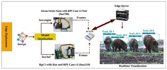
Figure 1.
Overview of the proposed edge-based wildlife monitoring framework integrating YOLOv8m detection with object tracking across resource constrained devices.
3.2. Dataset Collection and Annotations
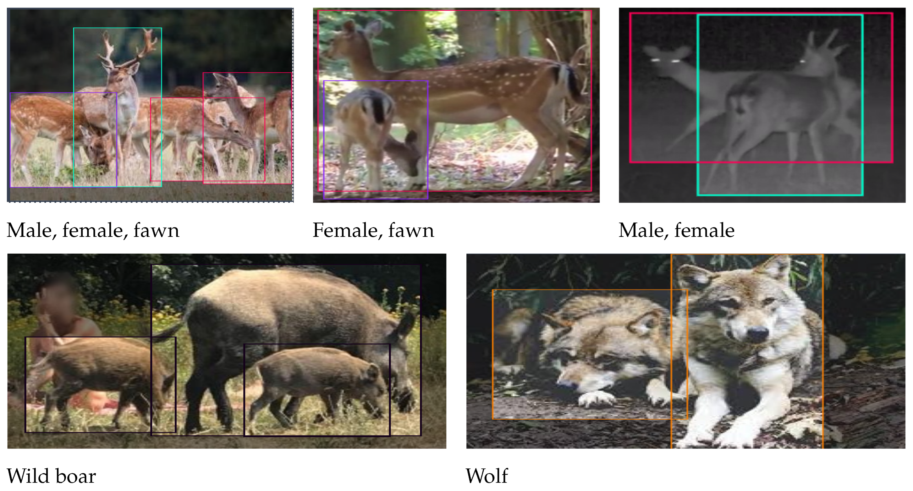
To train our YOLO model, the first and most essential step was to construct a high-quality dataset with accurate annotations. Our objective was to detect five specific animal classes commonly found in Parco di San Rossore: fallow deer (further divided into male, female, and fawn), wild boar, and wolf. Initially, we explored publicly available datasets from sources such as ImageNet, Google Open Images, Kaggle, Roboflow, and COCO. However, none of these datasets adequately represented the required combination of species and categories.
We also reached out to the park authorities to request access to relevant image and video data, but were unable to obtain it. As a result, we manually collected our dataset through short wildlife video clips triggered by motion sensors and camera trap images. During the assembling of the dataset, we carefully considered various environmental conditions, including day and night vision, high-resolution images, occlusions, and limited color visibility, to ensure robust model performance in real-world scenarios.
To construct the final dataset, we extracted frames from the videos and applied similarity checks to remove duplicates. Each class comprises approximately 2000 images, total 10,000 images across all five classes. Manual annotation was performed using the Roboflow Universe platform to maintain the high precision of the labeling shown in Figure 2. Finally, we split the dataset into training (70%), validation (20%), and testing (10%) subsets in Table 1, ensuring that each image was accompanied by a corresponding annotation file.

Figure 2.
Sample annotated images from the dataset.

Table 1.
Class distribution and train/validation/test split.
3.3. Neural Network Model Architecture
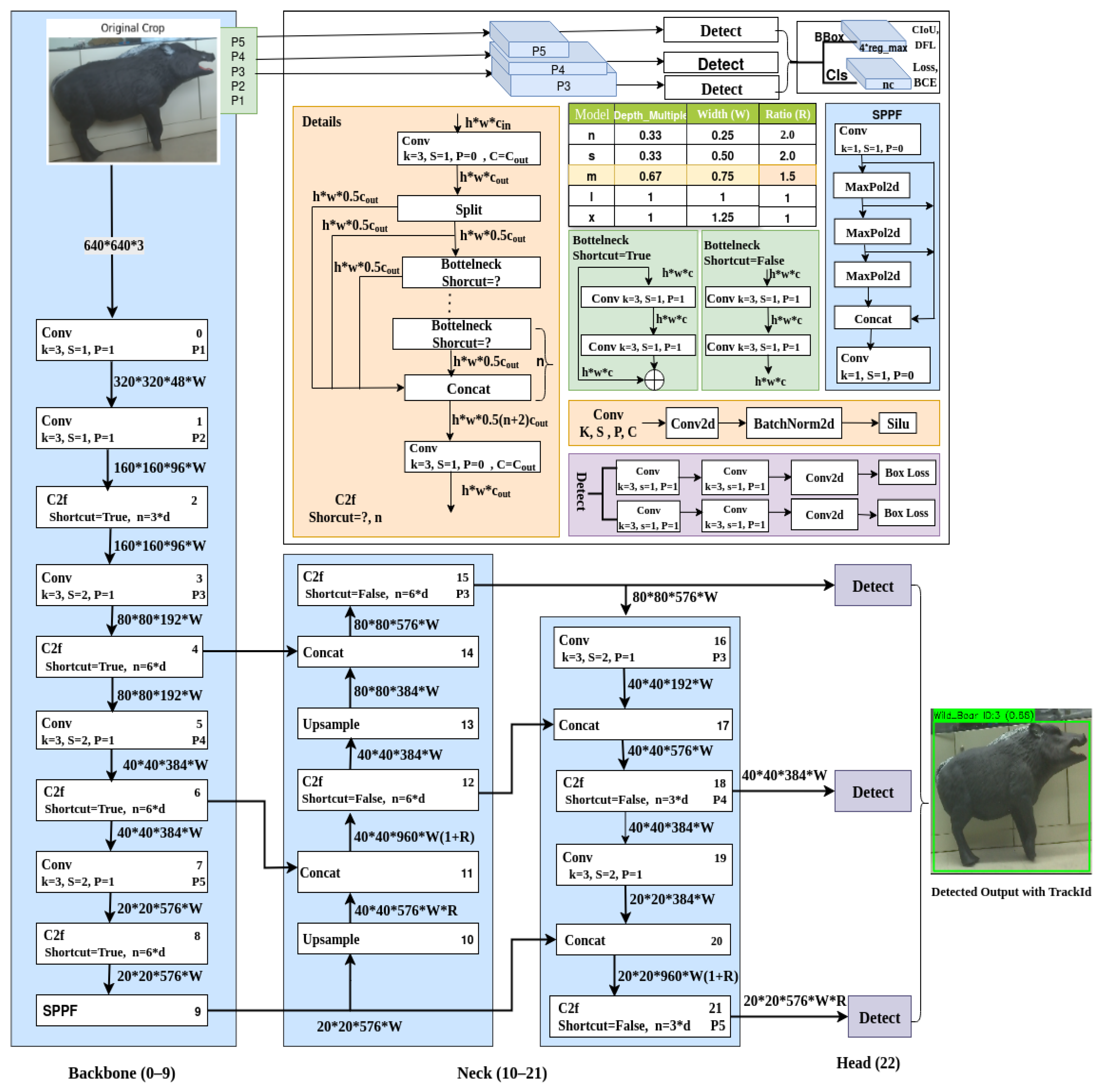
The YOLOv8m architecture is a highly optimized object detection framework designed to strike a balance between speed, accuracy, and computational efficiency. It consists of three main components: backbone, neck, and head. It uses three core building blocks: Convolutional Block (Conv), Cross-Stage Partial Fusion (C2F), and Spatial Pyramid Pooling Fast (SPPF). These components are scaled using the model scaling factors: depth 0.75, width 0.67, and ratio 1.25, allowing YOLOv8m to operate effectively on both high-performance and edge computing devices in Figure 3.
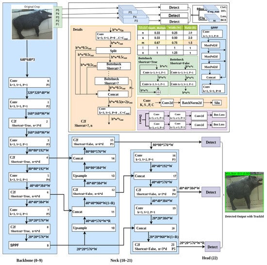
Figure 3.
Overview of the custom YOLOv8 architecture used in our wildlife detection framework.
3.3.1. Backbone
The Backbone is responsible for the initial feature extraction. It begins with a standard Conv block, consisting of a 2D convolution, batch normalization (BN), and a SiLU (Sigmoid-weighted Linear Unit) activation function. The convolution uses a 3 × 3 kernel, with the number of output channels determined by multiplying the base channel count by the width multiplier (e.g., 256 × 0.67 = 172). The SiLU activation is chosen over ReLU for its smooth gradient behavior, improving convergence and feature expressiveness.
Subsequent layers include multiple C2F (Cross-Stage Partial Fusion) blocks. The C2F block divides the input channels typically into 50% to pass through the identity and 50% to process via a stack of lightweight bottleneck blocks. The number of layers of bottleneck within C2F is calculated based on the depth multiplier (e.g., n = max(round(3 × 0.75), 1) = 2), where each bottleneck applies a residual path of 1 × 1 and 3 × 3 convolutions. The final output is a concatenation of all intermediate bottleneck outputs and the skipped input, enabling richer feature reuse and more stable gradient flow.
The final part of the backbone is the SPPF block, a speed-optimized variant of spatial pyramid pooling. Instead of parallel pooling with different kernel sizes, SPPF uses sequential 5 × 5 max pooling layers (three times), accumulating multiscale context without drastically increasing computational complexity. The outputs of the three pooling stages are concatenated along the channel axis with the original input and passed through a final 1 × 1 Conv layer to fuse the aggregated information. This design retains spatial information while maintaining runtime efficiency.
The backbone produces three key feature maps P3 (80 × 80), P4 (40 × 40), and P5 (20 × 20) at layers 4, 6, and 9, respectively, which carry low-level, mid-level, and high-level semantic features.
3.3.2. Neck
The Neck employs a hybrid FPN + PAN (Feature Pyramid Network + Path Aggregation Network) structure to fuse the multi-scale features from the backbone. Initially, deeper features (e.g., P5) are upsampled using nearest-neighbor interpolation, then concatenated with corresponding higher-resolution features (e.g., P4). This fused tensor passes through another C2F block, enhancing the refinement of the characteristics. The bottom-up PAN path further aggregates and propagates refined features down to higher resolution (P3), preserving spatial information critical for small object detection.
Each upsample fuse refine sequence uses 1 × 1 Conv layers to reduce channels, followed by concatenation and another C2F block to process the merged features. The combination of upsampling, skip connections, and multi-path fusion allows robust feature representation across scales while maintaining computational efficiency.
3.3.3. Head
The detection head is composed of lightweight Conv layers (primarily 1 × 1 and 3 × 3) that process each refined feature map independently (P3, P4, P5), and avoid complex residual or cross-stage connections to ensure fast inference. Each head produces predictions in the form of a tensor that encodes bounding boxes, objectness scores, and class probabilities, with the final output being P3 → 80 × 80 × 576, P4 → 40 × 40 × 384, P5 → 20 × 20 × 576. These outputs are optimized for the detection of large, medium, and small objects, respectively. The head uses anchor-free detection and applies non-maximum suppression (NMS) during inference to filter overlapping predictions. Finally, we obtain the detected objects as output with class names, confidence score, and bounding box.
3.4. Model Training Platform
The models were trained for up to 100 epochs, with an early stopping mechanism triggered at 75 epochs to prevent overfitting. Key hyper-parameters included a confidence threshold of 0.25, an initial learning rate of 0.01, and an adaptive batch size set to −1, allowing the system to automatically determine the maximum batch size supported by available memory. This configuration ensured optimal training speed and efficient utilization of hardware resources.
The training, validation, and testing phases were conducted on a high-performance platform featuring an Intel Xeon Cascade Lake processor running at 2.19 GHz with 8 cores, 24 GB of RAM, and an NVIDIA Tesla T4 GPU. The Tesla T4 offers 2560 CUDA cores, 320 Tensor Cores, 16 GB GDDR6 memory, a memory bandwidth of 320 GB/s, and a thermal design power (TDP) of 70 W.
The dataset was sourced from Roboflow [39], organized into train, validation, and test subsets, each accompanied by annotations and a data.yaml file specifying class names and file paths. After configuring the training parameters, the YOLOv8m model was trained on the Tesla T4 platform [40]. Upon completion, the training process generated a weights directory containing best.pt and last.pt model checkpoints, along with performance metrics, loss curves, and validation results. The best.pt model, which exhibited the highest accuracy, was selected for downstream tasks, including edge deployment. The final predictions demonstrate the robust capability of the model to accurately detect multiple classes of animals with high confidence scores.
3.5. Model Quantization for Deployments on Edge Devices
The model was trained with standard augmentation techniques, a learning rate scheduler, and early stopping based on mAP validation (mean average precision). After training, we achieved a final model with best.pt weights, yielding a mean average precision at intersection over union IoU 0.5 (mAP@0.5) of 92.3%, indicating high detection performance. To enable real-time inference on edge devices, we performed hardware-specific quantization and optimization. For Orin Nano, we converted best.pt into a TensorRT optimized engine file using the torch2trt and trtexec toolchain. INT8 quantization was applied using calibration data to improve inference speed while maintaining accuracy. The optimized model runs efficiently on the GPU, achieving higher FPS suitable for live object detection and tracking. For Rpi5 with Hailo-8L HAT, we converted best.pt to an intermediate ONNX format and then compiled it into a Hailo executable format (.hef) using the Hailo Model Zoo and HailoRT SDK. The quantization process was performed using the Hailo Post-Training Quantization (PTQ) pipeline, ensuring that the model met the memory and compute constraints of the Hailo-8 accelerator. By deploying the optimized models on these edge devices, we were able to achieve real-time wildlife detection and tracking performance in the field, enabling continuous monitoring.
4. Hybrid Algorithm for Tracking
In this section, we present the integrated tracking algorithm with the custom YOLOv8m object detection model, focusing on the real-time inference and visualization of detected and tracked frames in an edge computing environment. For motion tracking and object association across frames, we employed a Kalman filter-based approach, which effectively handles noisy detections and provides predictive tracking for moving objects. To address challenges such as occlusion and re-identification, we incorporated LBP matching for texture analysis, as well as HSV-based color histogram comparison. This hybrid strategy enables more robust identity preservation in cases where objects temporarily disappear or overlap in the FOV.
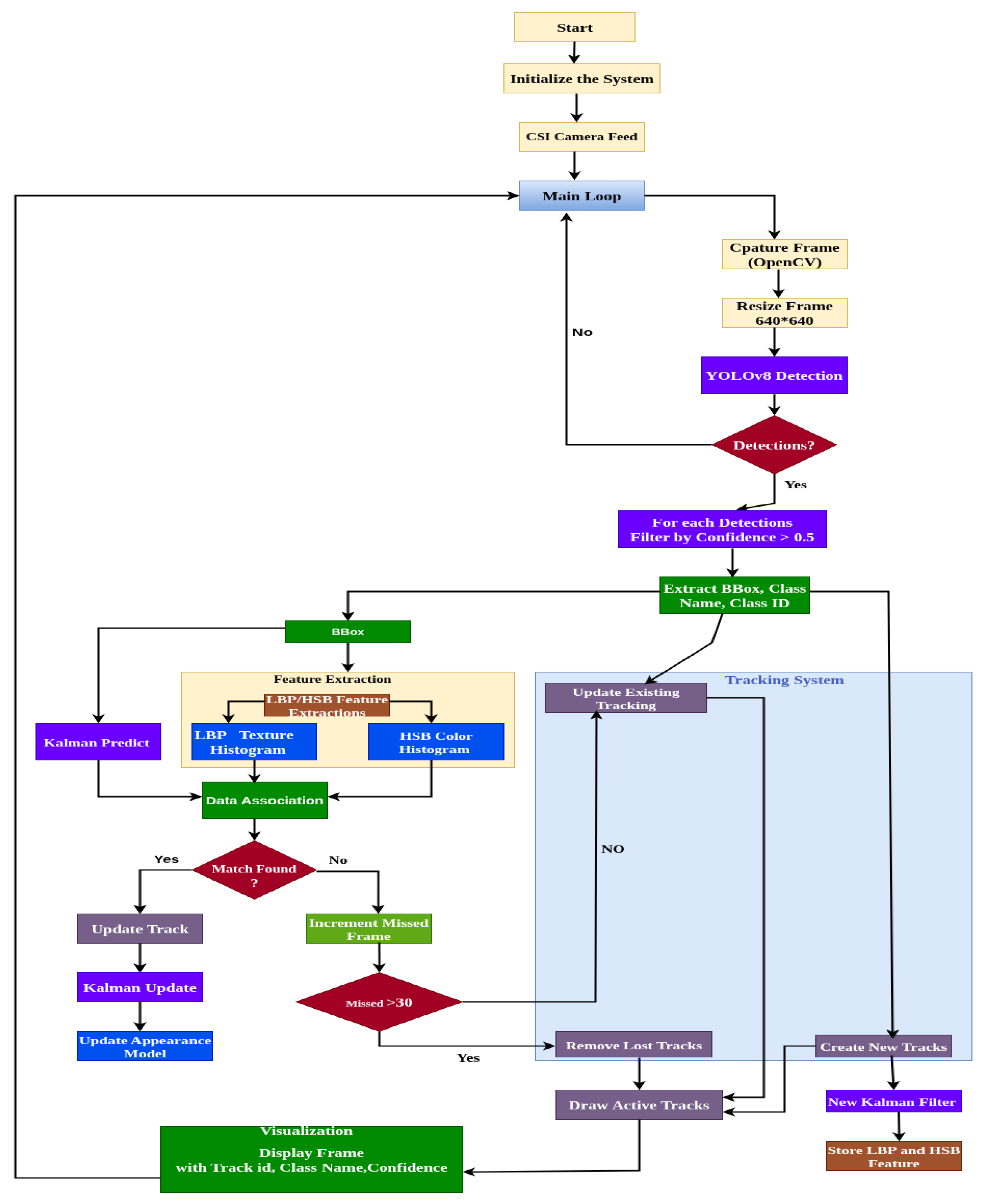
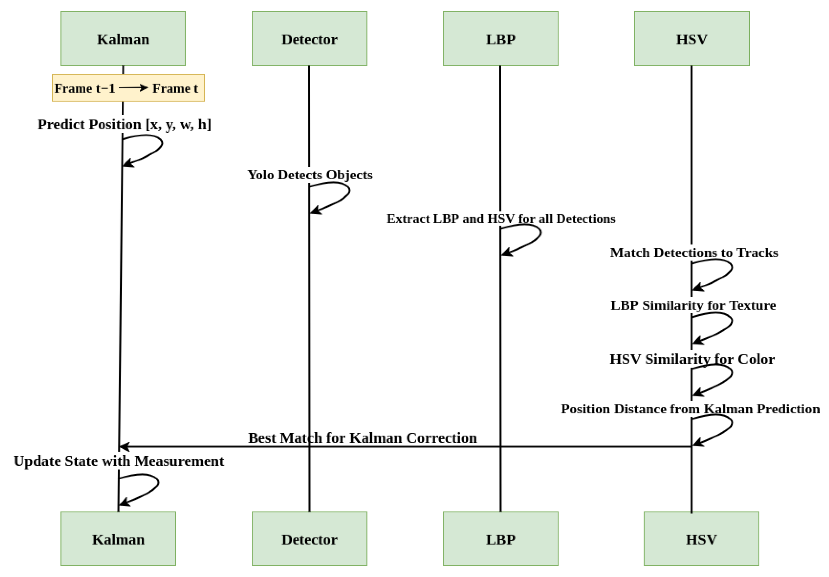
The tracking process operates in a step-by-step pipeline shown in Figure 4, optimized for edge continuum inference, with each module detection, prediction, feature matching, and re-identification designed for computational efficiency and reliability. In the following subsections, we detail each component of the tracking pipeline and its integration into the YOLOv8m-based detection framework.
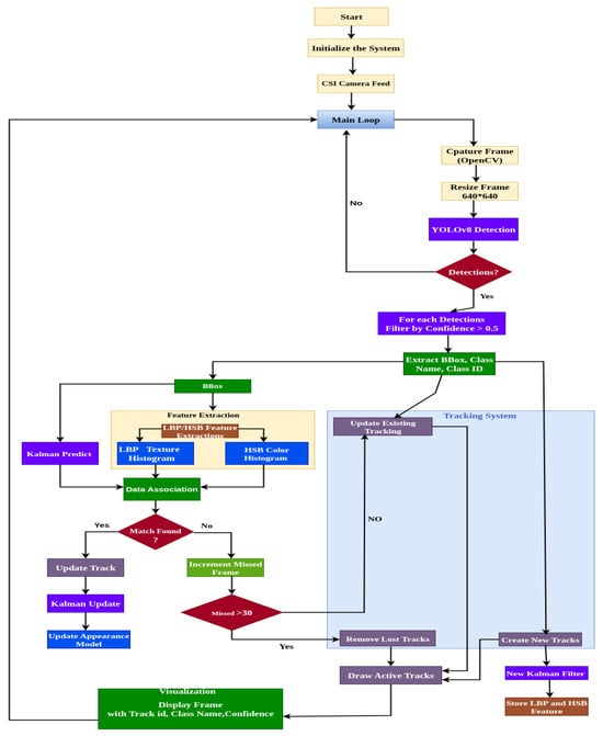
Figure 4.
Hybrid algorithm workflow for object detection and tracking.
4.1. CSI Camera Feed
When the system is initialized, the wildlife-monitoring system begins by connecting a CSI camera to an edge device, using a Rpi CamV3 (IMX708) with an Orin Nano or a Rpi CamV2 (IMX219) with an RPi5. Setting up the IMX708 camera with the Orin Nano was particularly challenging due to driver compatibility issues in JetPack 6.2. To solve this, we implemented a GStreamer pipeline inside an NVIDIA Ultralytics Docker container, since OpenCV alone could not directly access the CSI camera feed. We configured GStreamer to work with OpenCV by binding the pipeline, allowing us to capture frames and process them in real time. Once the camera feed was accessible, each frame was resized to 640 × 640 pixels, the default input size for the YOLOv8m model, before running inference. The model then provided bounding box coordinates, confidence scores, and class labels for the detected wildlife (discussed in Section 3). This approach ensures efficient real-time object detection while addressing hardware-specific challenges in edge deployments.
4.2. Object Detection with YOLOv8m Model
Our wildlife-monitoring system begins with YOLOv8 for real-time object detection. The model employs a CSPDarknet backbone to extract multiscale spatial features, while a PANet neck improves detection robustness across varying animal sizes. For each input frame at time t, YOLOv8 outputs a set of detections:
where represents the center coordinates of the bounding box, its width and height, the predicted class (e.g., deer, wolf), and the confidence score. To filter out false positives, detections with confidence scores below a predefined threshold are discarded.
To associate detections with existing tracks, we compute a cost matrix C where each element represents the dissimilarity between the i-th detection and the j-th predicted Kalman state . The cost is derived from the Intersection-over-Union (IoU) between the detection’s bounding box and the Kalman filter’s predicted bounding box (obtained by projecting the state via the measurement matrix H, which extracts positional coordinates). Specifically,
ensuring that lower values indicate better spatial overlap. The Hungarian algorithm then solves the assignment problem under two constraints:
- Class consistency: Detections and tracks must share the same animal class (e.g., a deer detection cannot match a wolf track)
- Minimum IoU threshold (): Rejects matches with insufficient overlap ()
This approach balances computational efficiency (critical for real-time tracking) with robustness to occlusions and false detections.
4.3. Tracking Algorithm Details
In our tracking framework, a hybrid method combining motion and appearance cues is employed to ensure robust and consistent object tracking. For each tracked object, the Kalman filter (KF) predicts its location in the current frame based on its previous state, allowing the tracker to handle temporary occlusions and maintain motion continuity. Simultaneously, we extract LBP histograms from the grayscale regions within each detected bounding box, providing compact and reliable appearance descriptors. Data association between detections and existing tracks is carried out using a two-step process. Initially, we compute the Intersection over Union (IoU) between predicted and detected bounding boxes and apply a gating threshold to eliminate unlikely matches. For the remaining candidates, we measure appearance similarity using the Pearson correlation coefficient () between their respective LBP histograms and , which quantifies the linear relationship between the two distributions. A weighted cost function combining both motion prediction and LBP-based appearance cues determines the final matching assignment. Once a detection is matched to a tracker, the KF state is updated with the new location, and the LBP descriptor is updated using an exponential moving average to maintain temporal consistency. If no match is found, the tracker continues relying on KF predictions until a predefined frame limit is reached. Additionally, to resolve ambiguities in cases where objects have similar textures but different colors, HSV histograms are incorporated as supplementary color features. This multi-cue strategy improves tracking performance in challenging scenarios involving occlusion, overlapping, or abrupt movement. The following sections explain every algorithm we used for our hybrid tracker design and how motion and appearance cues work together to enhance tracking accuracy.
4.4. Kalman Filter-Based Tracking
Our tracking system employs a constant velocity Kalman filter to maintain robust trajectories across occlusions and noisy detections in wildlife monitoring scenarios. The state vector represents each animal’s 2D position and velocity in pixel coordinates, where is the frame interval (e.g., 0.033 s for 30 FPS). The transition matrix propagates this state between frames assuming constant velocity, with , scaling the velocity contribution to position updates. During the prediction step (Equations (3) and (4)), the filter projects all tracks forward using the covariance, while the process noise grows to model unpredictable motion (e.g., sudden deer turns). For the updated step (Equations (5)–(7)), for object detection,
is associated with a track via IoU matching. The Kalman gain dynamically weights the correction term based on the detection confidence (encoded in ) versus the prediction uncertainty (from ). The state update (Equation (6)) adjusts positions more aggressively for high-confidence detections (low) but relies on predictions during occlusions. The measurement matrix extracts only positional observables as widths/heights are handled by the detector.
Prediction step:
Update step:
for matched pairs (detection and track ), the Kalman filter corrects its predicted state using the detection measurement :
where dynamically adjusted based on detection confidence . The track’s confidence score is updated exponentially:
For unmatched detections: New tracks are initialized with
For unmatched tracks: Tracks are retained for frames using pure predictions, and are terminated if their confidence drops below a threshold:
4.5. Local Binary Pattern (LBP) Transform
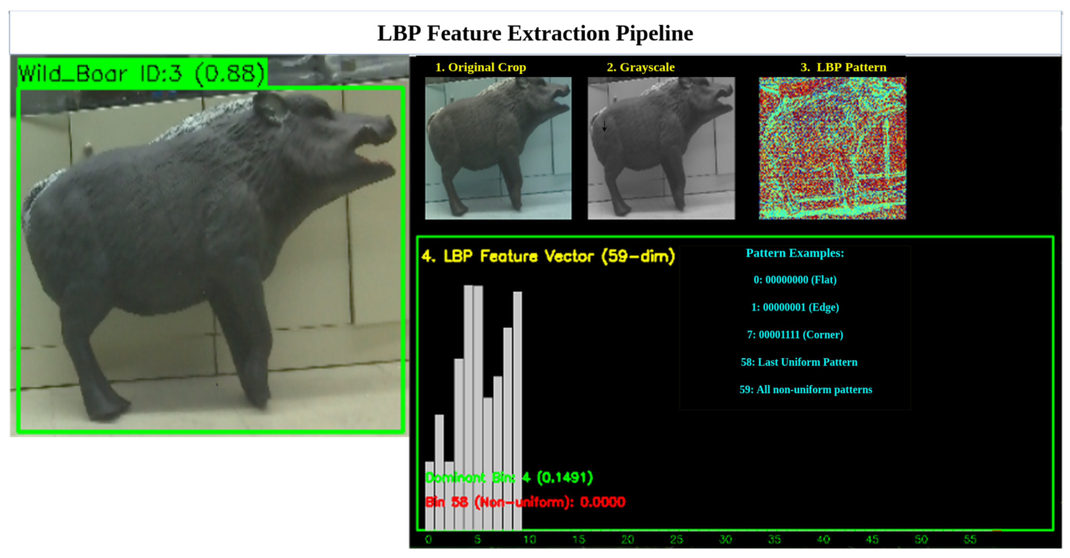
We apply the LBP transform to the grayscale image within each YOLOv8 detection bounding box to extract local texture features such as edges, flat regions, and corners. For each pixel, we compare it to its eight neighbors in a 3 × 3 grid and compute a decimal LBP code (0–255) that encodes local texture patterns. The resulting LBP and source images are saved for use in the next stage, supporting robust object re-identification and tracking. For each pixel in the grayscale image in Figure 5, excluding border pixels, consider its neighborhood .
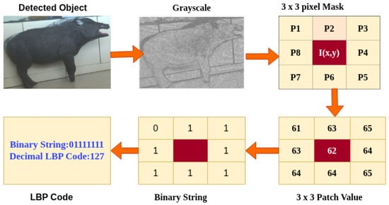
Figure 5.
A sample of extracting LBP calculation features.
Compare each of the eight neighboring pixels with the center pixel . For each comparison, assign a binary value:
The LBP code at position is then calculated as follows:
Here, denotes the intensity values of the eight surrounding pixels, ordered in a consistent clockwise or counterclockwise manner. This computation produces an 8-bit binary number in Figure 5, 01111111, which is converted into a decimal value in the range [0, 255] which is 127. The result is a matrix of LBP codes, where each pixel’s value represents a local texture descriptor. These descriptors are stored and used in the next stage for similarity matching across frames.
4.5.1. LBP Feature Representation (Histogram Construction)
This step is divided into three sub steps,
(I) Count LBP Codes: In this step, we initialize a 256-bin histogram H (one bin per possible LBP code).For each pixel , increment the histogram bin corresponding to its LBP value:
where is the indicator function (1 if true, 0 otherwise).
(II) Uniform Pattern Selection (Bin Reduction)
The selection of uniform patterns reduces the dimensionality of the LBP histogram by focusing on informative texture patterns. A binary LBP code is uniform if its circular representation has two or fewer transitions between 0 and 1 (e.g., 00000000, 00111100). With , there are 58 such patterns. All non-uniform patterns (with more than two transitions) are grouped into a single bin, reducing the histogram from 256 to 59 bins. This enhances computational efficiency and reduces noise. The uniformity measure U for an LBP code is
where is the binary value at position p, indicates a uniform pattern, indicates a non-uniform pattern.
(III) Normalization in Uniform LBP Histogram To make the LBP histogram comparable across different image regions or scales, normalization is applied by converting raw counts into probabilities. Each histogram bin , where , is normalized, and the sum of all normalized values of is 1, as follows:
The result is a 59-dimensional feature vector, ]. It represents the distribution of uniform and non-uniform texture patterns as probabilities in Figure 6, enabling robust texture analysis and classification.
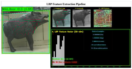
Figure 6.
Normalized 59-bin histogram representing uniform and non-uniform LBP patterns.
4.5.2. Feature-Based Tracking Using Histogram Similarity
For each detected object in the current frame, a normalized 59-bin histogram is computed and compared against a registry of existing object tracks from previous frames. The primary similarity metric is the Pearson correlation coefficient , which quantifies the linear relationship between two histograms and , as follows:
This correlation score ranges from (completely dissimilar) to 1 (perfectly similar), and is efficiently computed using OpenCV’s cv2.compareHist(⋯, cv2.HISTCMP_CORREL) function. The similarity value of LBPsim is added in the data association for the matching steps.
4.6. HSV-Based Tracking
The HSV algorithm is integrated to handle similar-looking objects for robust tracking with the LBP and Kalman filter algorithm. The algorithm comprises the following steps.
4.6.1. BGR to HSV Conversion
To enhance the tracker’s appearance matching, the color information of detected animals is encoded in the HSV color space, which is more perceptually uniform than RGB. The conversion from RGB to HSV follows normalization:
The value channel is defined as follows:
The saturation is computed as follows:
The Hue calculation depends on which RGB channel holds the maximum value:
Finally, OpenCV scales the hue to the range :
This transformation enables a more robust color-based comparison in varying lighting conditions when computing HSV histograms for track appearance similarity.
4.6.2. Color Masking
Color masking is used to isolate pixels in an image that falls within a specified HSV color range. Each pixel p in the image is represented as follows:
We define lower and upper threshold values for each component:
The binary mask function is defined as follows:
This operation produces a binary mask where the selected pixels (value 1) correspond to a desired color region. It is used to calculate more robust HSV histograms in the tracker appearance model.
4.6.3. 2D Histogram Calculation
To find the appearance of tracked animals, we computed a 2D joint histogram over the Hue and Saturation (HS) components in the HSV color space. For each pixel where the color mask is valid (), we assign the corresponding hue and saturation values to the histogram bins. The joint histogram accumulates the count of pixels whose hue falls in the bin i and saturation in the bin j, defined as follows:
Each bin spans the interval , where , and similarly for saturation. To ensure that the histogram is invariant to region size, we normalize it as follows:
where is a small constant added to prevent division by zero. This normalized histogram is used to compare appearance features between detected and tracked objects using similarity measures. Figure 7, illustrates the transformation of the color space for the fallow class of male deer, where the original BGR image is converted to the HSV color space. From this transformation, we compute separate histograms for the hue and saturation channels, visualized as red and green distributions, respectively. This representation effectively captures the distinct chromatic characteristics of the subject, with hue values (red) indicating color dominance and saturation values (green) reflecting color intensity. The dual-channel histogram provides a comprehensive analysis of the animal’s coloration patterns under varying lighting conditions.
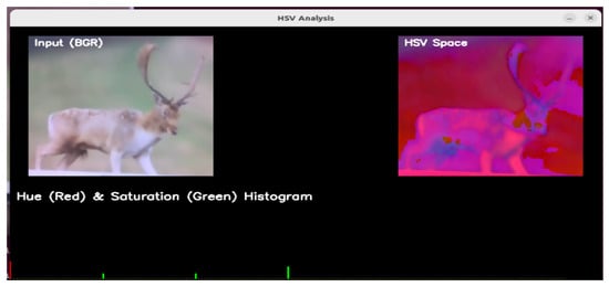
Figure 7.
Hue and saturation 2D joint histogram.
4.6.4. Histogram Comparison for Re-Identification
To compare the appearance of tracked objects across frames, use histogram-based similarity metrics. Specifically, we computed the correlation coefficient between two normalized 2D histograms P and Q, which represent the color distributions of two object regions in the HSV space. The correlation coefficient is defined as follows:
where and are the mean values of the histograms, and are the values of the bin i in the normalized histograms P and Q, respectively, and N is the total number of bins. This correlation score ranges from (completely dissimilar) to 1 (identical) and provides a robust measure for comparing the appearance of objects by taking into account both the shape and distribution of color intensities in the HSV space. It is particularly effective in Re-ID tasks where lighting or slight orientation changes may occur between frames.
4.7. Data Association for Matching
In the entire algorithm pipeline, our data is associated as shown in Figure 8. All algorithms, such as the Kalman filter, the LBP, and the HSV histogram, are combined using a weighted sum.
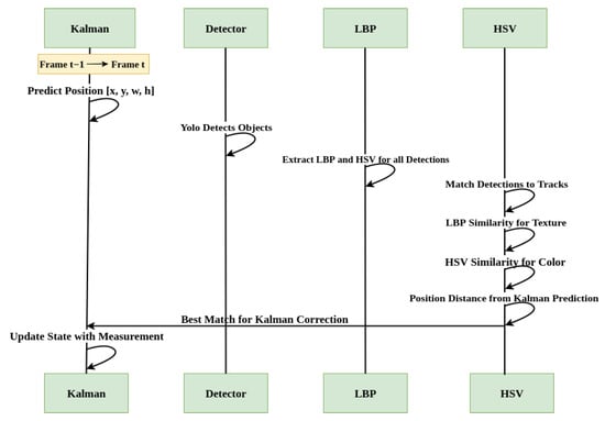
Figure 8.
Data association and update of the tracking parameters.
In this phase, tracked objects are associated with new detections using a matching score computed as a weighted sum of multiple similarity metrics. The total score is defined as follows:
where and are histogram correlation scores computed using LBP and HSV features, respectively (e.g., via OpenCV’s HISTCMP_CORREL function). The position similarity is calculated as follows:
which normalizes the Euclidean distance between the predicted Kalman position and the detected position z on a spatial scale of 100. The size similarity compares bounding box areas. In our implementation, the weights used are: , , , and , reflecting the relative importance of each feature in the association process.
4.8. Tracking and Counting
This step forms the backbone of the entire detection and tracking pipeline, integrating Kalman filter-based motion prediction with appearance-driven data association to maintain consistent object identities across frames. Initially, detections are sorted by confidence to prioritize reliable matches. Each active track predicts its next position, and unmatched detections are compared using a composite similarity score that combines LBP texture, HSV color histograms, spatial proximity, and bounding-box size similarity. A match is confirmed if the score exceeds a defined threshold , allowing the track to be updated while preserving temporal identity and avoiding duplicate counts for the same object. If no match is found, the track persists for a limited number of frames (max occlusion) to support occlusion handling. New unmatched detections initialize fresh tracks with unique IDs and extracted features. For each new track, a per-class counter is incremented, ensuring accurate, non-redundant object counts (e.g., deer, wild boar) while maintaining tracking stability. This mechanism achieves a balance between counting precision, occlusion robustness, and identity preservation in dynamic, multi-object environments.
4.9. Saving the Frame and Time-Series Data to Send Edge Server
In this step, we log time-series data in a CSV file for every detection, including the frame number, track ID, bounding box coordinates (x, y, width, height) and object class, confidence score, visibility flag, where 1 indicates full visibility and 0 denotes occlusion according to the format of multi-object tracking benchmark (MOT1.1) [41]. When a new track_ID is assigned or a new animal class is detected, the corresponding frame is saved inside the container for later use in behavioral analysis and population estimation. Moreover, we publish structured JSON messages through the Paho MQTT client to a local broker, which are subscribed to and processed by Telegraf. Telegraf parses and forwards these data to InfluxDB v2, enabling high-performance time-series storage and querying. This pipeline ensures low-latency data transfer to the edge server, where it can be visualized or analyzed for trends, habitat activity, and conservation metrics in the Grafana dashboard in Figure 9.
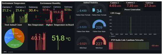
Figure 9.
Animal distribution Grafana dashboard.
5. Experimental Evaluation Metrics
To assess the effectiveness of this approach, we evaluate the tracking pipeline using standard multi-object tracking metrics that measure overall tracking quality, identity consistency, and the balance between detection and association. These metrics are Multiple Object Tracking Accuracy (MOTA) [42], Higher-Order Tracking Accuracy (HOTA) [43], and Identity F1 Score (IDF1) [44], each offering complementary insights into tracking performance.
5.1. Multiple Object Tracking Accuracy (MOTA)
MOTA is a comprehensive metric that simultaneously penalizes false negatives (FNs), which means the number of missed detections, false positives (FPs), defined as not matched to any ground truth, and identity switches (IDSW), defined as the number of times the identity of a 535 tracked object changes incorrectly, providing a scalar value that summarizes overall tracking quality. Mathematically, MOTA is expressed as follows:
where GT represents the total number of ground-truth objects across all frames. A higher MOTA value (closer to 1) indicates fewer tracking errors, while a negative MOTA suggests that tracking errors exceed correct detections. In the context of wildlife monitoring, MOTA serves as a critical indicator of the overall reliability of the tracker when detecting and consistently maintaining object tracks across frames under resource-constrained edge conditions.
5.2. Higher-Order Tracking Accuracy (HOTA)
While MOTA offers a global summary of errors, HOTA provides a more balanced and detailed evaluation by decoupling tracking performance into detection and association accuracy. It is defined as the geometric mean of the detection accuracy (DetA) and association accuracy (AssA), calculated as follows:
Here, detection accuracy is given by the following:
and the association accuracy is calculated as follows:
where TP represents true positive detections, and measures correctly associated detections over time. HOTA ranges from 0 to 1, with higher values indicating better tracking performance in both detection and association. For our use case, HOTA reveals how well the tracker balances accurate detection with consistent identity assignment, essential for real-time tracking of animals under challenging and dynamic environmental conditions.
5.3. Identity F1 Score (IDF1)
To assess the tracker’s ability to preserve identity between frames, we employ the IDF1, which measures the consistency of the assignment of identification throughout the sequence. The IDF1 score is defined by the following:
Here, IDTP denotes the number of correctly identified detections over time, IDFP represents incorrect identity assignments, and IDFN corresponds to ground truth identities that were missed. This metric is computed to find the optimal one-to-one mapping between predicted and ground-truth identities. Ranging between 0 and 1, IDF1 provides a direct measure of the tracker’s ability to maintain identity integrity across frames. In smart wildlife monitoring, a high IDF1 score is crucial for behavioral analysis and ecological studies, as misidentifying animals or fragmenting their trajectories could lead to incorrect insights about movement patterns or group behavior.
6. Result Analysis
On edge platforms, our software supports real-time detection and tracking and logs the prediction results into a CSV file following the MOT1.1 format. The system also records videos of when animal movement is detected within the camera’s FOV. In addition, it counts and stores frames when an animal is actively tracked, a tracking ID is switched, or a new animal (of a different class) enters the frame.
The overall accuracy of these services heavily depends on the performance of the tracker. To evaluate our hybrid tracker, we compare its performance with BoTSORT and Byte Track on the same video. For this purpose, we use the recorded video along with ground-truth annotations created using CVAT. Our hybrid tracker generates outputs in the standardized MOT Challenge 1.1 format, as illustrated in Table 2, which shows a representative sample of the results of the night event of wild boars tracking. This format requires each detected object to be represented as a single line containing ten comma-separated values, with the final three fields (representing 3D world coordinates) set to −1 for 2D tracking scenarios. Furthermore, we analyze the impact of the tracker on system efficiency by measuring how many frames or time-series data packets must be sent to the edge server and the corresponding power and bandwidth usage per frame. This allows us to calculate the percentage savings in power and bandwidth achieved by using the tracker and compare it to a baseline system without tracking.
Table 2.
Object tracking data MOT1.1 format.
Table 3 represents a comparative analysis of three tracking methods: Hybrid, BoT SORT, and Byte Track across different event scenarios involving animal tracking under varying lighting conditions, such as wild boar at night and wolves during both day and night. For each event, key metrics are reported to assess tracking performance. These include the number of frames in the video, ground-truth objects, and predicted objects, as well as the number of ground-truth and predicted identities. Each tracker is evaluated using standard multi-object tracking metrics: MOTA, HOTA, and IDF1, along with supporting figures such as FNs, FPs, IDSW, and identity-based statistics like IDTP, IDFP, and IDFN.
Table 3.
Comprehensive comparison of tracking performance metrics (MOTA, HOTA, IDF1) across different trackers (Hybrid, BoT-SORT, ByteTrack) under varying environmental conditions (day/night vision) and scenarios (wild boar, wolf tracking). The table includes detection and association metrics along with frame and object statistics.
In the Wild Boar Night Vision scenario, the video consists of 192 frames and involves tracking two ground-truth identities over 384 objects. The hybrid tracker slightly outperforms BoT SORT and Byte Track in terms of IDF1, achieving a score of 0.71, suggesting better identity consistency. MOTA is also the highest for hybrid at 0.597, while BoT SORT and Byte Track both achieve around 0.585. Although all trackers encounter some false negatives and positives, the Hybrid maintains a lower ID switch count and more stable ID tracking performance. For Wolf Day Vision, the tracking task appears to be straightforward. All three trackers achieve perfect scores on all metrics, MOTA, HOTA, and IDF1 are each 1.0, with zero false detections or ID switches. This indicates highly ideal conditions in the video, such as consistent lighting and clear object motion, which allowed all trackers to perform flawlessly.
In contrast, the Wolf Night Vision scenario includes 798 frames and presents more challenging conditions due to poor lighting. Even so, all three trackers still perform well, achieving an IDF1 score of 0.95 and zero ID switches, suggesting strong identity preservation even in difficult visibility. MOTA values are slightly reduced to 0.90, and false negatives are higher, with 76 missed detections, likely caused by the lower image clarity in night vision. The overall consistency in tracker performance for this scenario demonstrates robustness in identity tracking, even though a few detections were missed.
Figure 10 illustrates the radar view of object tracking performance, which confirms hybrid balanced performance across MOTA, HOTA, IDF1, DetA, and AssA, with a notably larger coverage area in difficult conditions. In contrast, BotSort/ByteTrack excel only in simpler scenarios (e.g., Wolf Day/Night), where all trackers achieve perfect scores (MOTA = 100%, IDF1 = 100%, AssA = 100%) due to ideal detection conditions.
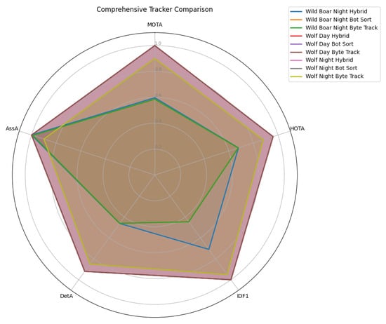
Figure 10.
Radar view of object tracking performance over time.
6.1. Trajectory Analysis
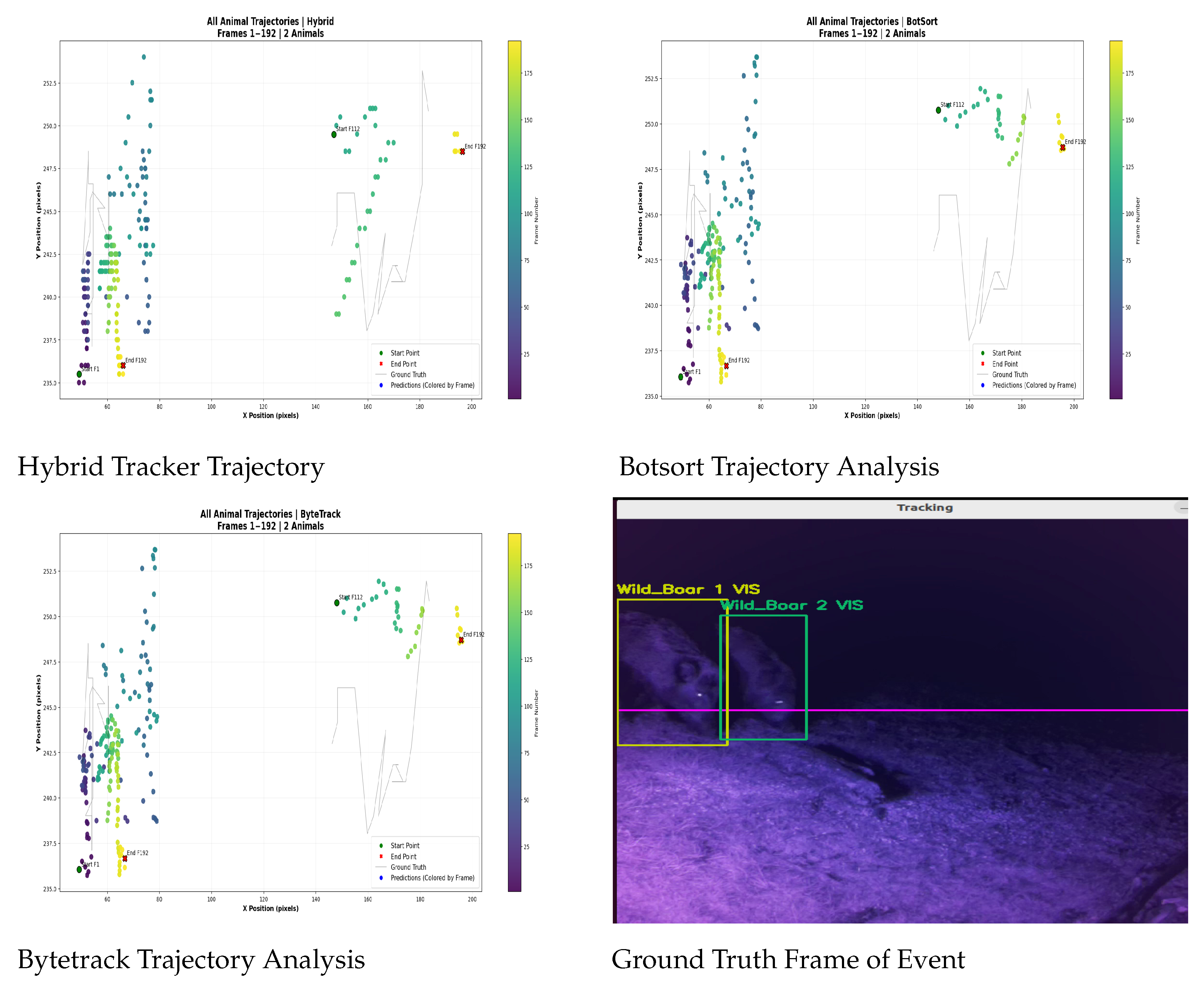
The tracking performance during the Wild Boar Night event (two animals) demonstrates nearly identical effectiveness across all three algorithms, with subtle advantages for the hybrid tracker in Table 4. All methods maintained excellent identity preservation (just 1 ID switch across each 192 frames) and comparable coverage (59.6% of frames). While BotSort and ByteTrack showed identical metrics (0.777 IoU, 8.36 px error), the hybrid tracker achieved marginally superior precision with a 0.778 IoU and reduced position error (8.00 px), suggesting better handling of the animals’ nighttime movements through vegetation. The consistent single ID switch indicates all trackers successfully maintained distinct identities for both boars despite challenging low-light conditions, though the hybrid method’s slightly lower positional error implies more accurate path reconstruction when animals crossed or moved through obscured areas. This performance parity suggests robust baseline tracking capabilities, with the hybrid method showing potential advantages in positional accuracy during complex nocturnal movements. Figure 11 illustrates the tracking of two wild boars across video frames. The ground truth indicates both animals (ID1 and ID2) with visibility flags. The tracker successfully follows ID1 continuously from frame 1 to 192, while ID2 is tracked from frames 111–149 and again from 179–192. The left side of each tracker plot shows ID1’s movement, and the right side shows ID2’s. This visual representation helps in easily analyzing the animals’ trajectories, which is crucial for studying their behavior.
Table 4.
Tracking performance comparison for the Wild Boar Night event.

Figure 11.
Trajectory analysis of all trackers of the night event.
6.2. Occlusion Handling
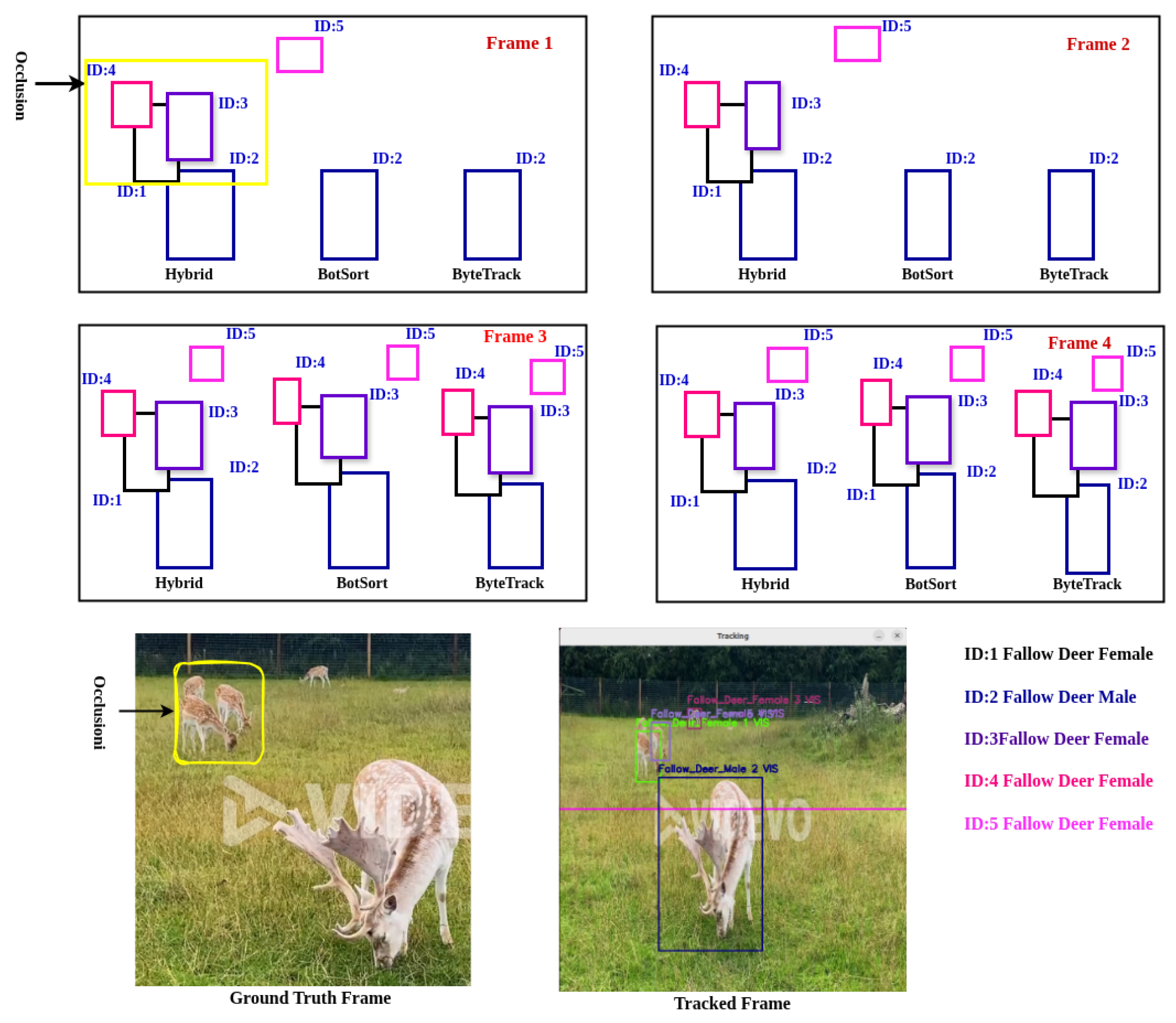
To evaluate occlusion handling, we selected a daytime event involving fallow deer, where five animals are present in the ground truth frame in Figure 12. In the first four frames, three animals become partially or fully obscured by others, indicated by the yellow box labeled as occlusion. Beyond the fourth frame, the sequence contains no further occlusions.
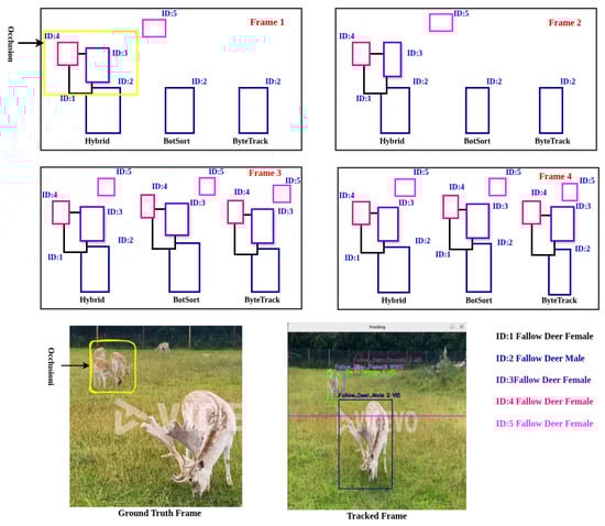
Figure 12.
Occlusion handling scenario of all trackers.
Our comparative analysis with GT annotations demonstrates that the proposed hybrid tracker outperforms both BoT-SORT and ByteTrack in occlusion handling. As shown in Figure 12, in the case of frame 1 and frame 2, the hybrid tracker successfully handles occlusions beginning from the first frame by detecting all the animals inside the occlusion yellow box, while the other two trackers only begin to manage occlusions starting from frame 3. Both BoT-SORT and ByteTrack fail to maintain consistent object identities during the occlusion period, whereas the hybrid tracker accurately tracks all animals despite visual overlaps.
6.3. Power Estimation for Detection and Tracking Services
Table 5 highlights the performance and power consumption differences between detection-only and detection-with-tracking services across various platforms and lighting conditions for sending time-series data to the edge server. Sending one frame from the edge device consumes 0.01 watts/s. In detection-only systems, power consumption is calculated as follows: 0.01 × number of detected animals per frame × total frames. For example, in the Fallow Deer day vision case with 522 frames and five animals per frame, detection only consumes 26.1 W, while the tracking-based service sends only one frame per unique ID (5 frames), using just 0.05 W, a negligible amount. Moreover, detection-only services count animals per frame, leading to inflated counts (e.g., 384, 1004, 798, 2610), while tracking maintains identity over time, yielding accurate counts (2, 2, 1, 5, respectively). Power Saving (%):
Table 5.
Event detection and tracking summary with power savings.
Power Reduction Factor:
Across all tested events and platforms, object tracking reduced power consumption by over 99.4%, achieving power reduction factors ranging from 192× to 798×, directly proportional to the number of redundant detected object time-series data suppressed during tracking. This highlights that power savings scale linearly with frame count reduction, enabling ultra-efficient edge deployment. These results also confirm that integrating the tracking drastically reduces energy consumption and significantly improves counting accuracy and consistency over time.
6.4. Bandwidth Estimation in Detection-Only and Tracking Scenario
Frames are captured from a CSI camera using a GStreamer pipeline configured with a capture resolution of pixels at 30 frames per second. The pipeline utilizes the nvvidconv plugin to perform hardware-accelerated downscaling to pixels, reducing data volume while preserving essential spatial information. Subsequently, each frame is resized to using OpenCV’s cv2.resize() to match the input resolution expected by the object detection model. At 30 frames per second, the data generated without tracking is as follows:
Over a 10 s window, this results in the following:
To reduce this load, we implemented object tracking, which ensures only the first frame of a consistently tracked object is transmitted. Therefore, only one encoded frame (717 KB) is sent in 10 s:
The bandwidth saving from using tracking is as follows:
Reduction factor:
This 300× bandwidth reduction is achieved without compromising detection accuracy, enabling scalable and power-efficient wildlife monitoring. Figure 13 compares the bandwidth usage of two edge AI pipeline configurations detection only and tracking against practical Wi-Fi capacities (Wi-Fi 4, 5, and 6). The detection-only pipeline consumes approximately 172 Mbps, which significantly exceeds the bandwidth typically supported by Wi-Fi 4 and 5 in resource-constrained environments. In contrast, the tracking configuration uses just 0.57 Mbps, demonstrating its suitability for low-bandwidth, real-time deployment over wireless networks.
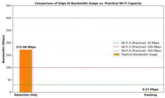
Figure 13.
Bandwidth comparison of edge AI with WiFi capacity.
7. Conclusions and Future Work
We present a highly efficient, identity-preserving animal monitoring pipeline designed for edge deployment in real-world wildlife observation scenarios. By combining robust object detection with hybrid tracking, our system demonstrated consistent performance across varied conditions, including daytime and nighttime recordings, and under challenging occlusions such as vegetation or low visibility.
Evaluation against leading trackers, including BoT-SORT and ByteTrack, showed that our method achieves superior positional accuracy, reduced ID switches, and high identity preservation, even in sequences with multiple animals. In addition to strong tracking accuracy, our pipeline introduces a significant advancement in energy and bandwidth efficiency. Unlike detection-only approaches that transmit redundant frames and inflate animal counts, our system sends only those detected animal frames if a new track_id is assigned, or an id switch, or a new animal comes with existing animals in the FOV, but not every frame for the same animals detected in a number of consecutive frames. This results in up to 99.87% bandwidth savings and over 99.67% power reduction, enabling sustained operation on low-power, network-limited edge devices. The power reduction scales linearly with the decrease in transmitted frames, ensuring optimal resource usage without compromising detection quality. Moreover, by maintaining consistent object identities, our tracking-based approach ensures accurate animal counting over time, correcting the inflated numbers common in detection-only systems. These characteristics make the pipeline especially suitable for deployment in remote, power-constrained environments where reliability, minimal transmission, and accurate behavioral analysis are critical. Together, these results confirm that integrating intelligent tracking not only enhances accuracy but also enables scalable, cost-effective, and environmentally sustainable wildlife monitoring using edge AI technologies.
Looking forward, planned enhancements, including Extended Kalman filters for nonlinear motion modeling, adaptive confidence thresholding, lightweight deep ReID modules, and multi-modal sensor fusion, will further elevate the system’s robustness in crowded or visually ambiguous environments. In addition, integrating trajectory analysis will enable the extraction of movement patterns and behavioral insights from tracked animals over time, such as activity zones, interaction events, and migratory behaviors. The adoption of federated learning frameworks and expansion to multi-camera ecological networks will enable collaborative, privacy-respecting monitoring across larger areas and longer timescales. Ultimately, this work lays a solid foundation for scalable, intelligent, and energy-aware wildlife-monitoring systems that can support real-time biodiversity research, conservation efforts, and automated ecological insight generation across diverse habitats.
Author Contributions
Conceptualization, M.A.R., S.G. and M.P.; methodology, M.A.R., S.G. and M.P.; software, M.A.R.; validation, M.A.R., S.G. and M.P.; formal analysis, M.A.R., S.G. and M.P.; investigation, M.A.R., S.G. and M.P.; resources, M.A.R., S.G. and M.P.; data curation, M.A.R. and S.G.; writing—original draft preparation, M.A.R. and S.G.; writing—review and editing, M.A.R., S.G. and M.P.; visualization, M.A.R., S.G. and M.P. All authors have read and agreed to the published version of the manuscript.
Funding
This work was partially supported by the Italian Ministry of Research (MUR) in the framework of the FoReLab project (Departments of Excellence) and by the European Union—Next Generation EU under the Italian National Recovery and Resilience Plan (NRRP), Mission 4, Component 2, Investment 1.3, CUPE83C22004640001, partnership on “Telecommunications of the Future” (PE00000001-program “RESTART”).
Data Availability Statement
The data presented in this study are available on request from the first author. The data are not publicly available due to privacy restrictions.
Acknowledgments
We acknowledge the use of ChatGPT (https://chat.openai.com/, accessed on 1 July 2025) for English correction and rephrasing in some sections of the manuscript. It was not used to generate new content or ideas; it was employed only as a tool to enhance the smoothness and correctness of the existing text.
Conflicts of Interest
The authors declare no conflicts of interest.
Abbreviations
Acronyms and abbreviations used in this paper:
| AI | Artificial Intelligence |
| AssA | Association Accuracy |
| BN | Batch Normalization |
| BGR | Blue Green Red |
| Conv | Convolution |
| C2F | Cross Stage Partial Fusion |
| DetA | Detection Accuracy |
| FN | False Negative |
| FP | False Positive |
| FOV | Field of View |
| FPN | Feature Pyramid Network |
| FPS | Frame per Second |
| GT | Ground Truth |
| HSV | Hue Saturation and Value |
| HOTA | Higher-Order Tracking Accuracy |
| IDF1 | Identity F1 Score |
| IoU | Intersection Over Union |
| IDSW | ID Switch |
| LBP | Local Binary Pattern |
| MOT | Multi-Object Tracking |
| MOTA | Multiple Object Tracking Accuracy |
References
- Cervi, A.L.; Poling, K.R.; Higgs, D.M. Behavioral measure of frequency detection and discrimination in the zebrafish, Danio rerio. Zebrafish 2012, 9, 1–7. [Google Scholar] [CrossRef] [PubMed]
- Ferrante, G.S.; Vasconcelos Nakamura, L.H.; Sampaio, S.; Filho, G.P.R.; Meneguette, R.I. Evaluating YOLO architectures for detecting road killed endangered Brazilian animals. Sci. Rep. 2024, 14, 1353. [Google Scholar] [CrossRef] [PubMed]
- Zwerts, J.A.; Stephenson, P.J.; Maisels, F.; Rowcliffe, M.; Astaras, C.; Jansen, P.A.; van der Waarde, J.; Sterck, L.E.H.M.; Verweij, P.A.; Bruce, T.; et al. Methods for wildlife monitoring in tropical forests: Comparing human observations, camera traps, and passive acoustic sensors. Conserv. Sci. Pract. 2021, 3, e568. [Google Scholar] [CrossRef]
- Redmon, J.; Farhadi, A. YOLO9000: Better, Faster, Stronger. In Proceedings of the 2017 IEEE Conference on Computer Vision and Pattern Recognition (CVPR), Honolulu, HI, USA, 21–26 July 2017; pp. 6517–6525. [Google Scholar] [CrossRef]
- Sapkota, R.; Qureshi, R.; Flores-Calero, M.; Badgujar, C.; Nepal, U.; Poulose, A.; Zeno, P.; Bhanu Prakash Vaddevolu, U.; Yan, H.; Karkee, M. YOLO11 to Its Genesis: A Decadal and Comprehensive Review of The You Only Look Once (YOLO) Series. Springer. 2024. Available online: https://ssrn.com/abstract=4874098 (accessed on 27 October 2024).
- Vijayakumar, A.; Vairavasundaram, S. YOLO-based Object Detection Models: A Review and its Applications. Multimed. Tools Appl. 2024, 83, 83535–83574. [Google Scholar] [CrossRef]
- Wang, X.; Li, H.; Yue, X.; Meng, L. A Comprehensive Survey on Object Detection YOLO; Technical Report 21; Graduate School of Science and Engineering, Ritsumeikan University: Shiga, Japan, 2023. [Google Scholar]
- Dash, P.; Kong, Z.J.; Hu, Y.C.; Turner, C.; Wolfensparger, D.; Choi, M.G.; Kshitij, A.; McLandrich, V.E. How to Pipeline Frame Transfer and Server Inference in Edge-assisted AR to Optimize AR Task Accuracy? In Proceedings of the EdgeSys ’23: 6th International Workshop on Edge Systems, Analytics and Networking, Rome, Italy, 8 May 2023; pp. 36–41. [Google Scholar] [CrossRef]
- Trolliet, F.; Huynen, M.C.; Vermeulen, C.; Hambuckers, A. Use of camera traps for wildlife studies. A review. Biol. Agric. Sci. Environ. 2014, 18, 446–454. [Google Scholar]
- Yang, K.X.; Sheu, M.H. Edge-based moving object tracking algorithm for an embedded system. In Proceedings of the 2016 IEEE Asia Pacific Conference on Circuits and Systems (APCCAS), Jeju, Republic of Korea, 25–28 October 2016; pp. 153–155. [Google Scholar] [CrossRef]
- Kang, H.C.; Han, H.N.; Bae, H.C.; Kim, M.G.; Son, J.Y.; Kim, Y.K. HSV Color-Space-Based Automated Object Localization for Robot Grasping without Prior Knowledge. Appl. Sci. 2021, 11, 7593. [Google Scholar] [CrossRef]
- Chen, C.; Lu, C.X.; Wang, B.; Trigoni, N.; Markham, A. DynaNet: Neural Kalman Dynamical Model for Motion Estimation and Prediction. IEEE Trans. Neural Netw. Learn. Syst. 2021, 32, 5479–5491. [Google Scholar] [CrossRef]
- Dave, B.; Mori, M.; Bathani, A.; Goel, P. Wild Animal Detection using YOLOv8. Procedia Comput. Sci. 2023, 230, 100–111. [Google Scholar] [CrossRef]
- M, K.; V, B.; K, A. Animal Intrusion Detection Using Yolo V8. In Proceedings of the 2024 10th International Conference on Advanced Computing and Communication Systems (ICACCS), Coimbatore, India, 14–15 March 2024; Volume 1, pp. 206–211. [Google Scholar] [CrossRef]
- Su, X.; Zhang, J.; Ma, Z.; Dong, Y.; Zi, J.; Xu, N.; Zhang, H.; Xu, F.; Chen, F. Identification of Rare Wildlife in the Field Environment Based on the Improved YOLOv5 Model. Remote Sens. 2024, 16, 1535. [Google Scholar] [CrossRef]
- Mamat, N.; Othman, M.F.; Yakub, F. Animal Intrusion Detection in Farming Area using YOLOv5 Approach. In Proceedings of the 2022 22nd International Conference on Control, Automation and Systems (ICCAS), Jeju, Republic of Korea, 27 November–1 December 2022; pp. 1–5. [Google Scholar] [CrossRef]
- Yan, K.; Qin, J.; Wang, L.; Sun, H.; Sun, S.; Shi, X. EA-YOLO: An Endangered Animal Detection Algorithm Incorporating Attention Mechanisms. In Proceedings of the 2024 5th International Conference on Computer Engineering and Application (ICCEA), Hangzhou, China, 12–14 April 2024; pp. 1559–1563. [Google Scholar] [CrossRef]
- Ma, D.; Yang, J. YOLO-Animal: An efficient wildlife detection network based on improved YOLOv5. In Proceedings of the 2022 International Conference on Image Processing, Computer Vision and Machine Learning (ICICML), Xi’an, China, 28–30 October 2022; pp. 464–468. [Google Scholar] [CrossRef]
- Bakana, S.R.; Zhang, Y.; Twala, B. WildARe-YOLO: A lightweight and efficient wild animal recognition model. Ecol. Inform. 2024, 80, 102541. [Google Scholar] [CrossRef]
- Ibraheam, M.; Li, K.F.; Gebali, F. MCFP-YOLO Animal Species Detector for Embedded Systems. Electronics 2023, 12, 5044. [Google Scholar] [CrossRef]
- Romero-Ferrero, F.; Bergomi, M.G.; Hinz, R.C.; Heras, F.J.H.; de Polavieja, G.G. idtracker.ai: Tracking all individuals in small or large collectives of unmarked animals. Nat. Methods 2019, 16, 179–182. [Google Scholar] [CrossRef]
- Gonzalez, T.F. (Ed.) Handbook of Approximation Algorithms and Metaheuristics, 1st ed.; Chapman and Hall/CRC: Boca Raton, FL, USA, 2007. [Google Scholar] [CrossRef]
- Karaboga, D.; Akay, B. A comparative study of Artificial Bee Colony algorithm. Appl. Math. Comput. 2009, 214, 108–132. [Google Scholar] [CrossRef]
- Sison, M.; Gerlai, R. Associative learning in zebrafish (Danio rerio) in the plus maze. Behav. Brain Res. 2010, 207, 99–104. [Google Scholar] [CrossRef]
- Pérez-Escudero, A.; Vicente-Page, J.; Hinz, R.C.; Arganda, S.; de Polavieja, G.G. idTracker: Tracking individuals in a group by automatic identification of unmarked animals. Nat. Methods 2014, 11, 743–748. [Google Scholar] [CrossRef]
- Noldus, L.P.J.J.; Spink, A.J.; Tegelenbosch, R.A.J. EthoVision: A versatile video tracking system for automation of behavioral experiments. Behav. Res. Methods Instrum. Comput. 2001, 33, 398–414. [Google Scholar] [CrossRef] [PubMed]
- de Oliveira Barreiros, M.; de Oliveira Dantas, D.; de Oliveira Silva, L.C.; Ribeiro, S.; Barros, A.K. Zebrafish tracking using YOLOv2 and Kalman filter. Sci. Rep. 2021, 11, 3219. [Google Scholar] [CrossRef]
- Ahamed, I.; Ranathunga, C.D.; Udayantha, D.S.; Ng, B.K.K.; Yuen, C. Real-Time AI-Driven People Tracking and Counting Using Overhead Cameras. In Proceedings of the TENCON 2024—2024 IEEE Region 10 Conference (TENCON), Singapore, 1–4 December 2024; pp. 952–955. [Google Scholar] [CrossRef]
- Dopico, N.I.; Bejar, B.; Valcarcel Macua, S.; Belanovic, P.; Zazo, S. Improved Animal Tracking Algorithms Using Distributed Kalman-based Filters. In Proceedings of the 17th European Wireless 2011—Sustainable Wireless Technologies, Vienna, Austria, 27–29 April 2011; pp. 1–8. [Google Scholar]
- Tøgersen, F.A.; Skjøth, F.; Munksgaard, L.; Højsgaard, S. Wireless indoor tracking network based on Kalman filters with an application to monitoring dairy cows. Comput. Electron. Agric. 2010, 72, 119–126. [Google Scholar] [CrossRef]
- Jiang, L.; Wu, L. Enhanced Yolov8 Network with Extended Kalman Filter for Wildlife Detection and Tracking in Complex Environments. Ecol. Inform. 2024, 84, 102856. [Google Scholar] [CrossRef]
- Li, J.; Xu, X.; Jiang, Z.; Jiang, B. Adaptive Kalman Filter for Real-Time Visual Object Tracking Based on Autocovariance Least Square Estimation. Appl. Sci. 2024, 14, 1045. [Google Scholar] [CrossRef]
- Chen, X.; Pu, H.; He, Y.; Lai, M.; Zhang, D.; Chen, J.; Pu, H. An Efficient Method for Monitoring Birds Based on Object Detection and Multi-Object Tracking Networks. Animals 2023, 13, 1713. [Google Scholar] [CrossRef]
- Luo, W.; Zhao, Y.; Shao, Q.; Li, X.; Wang, D.; Zhang, T.; Liu, F.; Duan, L.; He, Y.; Wang, Y.; et al. Procapra Przewalskii Tracking Autonomous Unmanned Aerial Vehicle Based on Improved Long and Short-Term Memory Kalman Filters. Sensors 2023, 23, 3948. [Google Scholar] [CrossRef] [PubMed]
- Kavitha, C.; Hemanath, C.; Raj, B.P.; Sridevi, N.; Hemalatha, C. Identification of an Animal Footprint with time prediction using Deep learning. In Proceedings of the 2023 7th International Conference on Computing Methodologies and Communication (ICCMC), Erode, India, 23–25 February 2023; pp. 354–361. [Google Scholar] [CrossRef]
- Saravanakumar, S.; Vadivel, A.; Ahmed, C.G.S. Multiple object tracking using HSV color space. In Proceedings of the ICCCS ’11: 2011 International Conference on Communication, Computing & Security, Rourkela Odisha, India, 12–14 February 2011; pp. 247–252. [Google Scholar] [CrossRef]
- Hidayatullah, P.; Zuhdi, M. Color-texture based object tracking using HSV color space and local binary pattern. Int. J. Electr. Eng. Inform. 2015, 7, 161. [Google Scholar] [CrossRef]
- Gulzar, M.; Mehra, D. HSV Values and OpenCV for Object Tracking. Int. J. Innov. Res. Comput. Sci. Technol. 2022, 9, 43–48. [Google Scholar] [CrossRef]
- Rahman, A. European Animal Detection Dataset, Version 2. 2024. Available online: https://app.roboflow.com/auhidur-rahman/european-animal-detection/2 (accessed on 20 November 2024).
- Service, D.C. Creazione di Un’istanza con GPU. 2020. Available online: https://cloud.dii.unipi.it/wordpress/index.php/2020/01/07/creazione-di-unistanza-con-gpu/ (accessed on 20 November 2024).
- Leal-Taixé, L.; Milan, A.; Reid, I.; Roth, S.; Schindler, K. MOTChallenge 2015: Towards a Benchmark for Multi-Target Tracking. arXiv 2015, arXiv:1504.01942. [Google Scholar]
- Bernardin, K.; Stiefelhagen, R. Evaluating Multiple Object Tracking Performance: The CLEAR MOT Metrics. EURASIP J. Image Video Process. 2008, 2008, 246309. [Google Scholar] [CrossRef]
- Luiten, J.; Osep, A.; Dendorfer, P.; Torr, P.; Geiger, A.; Leal-Taixé, L.; Leibe, B. HOTA: A Higher Order Metric for Evaluating Multi-Object Tracking. Int. J. Comput. Vis. 2020, 129, 548–578. [Google Scholar] [CrossRef]
- Chicco, D.; Jurman, G. The advantages of the Matthews correlation coefficient (MCC) over F1 score and accuracy in binary classification evaluation. BMC Genom. 2020, 21, 6. [Google Scholar] [CrossRef]


Disclaimer/Publisher’s Note: The statements, opinions and data contained in all publications are solely those of the individual author(s) and contributor(s) and not of MDPI and/or the editor(s). MDPI and/or the editor(s) disclaim responsibility for any injury to people or property resulting from any ideas, methods, instructions or products referred to in the content. |
© 2025 by the authors. Licensee MDPI, Basel, Switzerland. This article is an open access article distributed under the terms and conditions of the Creative Commons Attribution (CC BY) license (https://creativecommons.org/licenses/by/4.0/).