From Patterns to Predictions: Spatiotemporal Mobile Traffic Forecasting Using AutoML, TimeGPT and Traditional Models

Abstract

Call Detail Records (CDRs) from mobile networks offer valuable insights into both network performance and user behavior. With the growing importance of data analytics, analyzing CDRs has become critical for optimizing network resources by forecasting demand across spatial and temporal dimensions. In this study, we examine publicly available CDR data from Telecom Italia to explore the spatiotemporal dynamics of mobile network activity in Milan. This analysis reveals key patterns in traffic distribution highlighting both high- and low-demand regions as well as notable variations in usage over time. To anticipate future network usage, we employ both Automated Machine Learning (AutoML) and the transformer-based TimeGPT model, comparing their performance against traditional forecasting methods such as Long Short-Term Memory (LSTM), ARIMA and SARIMA. Model accuracy is assessed using standard evaluation metrics, including root mean square error (RMSE), mean absolute error (MAE) and the coefficient of determination (R²). Results show that AutoML delivers the most accurate forecasts, with significantly lower RMSE (2.4990 vs. 14.8226) and MAE (1.0284 vs. 7.7789) compared to TimeGPT and a higher R² score (99.96% vs. 98.62%). Our findings underscore the strengths of modern predictive models in capturing complex traffic behaviors and demonstrate their value in resource planning, congestion management and overall network optimization. Importantly, this study is one of the first to Comprehensively assess AutoML and TimeGPT on a high-resolution, real-world CDR dataset from a major European city. By merging machine learning techniques with advanced temporal modeling, this study provides a strong framework for scalable and intelligent mobile traffic prediction. It thus highlights the functionality of AutoML in simplifying model development and the possibility of TimeGPT to extend transformer-based prediction to the telecommunications domain.

1. Introduction

The rapid growth of mobile technologies has extremely transformed the way we communicate, interact and perform our daily tasks. As a result, next generation networks (NGNs) have become the foundation of modern telecommunications. With the extensive adoption of smartphones, tablets, connected devices and the expansion of the Internet of Things (IoT) ecosystem, mobile connectivity has become fundamental to everyday life. According to reports from Ericsson and Cisco, global mobile data traffic now exceeds 24 exabytes per month [1], exhibiting the enormous scale and intensity of network usage.

This explosive increase in traffic is particularly pronounced in densely populated urban areas, where demand often exceeds the capacity of existing frameworks. Urban network planning has therefore become a vital task for telecommunications operators and urban planners [2]. The heterogeneous nature of mobile services, including voice, video, messaging and data further complicates the challenge of traffic management. To maintain service quality and avoid congestion, advanced techniques for traffic forecasting and resource allocation are urgently needed.

Call Detail Records (CDRs) are a precious resource for understanding mobile network behavior. These records capture granular information about user activity, such as time, location and type of communication, enabling detailed spatiotemporal analysis. With the growth of mobile and IoT technologies, the volume and velocity of this data will continue to expand, requiring analytics solutions that adhere to the fundamental principles of big data: volume, variety, velocity, veracity and value [3].

Conventional forecasting models, such as ARIMA and SARIMA, although widely used, struggle to model the nonlinear and evolving dynamics of mobile traffic patterns. These models frequently fail to account for spatial variability and time dependent behaviors, resulting in lower forecast accuracy and poor resource planning, especially in high demand urban habitat [4].

Mobile network traffic forecasting is fundamentally complex due to its spatiotemporal nature. Traffic volumes vary not only over time but also across locations and are determined by factors such as human mobility, time of day, weekdays and weekends, public events and socioeconomic behaviors. Moreover, different network services contribute unequally to the total traffic load. This complexity requires forecasting solutions that can simultaneously handle spatial heterogeneity and temporal dynamics.

An successful initial step is to segment mobile traffic based on parameters such as service type, origin destination flow and usage trends. This helps identify restricted demand patterns and allows network operators to identify peak periods and high-demand regions. Forecasting builds on this proposition, allowing telecom operators to foresee future demand and make proactive decisions regarding infrastructure upgrades and traffic optimization.

To address these needs, advanced time-series forecasting models are gaining popularity. These include Time Series Pretrained Generative Transformer (TimeGPT) and Automated Machine Learning (AutoML). TimeGPT leverages transformer-based architectures to apprehend composite temporal dependencies, while AutoML automates key steps in the modeling process, such as feature engineering, model selection and hyperparameter tuning, easing operational arrangement.

This study aims to evaluate and compare the capabilities of TimeGPT and AutoML in forecasting mobile network traffic using real-world CDR data. While generative models like TimeGPT have demonstrated impressive performance in fields such as natural language processing, their application in mobile traffic forecasting remains relatively underexplored. Similarly, AutoML provides a practical solution by minimizing the need for manual intervention, yet its comparative advantage in this domain is still being established.

To this end, we propose a comprehensive framework that systematically benchmarks these two advanced approaches on a high-resolution spatiotemporal dataset. The CDR data used in this study is sourced from Telecom Italia and captures mobile activity in the city of Milan, segmented into a 100 × 100 spatial grid and aggregated at fine temporal intervals.

Unlike prior studies that focus solely on conventional statistical or deep learning models, this research integrates state-of-the-art transformer-based learning and automated modeling within a unified framework. The findings not only demonstrate the superior accuracy of these advanced models but also offer practical insights into scalable forecasting strategies for next-generation mobile networks.

The main contributions of the study are as follows:

• High-Resolution Spatiotemporal Analysis: We conduct a detailed exploration of traffic patterns across different regions and times, enabling insights into user behavior and network demand.
• Comparative Forecasting using TimeGPT and AutoML: We apply both models independently to forecast mobile traffic. TimeGPT is used for its strength in modeling temporal dependencies, while AutoML is leveraged for its automation of the end-to-end modeling process.
• Benchmarking Against Traditional Models: We compare the forecasting accuracy of TimeGPT and AutoML against baseline models, including ARIMA, SARIMA and LSTM, using RMSE, MAE and R² as evaluation metrics. Results show that AutoML achieves the highest accuracy (R² = 99.96%), followed by TimeGPT (98.62%).

2. Literature Review

This section discusses the main research on mobile network traffic forecasting and classification. Traditionally, this type of analysis has been based on traditional models that include ARIMA, SARIMA, Support Vector Machines (SVMs), Random Forest, etc. These models require significant computing power, extensive feature engineering and a lot of time to produce accurate results. Various methods, including clustering algorithms, time series forecasting and statistical modeling, have been widely used. However, recent advancements have introduced innovative solutions such as TimeGPT and AutoML that provide improved efficiency and scalability.

In [5], the authors explore the use of CDRs for time series forecasting and trend detection in call data. They highlight the role of CDRs in improving information on user behavior and network performance. The paper uses the hyperparameter tuning models for such methods as SVMs, Naïve Bayes and Decision Trees to provide the most suitable results. However, challenges such as data quality, computational requirements and the complexity of interpreting results can limit real-world applications.

The paper [6] presents Informer, an effective transformer-based model for long-sequence time-series forecasting that significantly improves scalability and accuracy by introducing the ProbSparse self-attention mechanism, reducing complexity to O(L log L), as well as a generative decoder that predicts entire sequences in a single step, resulting in faster inference. Among its main advantages are enhanced computational efficiency, superior dependency modeling and robust performance on large datasets, surpassing existing variants of transformers and RNN-based models. This approach can serve as a valuable foundation for studying the prospects of using Call Data Recorders (CDRs) in predicting long-term activities and mobility, as its ability to effectively model complex long-term dependencies makes it suitable for analyzing extensive temporal data. However, the model’s dependence on scarcity assumptions may limit its effectiveness on data exhibiting vague dependencies and the lack of formal guarantees regarding approximation errors poses a challenge for certain applications. Future research could focus on adaptive parsimony techniques and theoretical analyses to address these limitations.

The comparison of the correctness of Multi-Layer perceptron (MLP), MLP with Dropout (MLPWD) and SVMs in forecasting mobile traffic using real-world data is presented in [7]. The results show that SVM works best on complex traffic while MLPWD is more accurate on one-dimensional data. However, the study is limited to a specific business network due to a lack of generalizability between different networks and external factors such as user behavior and network events.

In the study [8], various statistical prediction models for real IP network traffic are used to improve 5G network management, especially traffic forecasting, which enables better resource allocation and load balancing. It allows for self-adaptive networks, but depends on the quality of the data for its accuracy. Implementation requires significant investments in infrastructure and skills, with adapting to different grid conditions remaining a challenge.

The article [9] presents the results of training a neural network for prediction and looks at neural networks for mobile traffic prediction in 5G to improve accuracy and resource allocation. It highlights ongoing approaches, research opportunities and the importance of continuously updating the radio heatmaps. One of the main challenges is the reliance on high-quality training data that limits the effectiveness of the model under network conditions.

A machine learning-based approach to mobile traffic classification and forecasting is incorporated in [10]. It combined the Naïve Bayesian classifier with Holt–Winters prediction to improve traffic pattern detection, improve resource management, reduce data loss and stabilize traffic fluctuations to improve network performance and energy efficiency.

The study [11] introduces a multitask learning (MTL) model to improve the classification and prediction of mobile traffic at the edge. Unlike traditional methods that manage tasks separately and rely on data-level inputs, the proposed approach improves data extraction in the control channel and improves resource allocation, classification accuracy and computational efficiency.

The article focuses [12] on data preprocessing and highlights robust techniques for dealing with outliers and missing values to improve forecast accuracy. It also discusses incremental learning for seamless adaptation to changing data. Parallel computing is studied with respect to the efficiency of large datasets. However, the complexity of the model can reduce accuracy and transferability, thus limiting its use in practice. In addition, advanced methods can struggle to manage dependencies over long distances and require significant computational resources.

The examination of deep learning models for time series forecasting highlights hybrid models that include parametric model selection and traditional machine learning methods such as kernel regression, support vector regression and Gaussian process are discussed in [13]. It proposes future research on hierarchical structures, interpretation methods and counterfactual forecasting. A central challenge is the need for regularly spaced data, which complicates forecasting for noisy datasets and underscores the necessity for continuous time models.

The article [14] presents the STGCN, an innovative deep learning framework that effectively models both spatial and temporal dependencies in traffic data using graph convolutional layers and temporal convolutional layers with gates. Its main advantages include faster training, fewer parameters and enhanced accuracy compared to traditional methods, particularly in complex traffic networks. The STGCN’s ability to integrate spatial topology significantly improves the performance of short-, medium- and long-term forecasts. However, the model’s dependence on precise graphical structures and its current approach to traffic prediction may limit its generalization to other domains or to less structured data. Overall, the STGCN offers an effective and scalable solution for real-time traffic forecasting, with potential applications extending beyond transportation systems.

The work classifies the initial methods of time series classification into four categories: prefix-based, shapelet-based, model-based and others in [15]. It emphasizes interpretability, particularly in the healthcare domain, as well as the challenge of reconciling accuracy with timely forecasts. Applications in medical diagnosis and industrial monitoring are extensively examined. Future research focuses on probabilistic classifiers and multivariate relationships of time series. The study highlights limitations, such as ensuring reliable forecasts, managing the tradeoff between accuracy and speed, interpretation gaps and the risk of overlooking emerging methods.

The examination of spatiotemporal graph neural networks (GNNs) in time series analysis and analyses of over 150 specialized journal articles is conducted in [16]. It highlights applications in global networks, particularly for renewable energy forecasting while addressing significant limitations such as comparability, reproducibility, explainability and scalability. A central issue is the lack of transparency in GNN models, which are often regarded as “black boxes,” limiting their application in fields requiring interpretability.

The article [17] examines how big data analytics enhance mobile networks through the use of CDR data for anomaly detection and traffic forecasting. Unlike traditional methods that utilize incomplete data, big data ensures more accurate insights. K-means clustering detects anomalies for better resource allocation, while clean data improves model performance. The use of ARIMA for forecasting emphasizes that high-quality data increases accuracy. However, challenges include the need for high-quality CDR data and high computational requirements. Ultimately, big data analysis enhances network efficiency through better anomaly detection and accurate forecasting.

The paper [18] highlights that large language models (LLMs) do not outperform simpler, more efficient methods in time series forecasting, as evidenced by ablation studies showing no significant advantage in leveraging their sequence modeling capabilities. It emphasizes that straightforward approaches like patching and attention-based encoders achieve comparable performance with much less computational cost, challenging the prevalent use of LLMs for such tasks. However, its limitation is that it mainly focuses on datasets with uniform intervals and traditional forecasting, leaving open whether LLMs could be more effective in multimodal or complex reasoning scenarios involving time series. Overall, the study encourages shifting focus toward more specialized and efficient models for time series analysis.

3. Proposed Framework

The proposed framework for mobile network traffic analysis and forecast begins with a dataset that undergoes preprocessing, including handling missing values, outlier detection and data cleaning. Following preprocessing, exploratory data analysis (EDA) is conducted to examine spatial and temporal variations in the data. This helps recognize the traffic forecasting patterns, where two predictive models, TimeGPT and AutoML, are applied. The models’ performance is compared based on accuracy. The final result is then obtained, ensuring an optimized and reliable traffic forecasting system. The proposed framework is represented in Figure 1.

Dataset Description: This study utilizes a publicly available dataset from Telecom Italia comprising Call Detail Records (CDRs) that capture mobile network activity across the city of Milan. The dataset aggregates mobile communication events including voice calls, SMS and data usage into 10 min intervals, each tagged with both a timestamp and spatial coordinates. This granular spatiotemporal data enables detailed analysis of usage patterns across time and geographic regions. Key attributes in the dataset include the following:

• DateTime: Timestamp for each 10 min aggregation interval.
• Country Code: Identifier for the country (removed during preprocessing).
• Grid ID: Spatial identifier; Milan is divided into a 100 × 100 grid (10,000 cells), with each grid cell covering approximately 0.3 km².
• Call In/Out: Number of incoming and outgoing calls in a given grid.
• SMS In/Out: Volume of incoming and outgoing SMSs per grid.
• Data Usage: Total data consumption recorded per grid.

Preprocessing Steps: To ensure the dataset’s reliability and suitability for modeling, several preprocessing steps were applied.

• Column Removal and Aggregation: The Country Code column, being noninformative for intracity analysis, was excluded. Additionally, the data was aggregated to an hourly resolution to balance granularity with computational efficiency, preserving key usage trends while reducing dimensionality.
• Handling Missing Values: Null entries were identified using standard pandas operations. Given the nature of CDR aggregation, missing values were rare. Where they occurred (mostly in low-traffic grids), they were imputed using forward-fill and backward-fill methods to maintain temporal continuity.
• Outlier Detection and Treatment: We applied the Interquartile Range (IQR) method to detect outliers in each of the five key features: call_in, call_out, sms_in, sms_out and data_all. Any value falling below Q11.5 × IQR or above Q3 + 1.5 × IQR was considered an outlier. These were either capped at the nearest threshold or were excessive are removed to maintain statistical validity.
• Feature Engineering: A new composite feature, avg_use, was created by averaging the five core activity features. This helped standardize network activity across all grid cells and time intervals, simplifying the modeling input while retaining essential patterns.
• Normalization: The average usage values were normalized with MinMaxScaler to scale the data into the range [0, 1]. This step resulted in faster convergence and consistent performance between TimeGPT and AutoML models.

This carefully structured preprocessing pipeline improved the dataset’s consistency and enhanced its utility for downstream forecasting tasks.

Exploratory Data Analysis (EDA): Exploratory data analysis was conducted to extract meaningful spatial and temporal patterns from the CDR dataset. Visualizations across different times of day and locations helped uncover usage peaks in high-density urban areas and lower activity in suburban zones. These insights are critical for interpreting demand distribution and understanding behavioral patterns over time.

Traffic Forecasting Strategy: To forecast future mobile network traffic, two advanced approaches were adopted: TimeGPT and AutoML. These models were chosen for their distinct strengths, TimeGPT for its deep temporal modeling capabilities and AutoML for its ability to automate the entire model-building pipeline. Both were evaluated against traditional forecasting methods (ARIMA, SARIMA, LSTM) to benchmark their performance comprehensively.

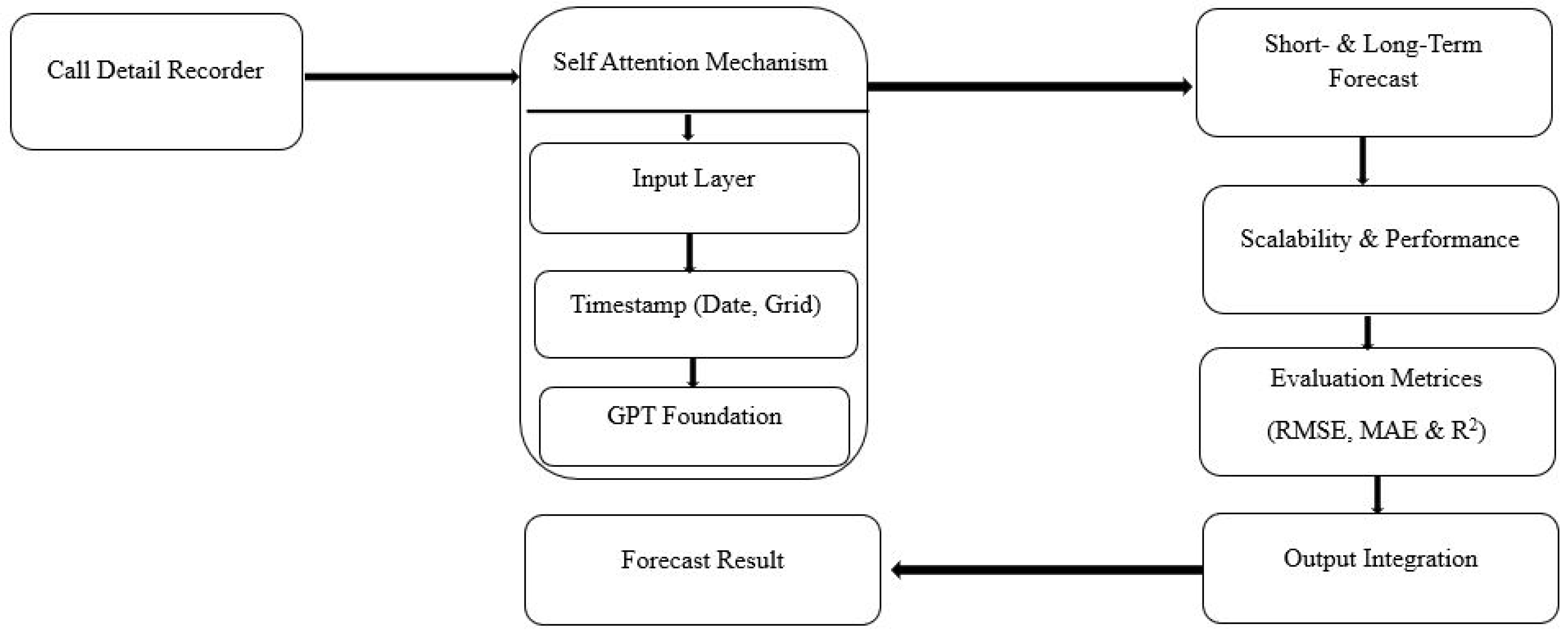
TimeGPT Architecture: The state-of-the-art transformer-based model specifically designed for time series forecasting models addresses the temporal dependencies and provides accurate network traffic forecasts. Figure 2 describes the TimeGPT architecture, which is a transformer-based model for time series forecasting specifically applied to cellular network traffic analysis. It processes Call Detail Records and integrates temporal features such as timestamp, date and grid ID for structured learning. It is built on a GPT-based foundation and uses an integration layer and a self-attention mechanism to capture temporal dependencies. The decoder generates short- and long-term forecasts, providing adaptability. With scalability and performance optimization, the model evaluates forecasting using robust metrics. Lastly, output integration transforms the results into meaningful forecasts, enabling efficient traffic forecasting.

In this study, the architecture is adapted to learn mobile network usage patterns from CDRs. It includes several key steps.

• Input encoding: Raw features such as timestamps, grid IDs and usage metrics are converted into high-dimensional embeddings. Positional encodings are added to preserve the temporal sequence of the inputs.
• Temporal integration layer: Periodic patterns, such as daily or weekly cycles, are captured through additional integrations, allowing the model to learn the seasonality of network behavior.
• Transformer structure: A stacked self-attention mechanism allows the model to learn long-term dependencies over specific time intervals. Multi-head attention further improves its ability to model parallel input relationships.
• Feedback layer: The transformed features are passed through a nonlinear feedback network to enrich the representation.
• Decoder: The model predicts future usage values across a defined forecast horizon (e.g., 24 h), using the contextual embeddings generated in the earlier layers.
• Evaluation Block: The model’s accuracy is validated using standard metrics: RMSE, MAE and R², ensuring both reliability and generalization.

The final output is seamlessly integrated into forecasting pipelines for real-time traffic monitoring, anomaly detection and strategic planning. Each component in TimeGPT plays a distinct role in ensuring that temporal dependencies, seasonal variations and contextual usage shifts are accurately captured. The combination of ProbSparse attention, unidirectional decoding and transformer-based scaling makes this model highly suitable for large-scale mobile network forecasting.

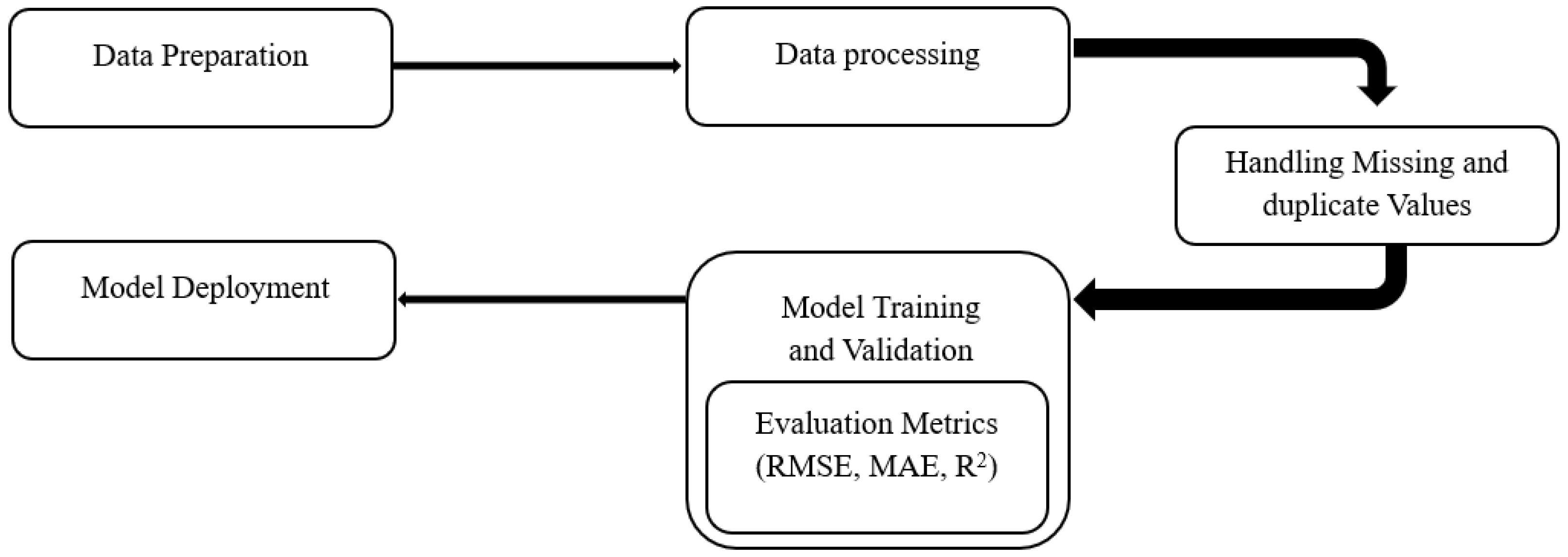
AutoML simplifies and accelerates the model development process by automating key stages such as feature engineering, hyperparameter tuning and model selection. For this study, the H2O AutoML platform was selected due to its strong compatibility with time series data like Call Detail Records (CDRs), which capture temporal and spatial variations in mobile network activity.

The AutoML-based forecasting pipeline, shown in Figure 3, provides a fully automated and scalable approach to processing CDR data, from raw data ingestion to model deployment. The workflow begins with data preparation, which involves cleaning, structuring and formatting raw CDRs. This includes parsing timestamps, normalizing features and encoding spatial identifiers to ensure consistency and interpretability.

A dedicated preprocessing module addresses data quality issues by removing duplicates, filling in missing values and generating important temporal features such as time of day, day of the week and lag indicators. Once preprocessing is complete, the data enters the model training and validation phase. The AutoML engine then runs multiple candidate models in parallel, including Gradient Boosting Machines (GBMs), XGBoost, Random Forests, deep neural networks and stacked ensembles.

During training, H2O AutoML automatically optimizes hyperparameters using advanced techniques such as random grid search and Bayesian optimization to improve model performance. To rigorously evaluate these models, a time series-based cross-validation strategy (step-forward validation) is applied, preserving the temporal sequence and simulating real-world forecasting conditions. Each candidate model is evaluated using standardized performance metrics, including root mean square error (RMSE), mean absolute error (MAE) and R². The model with the best RMSE across all validation criteria is ranked first.

After validation, the best-performing model is deployed for real time forecasting. The pipeline also includes a monitoring mechanism that continuously evaluates forecast performance. If signs of model deviation or degradation, such as increased error rates or changing data patterns, are detected, the system automatically triggers model retraining with the most recent data to ensure high forecast accuracy.

To support this end-to-end workflow, the AutoML pipeline includes several specialized modules.

• Feature Engineering Module: Automatically generates informative predictors, including lag variables, moving averages and spatiotemporal encodings.
• Model Selector: Compares a wide range of algorithms such as Gradient Boosting Machines, XGBoost, deep learning models and stacked ensembles using a ranking mechanism to identify the optimal candidate.
• Hyperparameter Optimizer: Employs techniques like grid search, random search, or Bayesian optimization to fine-tune models for best performance.
• Cross-Validation Engine: Applies time-aware validation methods (e.g., walk-forward validation) to ensure the robustness and generalizability of the selected model.
• Ensemble Module: Optionally blends the predictions of top-performing models to enhance accuracy and reduce variance.
• Forecast Generator: Produces real-time traffic forecasts and supports adaptive learning by triggering model updates based on changing data conditions.

By leveraging H2O AutoML, the entire forecasting pipeline becomes both efficient and interpretable, making it particularly well suited for large-scale, high-frequency, spatiotemporal datasets, such as those used in modern mobile network environments.

Model Evaluation: The forecasting performance of TimeGPT and AutoML was assessed using standard evaluation metrics: mean absolute error (MAE), mean squared error (MSE), root mean square error (RMSE) and the coefficient of determination (R²). To provide a well-rounded analysis, both models were benchmarked against conventional forecasting approaches, including ARIMA, SARIMA and LSTM. These metrics offer a quantifiable measure of predictive accuracy and serve as a consistent basis for comparing the strengths and limitations of each model in capturing the dynamic nature of mobile network traffic.

Model Configuration: To ensure a fair comparison across all models, we standardized the experimental conditions, including data preprocessing, evaluation protocols and parameter tuning. The following configurations were applied:

• TimeGPT (Chronos Library): TimeGPT was implemented using a 24 h sliding window to predict the subsequent 24 h period. Training was conducted with a learning rate of 0.001, a batch size of 32 and a maximum of 50 epochs. Early stopping was applied after five epochs without improvement. Pretrained weights were used to simulate real-world deployment and reduce the need for extensive retraining.
• AutoML (H2O): The AutoML pipeline was configured with a runtime cap of 30 min per run and limited to a maximum of 20 model candidates. RMSE was used as the leader board metric and 5-fold cross-validation ensured the robustness of the results. All preprocessing, feature engineering, model selection and hyperparameter tuning were handled automatically by the H2O AutoML engine, with default settings used for early stopping and random seed to maintain reproducibility.
• Traditional Models:
  ARIMA: Configured with parameters (p = 5, d = 1, q = 0), selected based on AIC minimization and residual analysis.
  SARIMA: Tuned to (p = 1, d = 1, q = 1) (P = 1, D = 1, Q = 0) [using seasonal decomposition and grid search.
  LSTM: Implemented with one LSTM layer (50 units), followed by a dense output layer. The model was trained using the Adam optimizer and MSE loss, with a batch size of 32, dropout rate of 0.2 and 100 epochs.

Fix Model (Model Refinement Strategy): In cases where a model exhibited high training accuracy but underperformed on validation or test data, further optimization was conducted to improve generalization. This included the following:

• Hyperparameter Tuning: Grid search and random search were used to explore various parameter settings for each model.
• Advanced Feature Engineering: Additional features were created based on domain knowledge, including interaction terms and polynomial transformations, to better capture complex patterns.
• Cross-Validation: Models were reevaluated using multiple data splits to ensure consistent performance across different subsets.
• Ensemble Techniques: Where beneficial, ensemble methods such as bagging, boosting, or stacking were applied to combine the strengths of multiple models.

This iterative refinement process continued until the models achieved balanced performance across training and testing phases, indicating readiness for practical deployment in mobile traffic forecasting scenarios.

4. Results and Experimentation

4.1. Correlation Analysis

A correlation map visually represents the strength and direction of relationships between numerical variables. Figure 4 shows the correlation map for the dataset at the specific time interval. It highlights the relationships between different attributes such as incoming/outgoing SMSs, incoming/outgoing calls and data usage. Color-coded cells indicate positive, negative, or no correlation between variables.

Figure 4 presents a correlation matrix generated using Pearson correlation analysis on the preprocessed CDR (Call Detail Record) data. It is important to clarify that this matrix was not derived from a neural network weight matrix but rather constructed to quantify linear dependencies among key telecommunication variables: sms_in, sms_out, call_in, call_outand data_all.

The correlation map in Figure 4 provides a visual representation of the strength and direction of these relationships. Each cell is color-coded to reflect whether the correlation is positive, negative, or negligible. For example, a strong positive correlation (0.83) is observed between sms_in and sms_out, indicating synchronized texting behavior areas with high outgoing SMS activity also tend to receive a high volume of incoming messages. Additionally, the variable data_all shows a moderate positive correlation (0.66) with both call_in and call_out. This suggests that regions with higher mobile data usage also tend to exhibit increased voice call activity, pointing to potential convergence in communication preferences across different services in densely active grid areas.

This correlation analysis helps establish foundational insights into user behavior patterns and supports further modeling and feature selection for predictive tasks.

4.2. Spatial Analysis

After analyzing the correlations, we conducted a spatial analysis of the data by fixing the time and examining the entire city of Milan using CDRs. Figure 5 illustrates the spatial distribution of aggregated CDR activities at a specific timestamp. To simplify the visualization and enable clearer interpretation, we introduced a derived metric termed Combined CDR Activity, calculated by summing all normalized communication metrics: incoming and outgoing calls, SMSs and data usage. The data is plotted on a 100 × 100 spatial grid, with the X and Y axes representing geographic coordinates. Activity levels are represented using a heatmap where color intensity corresponds to usage volume: darker purple shades indicate low activity, while lighter yellow areas signify regions of peak telecom usage. This spatial distribution reveals pronounced activity hotspots in central urban zones likely due to higher population densities and more intensive mobile activity while activity levels diminish in suburban and peripheral areas, reflecting lower population density and reduced communication demand. This visualization offers valuable insight for urban planners and network operators to identify zones requiring infrastructure investment or optimization.

Figure 6 illustrates the temporal progression of spatial CDR usage throughout a single day, using snapshots taken every three hours (00:00, 03:00, 06:00, …, 21:00). This series of heatmaps provides insight into how network activity shifts across the city during daily cycles. The persistence of higher intensity in central regions aligns with working hours and business zones, while peripheral areas show periodic increases, possibly tied to residential routines or commuting.

We further extended our spatial analysis to examine variations across different time slots throughout the day, as shown in Figure 6. These variation maps depict how network activity changes over time, providing insight into usage dynamics throughout the day. Figure 6 presents activity during the complete day at quarterly intervals: 00:00, 03:00, 06:00, 09:00, 12:00, 15:00, 18:00 and 21:00. The analysis shows that central regions consistently experience higher traffic, confirming their status as urban and commercial hubs. In contrast, other regions show fluctuating activity levels depending on the time of day, revealing shifting communication demands.

On the heat maps in Figure 6, dark areas represent grids with the lowest CDR utilization, indicating low network activity. Light areas indicate regions with the highest utilization, often in urban or commercial centers. Moderate or medium colors reflect areas with average or fluctuating activity throughout the day. This color gradient helps visualize the dynamics of communication patterns in different regions and at different times.

4.3. Temporal Analysis

For the temporal analysis, we examined the CDR activity of a specific grid/location over the course of a single day. Figure 7 illustrates the temporal variation in CDR activity. The x-axis represents hourly intervals, while the y-axis shows the level of CDR activity. The figure reveals a distinctive temporal pattern in mobile network usage. Activity is moderate around midnight and gradually declines, reaching its lowest point between 4 a.m. and 6 a.m., a period typically associated with minimal user engagement. A sharp increase in usage begins around 7 a.m., aligning with the start of daily routines, commuting and business communications. The first peak is observed in the early afternoon (around 2–3 p.m.), likely driven by midday internet usage and ongoing work-related activities. The blue line in the figure represents the average usage values per hour and the circular markers indicate the exact data points. Because this figure contains only one data series, no additional color differentiation is applied. The legend field is displayed by default, but does not indicate multiple categories.

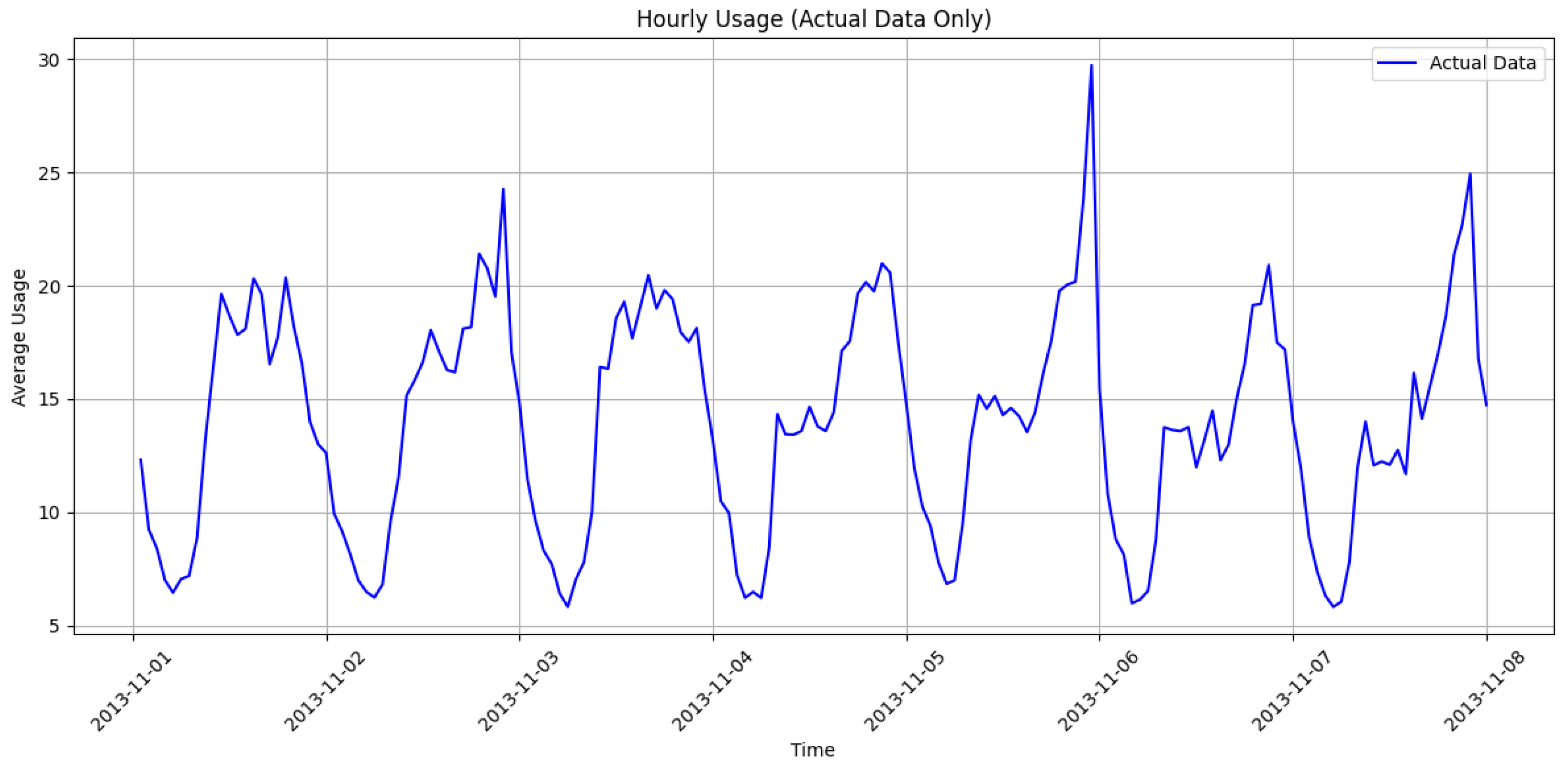
To explore longer-term trends, we analyzed the CDR activity over a one-week period for the same grid. Figure 8 shows the temporal variation in network activity throughout the week. The x-axis represents time in days, while the y-axis shows CDR activity levels. This representation effectively captures usage fluctuations over time. Careful observation reveals a recurring 24 h cycle, indicating that activity closely mirrors human behavioral patterns of higher usage during the day and lower activity at night. The amplitude of these peaks varies across the week, with notable surges on November 3 and 6, possibly due to specific events or anomalies. These trends and outliers are essential for understanding user behavior, optimizing network resources and guiding infrastructure planning.

4.4. Network Traffic Forecasting

After understanding the spatiotemporal variation of the CDR actives, we proceeded to forecast them. For CDR traffic forecasting, we used two different state-of-the-art models: TimeGPT and AutoML.

4.4.1. Traffic Forecasting with TimeGPT

Figure 9 presents the forecasting results of CDR activities generated by the TimeGPT model, using one week of data as the input window. The blue line with circular markers represents the actual average usage, while the dashed red line with cross-markers indicates the predicted values produced by TimeGPT. This side-by-side visualization provides a clear reference point for evaluating the model’s performance in capturing real-world mobile network usage patterns.

The forecasting process involved several key steps to prepare the data and generate predictions. First, the CDR dataset was preprocessed by hourly resampling, handling missing values and normalizing the average application metric to stabilize the learning process. A sliding window approach was then applied to transform the sequential data into a supervised learning framework, where each 24 h input window was used to forecast the next 24 h period. The transformed data was then input into TimeGPT using the Chronos library, which applies a transformer-based temporal architecture to model complex dependencies and periodic patterns. Finally, the results were postprocessed to reverse the normalization and align them with the scale of the original data.

Overall, Figure 9 shows strong agreement between actual and forecasted values throughout the forecast week. Both curves show highly synchronized patterns, with forecasted values closely tracking the peaks and troughs observed during actual usage. This reflects the model’s ability to learn and generalize temporal behavior, capturing the cyclical nature of mobile network usage patterns, such as increased activity during the day and reduced usage in the late evening.

These results highlight the robustness of TimeGPT in modeling dense, high-frequency time series data. The close correspondence between actual and predicted usage indicates that the model effectively internalizes usage dynamics without requiring extensive manual manipulation. While some peak values could benefit from further refinement through external regressors or anomaly correction techniques, the basic forecasting capability remains statistically reliable and operationally efficient.

The evaluation measurements of the TimeGPT model, as shown in

Table 1. Evaluation metrics for the TimeGPT model.

Evaluation Metrix	TimeGPT
RMSE	14.8229
MAE	7.7788
$R^2$	98.62%

, demonstrate its high accuracy and effectiveness in forecasting mobile network traffic. The root mean square error (RMSE) is 14.8229, indicating minimal deviation between actual and forecasted values. The mean absolute error (MAE) is 7.7788, which further reflects the model’s strong predictive accuracy. Additionally, the R² value of 98.62% reflects the excellent model fit that captures nearly all the variability in the data. Overall, these metrics confirm that TimeGPT provides accurate and reliable forecasts, making it a robust tool for mobile network traffic forecasting.

4.4.2. Traffic Forecasting with AutoML

Figure 10 illustrates the forecasting results of CDR activities using the AutoML framework. This prediction covers one week of average mobile network usage. The blue line with circular markers represents the actual observed average usage, while the dashed red line with crosses denotes the predicted values generated by the AutoML pipeline. This visual comparison facilitates a straightforward assessment of how well the automated model aligns with real-world usage trends.

The AutoML forecasting process followed a structured workflow to ensure optimal model selection and tuning. The raw CDR dataset was first aggregated hourly and then cleaned to correct for missing values. The H2O AutoML framework then automated feature engineering steps, including the creation of lag variables, temporal features (such as time of day and day of the week) and trend indicators. The data was split into training and validation sets using a sliding-window cross-validation method to preserve temporal structure. H2O AutoML explored different models, including gradient boosting, deep learning and stacked ensembles. The best performing model was selected based on the root mean square error (RMSE) and used to generate the forecasts. The final predictions were scaled back to their initial values for comparison with actual usage.

As shown in Figure 10, the AutoML model shows a strong correlation between actual average usage and predicted average usage throughout the week. The predicted values effectively track the observed fluctuations, capturing daily peaks and troughs with remarkable accuracy. The alignment of the curves demonstrates AutoML’s ability to automatically extract relevant temporal features and learn usage patterns without manual intervention.

These results reinforce the usefulness of AutoML frameworks for large-scale time-series prediction, particularly in telecom scenarios where data is abundant and rapidly evolving. Despite slight deviations during peak usage, the model displays consistent performance across most time series. This underscores the potential of AutoML as a scalable solution for network operators seeking to anticipate demand and efficiently allocate resources.

The AutoML model evaluation metrics, summarized in

Table 2. Performance metrics for the AutoML model.

Evaluation Metrix	AutoML
RMSE	2.4990
MAE	1.0284
$R^2$	99.96%

, reveal outstanding forecasting performance. The RMSE score of 2.4990 indicates a small average deviation between the actual and forecasted values. The MAE of 1.0284 reflects an even smaller average error size. In addition, the R² value of 99.96% shows an almost perfect model fit, demonstrating its ability to capture virtually all variability in the dataset. These evaluation metrics confirm the strength and reliability of the AutoML model in forecasting mobile network traffic utilization.

An additional analysis revealed that the TimeGPT and AutoML models tend to slightly overestimate periods of high and low usage. This behavior could indicate that they are overfitting to the dominant patterns in the training data, leading to increased sensitivity to extreme values. Furthermore, potential strategies to improve the accuracy of forecasts in extreme cases are discussed that include the development of hybrid modeling approaches. These improvements aim to enhance the robustness of the models and provide promising approaches for future research. This recognition not only increases the transparency of the model evaluation process but also indicates practical ways to improve the overall performance of forecasts.

4.4.3. Hyperparameter Configuration and Tuning Strategy

To ensure optimal performance and a fair comparison, both TimeGPT and AutoML models were configured with clearly defined strategies tailored to their respective architectures. While TimeGPT relies on a pretrained transformer network via the Chronos framework, AutoML leverages H2O’s automated pipeline to find the best model and parameters with minimal manual intervention.

Table 3. Comparison of TimeGPT (Chronos) and AutoML (H2O framework).

Parameter	TimeGPT (Chronos)	AutoML (H2O Framework)
Input Window	24 h	24 h
Forecast Horizon	24 h	24 h
Learning Rate	0.001 (default)	Random grid search
Batch Size	32	Auto Selected per Model
Epochs	50	Determined per Model
Pretrained Weights	Used	Not Applicable
Cross-Validation	Not applied	Five-Fold Time-Series-Aware CV
Model Candidates	Single	Max 20 models
Hyperparameter Tuning	Skipped	Random Grid Search
Ensemble Methods	Not used	Stacked Ensembles
Feature Engineering	Positional Encoding	Automated

presents a consolidated overview of the main hyperparameter configurations for both models. TimeGPT was configured with an input window and a forecast horizon of 24 h. A batch size of 32 and a maximum of 50 training periods were used, with early stopping after five consecutive periods without improvement. The learning rate was kept at the default value of 0.001 and transfer learning was performed with pretrained weights to minimize the need for manual tuning. Chronos handles most of the optimization internally, eliminating the need for manual hyperparameter tuning.

A more dynamic and fully automated workflow was introduced for AutoML. The H2O framework autonomously performed feature engineering, model selection and hyperparameter tuning using random grid search strategies. Each candidate model was given a maximum run time of 120 s and the system evaluated up to 20 models using five fold time series cross-validation. Different algorithms were explored, including Gradient Boosting Machines, XGBoost, Random Forests, deep learning and stacked ensembles, with automatic selection of the best performing model based on RMSE.

As summarized in Table 3, the two models differ significantly in their handling of feature tuning and engineering. TimeGPT’s pipeline emphasizes the efficiency of the pretrained architecture, while AutoML optimizes predictive performance through extensive automated exploration.

5. Discussion and Comparison

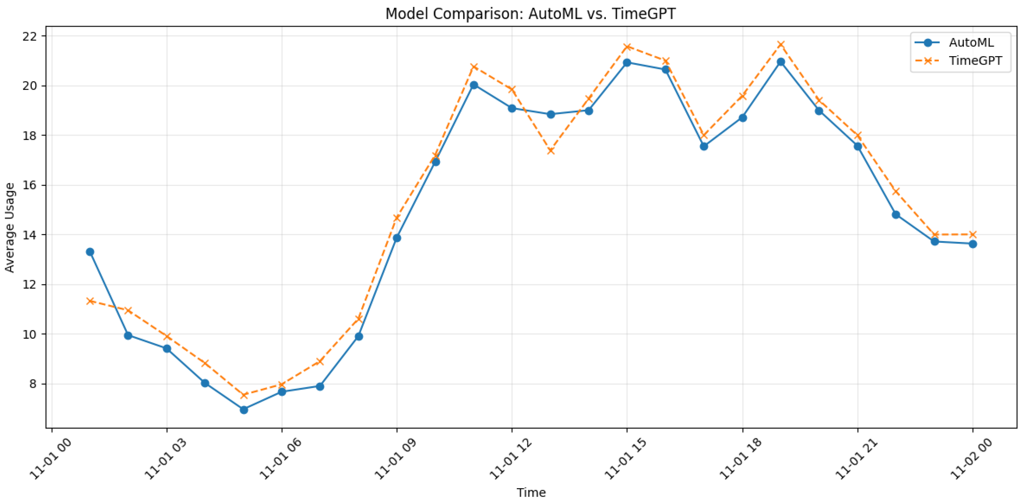
TimeGPT and AutoML offer distinct capabilities for mobile network traffic forecasting, each excelling in different areas. TimeGPT is specifically designed for time series data, making it highly effective at capturing and forecasting complex patterns in large, dynamic datasets. However, in terms of absolute accuracy, TimeGPT exhibits slightly higher error values compared to AutoML.

Figure 11 illustrates a comparative analysis of the average 24 h usage profiles for two predictive models: AutoML and TimeGPT. The x-axis represents the time in hourly intervals since November 1st with the time change, while the y-axis shows the average usage values. The AutoML model is represented by a solid blue line and circle markers, while the TimeGPT model is represented by a dashed orange line and x markers. Both models show a similar usage pattern throughout the day, with a decrease in usage in the early morning (around 5:00 to 6:00 a.m.), followed by a steady increase from 8:00 a.m., reaching maximum values between 1:00 p.m. and 4:00 p.m. and gradually decreasing around midnight. Notably, TimeGPT shows slightly higher average usage during peak hours, suggesting better responsiveness or adoption during high demand. The close alignment of the two curves during most of the day indicates that both models perform similarly in tracking and predicting usage patterns, with TimeGPT showing marginal advantages during peak hours. This comparison underscores the reliability and effectiveness of both models in time-sensitive applications while also highlighting TimeGPT’s potential advantage in handling more intense usage scenarios.

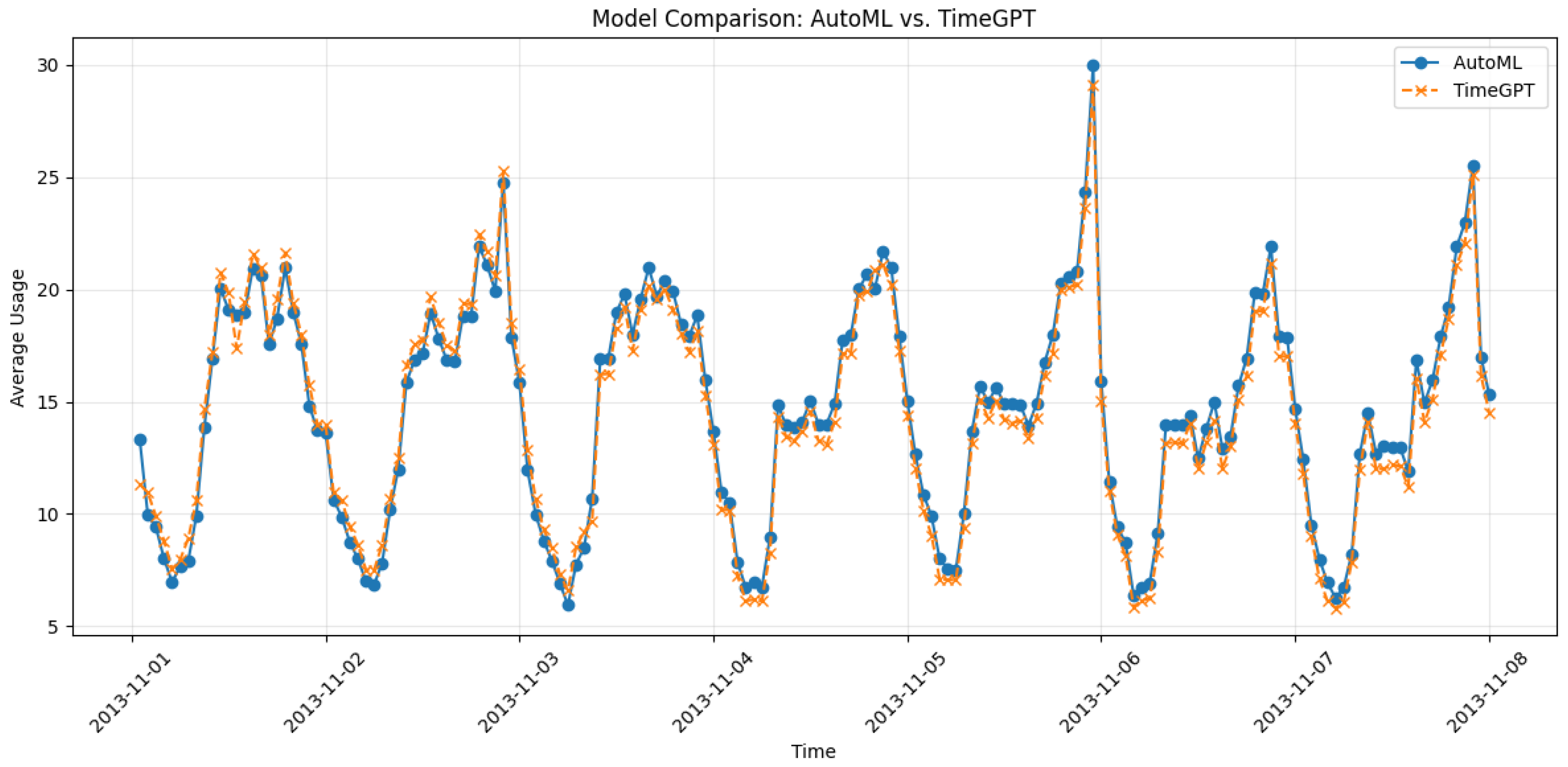
Figure 12 illustrates a time series comparison of the average utilization predictions of the AutoML and TimeGPT models from 1 to 8 November 2013. The x-axis represents the dates, while the y-axis shows the average utilization values. Both models display similar temporal patterns, capturing daily cycles and fluctuations in utilization. It is notable that they respond effectively to rapid changes, such as the sharp spike observed on November 6. TimeGPT sometimes exhibits slightly higher or earlier spikes than AutoML, indicating slightly stronger sensitivity to changes. Despite these slight differences, the overall trends produced by the two models are closely aligned. This similarity suggests that both models are reliable for forecasting or modeling utilization over time. TimeGPT’s subtle advantage in responsiveness might make it slightly more suitable for scenarios involving rapid or frequent variations.

We compared TimeGPT and AutoML to traditional statistical models such as ARIMA, SARIMA and LSTM, and TimeGPT and AutoML significantly outperformed them. Figure 13, titled “Mobile network usage: actual forecasts and model forecasts (day-1 records),” illustrates a comparative analysis of several forecasting models using actual mobile network usage data on 1 November. The actual usage trend is represented by a solid black line, which serves as a benchmark to evaluate the accuracy of five predictive models: ARIMA (blue dotted line), SARIMA (green dotted line), LSTM (red dotted line), AutoML (blue dotted line) and TimeGPT (orange dotted line). Over 24 h, all models attempt to capture the daytime usage pattern with varying degrees of accuracy. Notably, TimeGPT and AutoML closely follow the actual utilization curve, effectively capturing morning troughs and evening peaks, suggesting high adaptability to short-term fluctuations. In contrast, ARIMA and SARIMA exhibit more pronounced deviations, especially during transition hours, indicating limitations in handling nonlinear and seasonal trends. The LSTM model exhibits smoother transitions but tends to underestimate expectations during peak hours, likely due to its reliance on historical smoothing. This comparison highlights TimeGPT and AutoML as the most reliable models for real-time mobile network demand forecasting, demonstrating their potential usefulness in network management and resource allocation strategies.

Figure 14, “Mobile network usage: models comparison (actual vs. TimeGPT vs. AutoML vs. ARIMA vs. SARIMA vs. LSTM)”, provides a detailed comparative analysis of six forecasting models in predicting average mobile network usage over the period from 1 to 8 November 2013. The actual observed data is represented by a bold black line, serving as the benchmark against which the predictive accuracy of the models: ARIMA (blue dashed), SARIMA (orange dashdot), LSTM (green dotted), AutoML (red solid) and TimeGPT (purple dashed) are assessed. All models generally succeed in capturing the underlying daily patterns and periodic surges in network usage, reflecting a shared ability to model cyclical behavior. However, TimeGPT and AutoML exhibit the closest alignment with the actual data, especially during peak demand periods and abrupt fluctuations, suggesting superior sensitivity and forecasting precision. In contrast, ARIMA and SARIMA tend to underperform during rapid changes, often over or underestimating peak values. The LSTM model provides smoother forecasts but occasionally lags in responsiveness, potentially missing finer temporal variations. Notably, the consistent proximity of TimeGPT and AutoML to the actual usage line underscores their robustness and adaptability in complex, time-variant environments. This comparative visualization highlights TimeGPT and AutoML as the most effective models among those evaluated, making them strong candidates for real-time network demand forecasting applications.

As shown in

Table 4. Comparison of forecasting performance metrics across various models.

Evaluation Metrix	RMSE	MAE	R2
AutoML	2.4990	1.0284	99.96%
TimeGPT	14.8226	7.7789	98.62%
ARIMA	10.8205	9.1472	83.80%
SARIMA	15.1946	13.1610	60.76%
LSTM	9.6017	9.6017	79.3%

, the RMSE for TimeGPT is 14.8226 and the MAE is 7.7789, while AutoML performs significantly better with an RMSE of 2.4990 and an MAE of 1.0284. This suggests that AutoML produces more accurate forecasts with lower deviations from actual values. Additionally, the R² value, which measures how well the model explains the variance in the data, shows a crucial difference: AutoML achieves an impressive R² of 99.96%, indicating near-perfect predictive power, while TimeGPT scores 98.62%, which is strong but slightly lower, as shown in Table 4. This reinforces AutoML’s superior forecasting accuracy.

This study sets a new benchmark in mobile traffic forecasting by demonstrating that the proposed models AutoML and TimeGPT significantly outperform traditional forecasting approaches such as ARIMA, SARIMA and LSTM. As detailed in Table 4, conventional statistical models exhibit notable limitations: ARIMA yields a moderate R² of 83.80% with RMSE and MAE scores of 10.8205 and 9.1472, respectively; SARIMA performs even more poorly with an R² of just 60.76%, with RMSE and MAE scores of 10.8205 and 9.1472, respectively, highlighting its inability to capture the complex spatiotemporal dynamics of mobile network data. Although LSTM shows slight improvement with an R² of 79.3%, its results lack consistency and robustness.

By contrast, the integration of TimeGPT and AutoML represents a novel methodological leap in forecasting accuracy and model efficiency. TimeGPT, with its transformer-based architecture, is purpose-built for time series forecasting and excels at learning intricate temporal dependencies, seasonalities and irregular fluctuations. AutoML, on the other hand, delivers a fully automated modeling pipeline, including feature engineering, algorithm selection and hyperparameter optimization, enabling high-performance forecasting with minimal human intervention.

The empirical results clearly favor AutoML as the best-performing model, with a near-perfect R² of 99.96%, the lowest RMSE 2.4990 and the lowest MAE 1.0284. TimeGPT follows closely with a solid R² of 98.62%, demonstrating its robustness in capturing temporal trends. The novelty of this work lies not only in the systematic application of these advanced tools to mobile traffic prediction but also in setting a new standard through rigorous comparative evaluation. Moreover, the study proposes a promising hybrid strategy that combines the temporal modeling advantages of TimeGPT with the automation of AutoML to provide a scalable, accurate and generalizable prediction framework, laying the foundation for future research in intelligent network planning.

In conclusion, both TimeGPT and AutoML offer unique advantages for time series forecasting: AutoML excels in its high overall accuracy, while TimeGPT is particularly effective at capturing complex temporal patterns. A hybrid approach leveraging both could result in a robust forecasting framework, combining predictive accuracy with nuanced temporal understanding.

6. Conclusions

This study proposed a data-driven mobile traffic analysis and forecasting framework using Telecom Italia’s Call Detail Records (CDRs). By dividing Milan into a detailed 100 × 100 grid and categorizing traffic into four intensity levels, we captured the spatial and temporal dynamics of network demand across the city. The analysis revealed that high traffic concentrations are mainly located in central urban areas, highlighting the influence of population density and mobility patterns. To evaluate the prediction performance, AutoML and TimeGPT were used to predict traffic trends. While TimeGPT effectively captured complex temporal dependencies, AutoML consistently achieved higher accuracy and demonstrated greater adaptability. Its automated pipeline, including feature selection and model tuning, made it a more practical solution for real-world telecom applications. These results highlight the considerable potential of AutoML for intelligent and scalable network management, particularly in the context of smart city infrastructures. Future research could benefit from incorporating additional contextual data (such as weather conditions, special events, or travel patterns) to improve forecast accuracy. Testing the proposed models in multiple cities and over longer time periods would assess their robustness and generalizability. Furthermore, integrating privacy preserving techniques, such as federated learning, could enable broader collaborative use without compromising user data. A hybrid approach combining the temporal modeling strengths of TimeGPT with AutoML optimization could also offer a promising direction. Finally, evaluating the model’s performance in various urban environments will be essential to validate its adaptability and ensure its practical deployment in various real-world scenarios.