A Novel MaxViT Model for Accelerated and Precise Soybean Leaf and Seed Disease Identification

Abstract

Timely diagnosis of soybean diseases is essential to protect yields and limit global economic loss, yet current deep learning approaches suffer from small, imbalanced datasets, single-organ focus, and limited interpretability. We propose MaxViT-XSLD (MaxViT XAI-Seed–Leaf-Diagnostic), a Vision Transformer that integrates multiaxis attention with MBConv layers to jointly classify soybean leaf and seed diseases while remaining lightweight and explainable. Two benchmark datasets were upscaled through elastic deformation, Gaussian noise, brightness shifts, rotation, and flipping, enlarging ASDID from 10,722 to 16,000 images (eight classes) and the SD set from 5513 to 10,000 images (five classes). Under identical augmentation and hyperparameters, MaxViT-XSLD delivered 99.82% accuracy on ASDID and 99.46% on SD, surpassing competitive ViT, CNN, and lightweight SOTA variants. High PR-AUC and MCC values, confirmed via 10-fold stratified cross-validation and Wilcoxon tests, demonstrate robust generalization across data splits. Explainable AI (XAI) techniques further enhanced interpretability by highlighting biologically relevant features influencing predictions. Its modular design also enables future model compression for edge deployment in resource-constrained settings. Finally, we deploy the model in SoyScan, a real-time web tool that streams predictions and visual explanations to growers and agronomists. These findings establishes a scalable, interpretable system for precision crop health monitoring and lay the groundwork for edge-oriented, multimodal agricultural diagnostics.

1. Introduction

Soybean is an essential crop serving as a primary source of protein and oil for human consumption and animal feed. It accounts for nearly 60% of global oilseed production [1]. In 2023, the soybean market was valued at over USD 160 billion, with a projected compound annual growth rate (CAGR) of 4.4% from 2024 to 2030  [2,3]. The United States, Brazil, and Argentina collectively contribute more than 80% of the world’s soybean production, highlighting the crop’s importance for food security and international trade [4]. However, soybean cultivation faces significant challenges due to various diseases affecting both leaves and seeds. 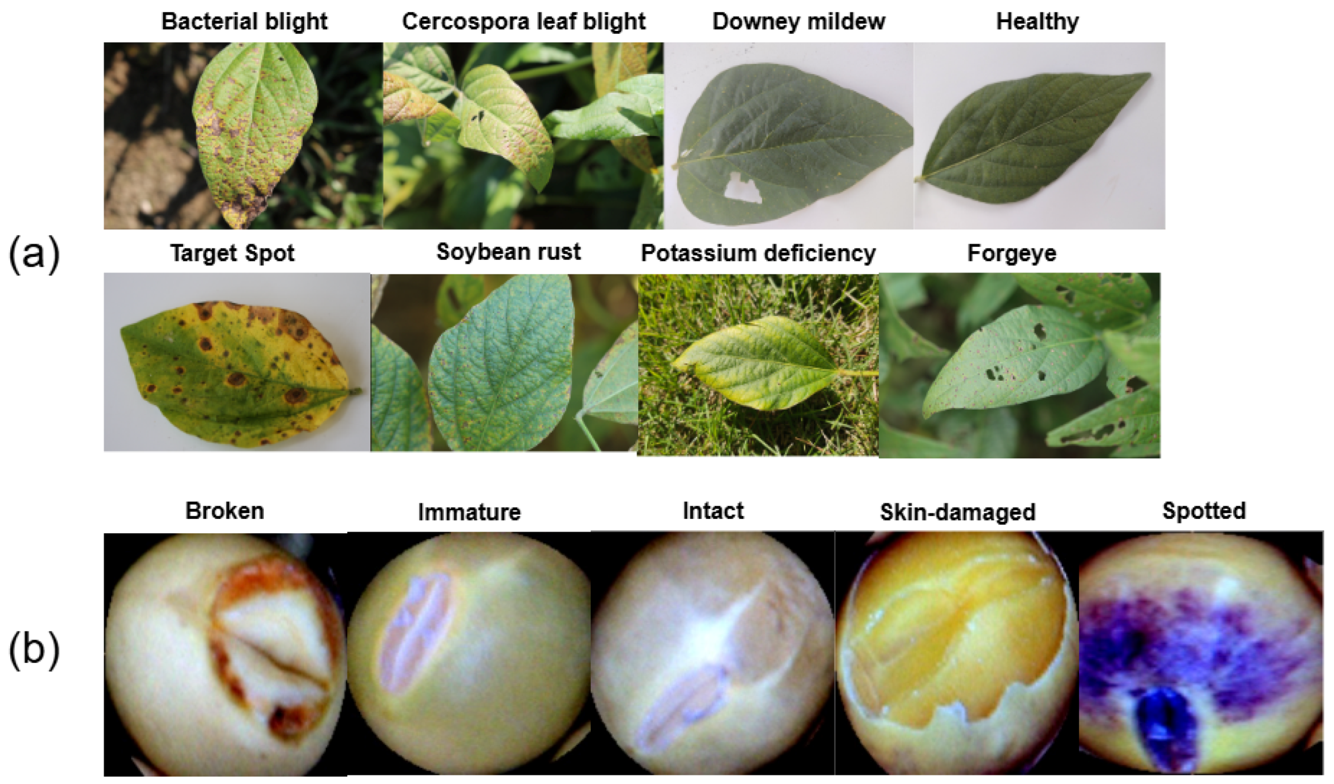These diseases can lead to yield losses of up to 30% annually, resulting in USD billions in economic losses worldwide [5,6]. Common diseases include bacterial blight, Cercospora leaf blight, and frogeye leaf spot, along with seed-specific defects such as skin damage and immaturity [7]. These issues not only reduce yield but also compromise product quality, which impacts market value and food security [8]. Timely and accurate detection of these diseases is critical for implementing effective disease management strategies and mitigating yield losses [9]. Traditionally, disease diagnosis relies on manual inspection by agricultural experts. While this approach has been effective in small-scale applications, it is labor-intensive, time-consuming, and prone to human error, particularly in large-scale agricultural operations [10,11]. Furthermore, visual inspection often fails to accurately identify early-stage infections or subtle disease symptoms, leading to delayed interventions. These limitations highlight the need for automated, reliable, and scalable solutions [12].

Deep learning models, such as convolutional neural networks (CNNs), show outstanding performance in the detection of plant diseases [13]. Transfer learning enhances CNNs in agriculture by fine-tuning pretrained models for specific applications [14]. However, there are still difficulties due to small, imbalanced datasets that prevent them from generalizing to real-world scenarios. Combining the predictions from multiple models into an ensemble model results in the models often outperforming individual CNNs because of the increase in robustness, accuracy, and generalizability. Bagging, boosting, and stacking reduce overfitting and handle noisy data better [15]. However, they suffer from high cost for both training and inference and lack interpretability since they consider many models. On the other hand, ViTs provide a unified and scalable architecture that can bypass this and does not require multiple models. The self-attention mechanism of ViTs is able to sufficiently capture the local and global dependencies so that they are able to effectively generalize even when few data are available [16]. Also, they offer better explainability through attention maps, making them more efficient and interpretable for complex datasets.

While progress has been made in the field of soybean disease classification, there are notable gaps. Most studies focus only on soybean leaf diseases or seed defects, lacking a unified framework for both. This limits the scalability and comprehensiveness of existing approaches. ViTs have shown promise in various tasks, but their potential for soybean diagnostics, particularly for leaf and seed datasets, has not been thoroughly explored. Many existing studies report high classification accuracy on limited datasets but fail to provide rigorous validation and performance analysis. Additionally, current deep learning models often operate as black boxes, offering little transparency. Few studies utilize explainable AI tools to identify key features influencing predictions and practical solutions.

This study aims to fill research gaps by creating a strong, clear, and scalable framework for classifying soybean diseases. The specific objectives are as follows:

• Develop a framework to accurately classify diseases affecting soybean leaves and seeds.
• Identify the most effective ViT-based architecture that effectively captures both global and local features.
• Achieve state-of-the-art performance on multiple datasets for disease identification over existing studies.
• Develop a trustworthy web-based application designed to support agricultural professionals.

To achieve our objectives, we developed a framework for classifying soybean leaf and seed diseases using MaxViT models on various datasets. Among the various ViT architectures, MaxViT was selected due to its hybrid design, which combines convolutional layers with multiaxis self-attention. This design allows MaxViT to effectively capture both local features (texture, color, and edges) and global spatial patterns present in whole-leaf or seed images. In contrast to standard ViTs, which may overlook fine-grained details or require significant computational resources, MaxViT provides a balanced trade-off between accuracy, efficiency, and interpretability. This makes it particularly suitable for agricultural diagnostics. Although MaxViT is a recognized architecture, this study is the first to apply it in a unified framework for classifying both soybean leaf and seed diseases. Its performance is further enhanced through dataset-specific augmentation, Grad-CAM-based interpretability, and real-time deployment via the SoyScan web platform. 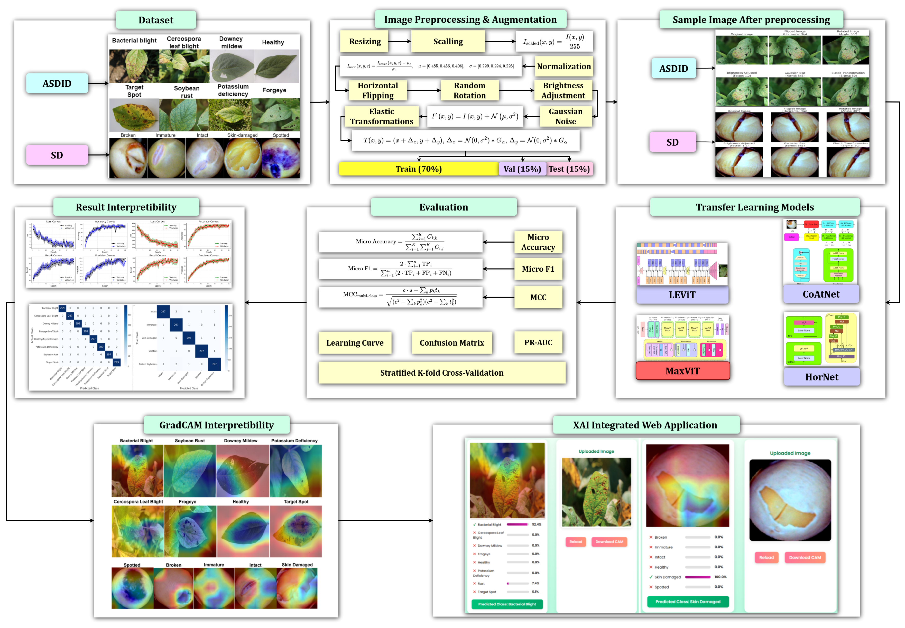Figure 1 illustrates the complete workflow of the proposed methodology. Our contributions include the following:

• We developed an interpretable approach for accurately recognizing diseases in soybean leaves and seeds.
• We proposed an efficient MaxVit-XSLD model that considers both local and global features for soybean disease classification.
• We conducted a comparative performance analysis of various models, providing statistical proof that our method outperforms existing approaches.
• We developed a web application for specialists to improve transparency in the global food security and disease management sectors.

The remainder of this paper is organized as follows: Section 2 reviews related works, with a focus on transfer learning, ensemble methods, and ViTs. Section 3 describes the datasets, preprocessing techniques, and deep learning architectures utilized in this study. Section 4 presents the experimental results and their analysis, while Section 5 discusses the implications and limitations of the findings. Finally, Section 6 concludes this paper and outlines future research directions.

2. Related Works

Deep learning has significantly improved plant disease classification using CNNs and ViTs. While previous studies on soybean health have concentrated on either leaf or seed disease detection, they primarily relied on transfer learning-based CNNs. Although these models achieve high accuracy, they often face issues like poor generalizability, limited interpretability, and challenges in practical deployment. Additionally, soybean seed disease classification is still largely unstudied, and few models integrate both leaf and seed detection. This section reviews the shift from CNNs to ViTs in deep learning approaches and highlights the need for the proposed MaxViT-XSLD model to address these gaps.

2.1. Soybean Leaf Disease Identification

Several studies have applied traditional CNNs for soybean leaf disease classification using transfer learning. For instance, Farah et al. [17] utilized VGG19 for the binary classification of 6410 soybean leaf images, distinguishing between healthy leaves and those infested with Diabrotica speciosa or caterpillars. Their model achieved an accuracy of 93.71%, but it faced limitations due to dataset imbalance and a lack of external validation. Goshika et al. [18] developed a YOLOv5-based model that reached 92% accuracy on 2930 images, focusing on classifying the severity of leaf damage. Although they improved the model through data augmentation and automated labeling, it struggled with occlusions and overlapping leaves in real-world field conditions.

Bevers et al. [19] employed DenseNet201 to classify 10,722 images across eight soybean disease classes, achieving an accuracy of 96.8%. However, high background variability and limited diversity within the dataset hampered generalization. Yu et al. [20] proposed TRNet18, an enhanced ResNet18 model that classified four disease types using 53,250 augmented images derived from 726 originals. This model implemented advanced preprocessing techniques, including image registration and OTSU-based segmentation, resulting in an impressive accuracy of 99.53% and a Macro-F1 score of 99.54%. Despite these accomplishments, it exhibited misclassification tendencies due to overlapping disease symptoms and image distortions.

Their subsequent work, RANet18 [21], introduced residual attention layers with channel and spatial modules in a lightweight network, achieving 96.50% accuracy on 4301 augmented images from 523 samples. While this model proved efficient, it faced challenges with mixed infections and low-quality field samples. Other notable CNN-based contributions include Hang et al. [22], who combined ConvLSTM, squeeze-and-excitation (SE) blocks, and Choquet fuzzy ensembles to achieve 94.27% accuracy on 2820 augmented images. However, they still encountered difficulties in detecting mild symptoms and addressing dataset imbalance.

Song et al. [23] introduced DDC-P, a biologically inspired cell P system that integrated SGEFA, EFA, and fuzzy control for structural optimization of their model. They achieved 98.43% accuracy on a custom dataset and 94.40% on the Auburn dataset, although performance diminished when faced with indistinct visual symptoms. Pan et al. [24] presented TFANet, a two-stage feature aggregation framework employing TFA, DCFF, and InceptionC modules on the ASDID dataset, which contained 20,951 augmented images. The model achieved 98.18% accuracy and a Macro-F1 score of 98.39% while maintaining only 1.18 million parameters, surpassing ResNet and DenseNet. However, its lack of field deployment restricts evaluation under complex agricultural conditions. Sharma et al. [25] introduced SoyaTrans, a hybrid Swin Transformer-CNN model for fine-grained classification. Trained on 4829 real-field images across six classes and four public datasets (PlantVillage, PlantDoc, AI2018, Embrapa), the model achieved 94% accuracy on real-world data and up to 98% on benchmark datasets. It employed random shifting to reduce computational complexity but struggled with small lesion regions and cluttered backgrounds.

Shahzore et al. [26] proposed a pure ViT framework evaluated on three datasets— Auburn, Soybean Diseased Leaf, and SoyNet—achieving accuracies of 98.7%, 98.9%, and 97.4%, respectively. While this model outperformed CNN-based baselines, it may face generalization issues in diverse environments due to its reliance on labeled training data. Wang et al. [27] constructed a Swin Transformer-based model to detect five disease stages (background, normal, early, middle, late) using 15,600 augmented images. With the application of a Sliding Segmentation Algorithm and transfer learning from six CNNs and Transformers, the model achieved 99.64% accuracy and F1 score. Nonetheless, the artificial infection-based dataset and laboratory conditions limit its real-world applicability.

Yu et al. [28] addressed data scarcity with a GAN-based enhancement pipeline, utilizing a cyclic generative adversarial network (cGAN) and a dense-connected discriminator. The resulting synthetic dataset featured nine disease classes and yielded a ViT model accuracy of 95.84%, although concerns regarding real-world variability persist. Wu et al. [29] further extended ConvNeXt by incorporating a CBAM attention mechanism, achieving an accuracy of 85.42% on 11,655 images. However, the model was computationally intensive and struggled with similar lesion features.

2.2. Soybean Seed Disease Classification

Compared to leaf-based studies, soybean seed disease classification remains relatively underexplored in the literature. Most existing studies focus on defect detection, seed quality estimation, or varietal classification, often using CNN-based models and specialized imaging modalities. Zhang et al. [30] developed a deep learning model using AlexNet on UAV imagery to detect soybean seedling emergence, achieving a high accuracy of 99.92% on 12,000 images. While promising, the model was sensitive to lighting variations and did not address disease or defect classification. Sable et al. [31] introduced SSDINet, a lightweight CNN model incorporating Seed Contour Detection (SCD) and SE blocks for efficient seed defect recognition. Trained on a custom dataset of 1000 images across eight classes (one healthy, seven defective types), SSDINet reached 98.64% accuracy. However, the model’s generalization is limited due to the dataset’s small size and regional specificity.

Zhang et al. [32] further proposed DAFFnet, a Dual Attention Feature Fusion Network combining 3D/2D CNNs with CBAM and Mobile Vision Transformer (MViT) modules to classify hyperspectral images of soybean seed varieties. On 4600 images (across 20 varieties), DAFFnet achieved 96.15% accuracy, outperforming baseline models. However, its complexity and use of hyperspectral inputs pose scalability and deployment challenges. Yang et al. [33] explored RGB reconstruction of hyperspectral images to classify 7616 seed samples from seven soybean classes. Their best model, SENet-ResNet34-DCN, achieved 94.24% accuracy, but visually similar varieties (e.g., H1 vs. H6) and limited dataset diversity constrained performance.

Dioses et al. [34] used EfficientNet-B0 to classify seed quality across five categories (broken, immature, intact, skin-damaged, spotted) using 5000+ images. The model reached 93.83% validation accuracy and a 97.35% F1 score for intact seeds. Nonetheless, misclassifications between visually similar categories (e.g., broken vs. spotted) highlighted limitations in feature separability. Lin et al. [35] introduced SoyNet, a real-time seed classification system built on a lightweight CNN trained on 3100 images (four classes). With MSRCR-based preprocessing and optimized for NVIDIA Jetson TX2, SoyNet achieved 95.63% accuracy with an average inference time of 4.92 ms. While efficient, performance dropped for non-classifiable seeds, and dataset scale limited robustness.

Other innovative approaches include Miranda et al. [36], who implemented a morphological trait-based phenotyping system to predict hundred-seed weight (HSW) from 234,000 seeds spanning 275 genotypes. Using CNNs (ResNet-50) and traditional ML algorithms (MLP, SVR), they achieved an accuracy of 0.71 under varied environmental conditions. However, biotic stress factors, such as rust infection, introduced variability that affected prediction consistency. Chen et al. [37] employed Spatial Frequency Domain Imaging (SFDI) and Reinforcement Learning-optimized SVM (RL-SVM) to classify 300 soybean seeds into mild, moderate, or severe pest-damaged categories. The model reached 98.83% accuracy and 96.35% macro-Recall but required expensive hardware and lacked support for different seed colorations.

Kaler et al. [38] presented a ConvLSTM-based framework using laser bio-speckle imaging to detect fungal infections. Their model achieved 97.72% (binary) and 99% (multiclass) accuracy across 600 samples. While robust against noise, the setup relied on synthetic extension and specialized imaging tools, reducing its real-world applicability. Despite these efforts, no existing study has applied ViT-based architectures for soybean seed disease classification. Most works utilize CNNs with either handcrafted features or hyperspectral data, often constrained by dataset limitations, model complexity, or hardware requirements.

2.3. Limitations of Existing Works

Current research on soybean disease detection faces several key limitations. Most models focus on either leaf or seed diseases, limiting their practical use. Many studies utilize small, imbalanced, or homogeneous datasets, which affects model generalization across different conditions. Additionally, there is a lack of interpretability in many works, as few use explainable AI methods like GradCAM, undermining transparency and user trust. While some models achieve high accuracy, they often lack real-time, user-friendly deployment options for web or mobile use. Moreover, many high-performing models require substantial computational resources, making them unsuitable for field-level application. To address these issues, the MaxViT-XSLD architecture was developed, which classifies both soybean leaf and seed diseases within a unified framework. It is trained on two balanced datasets and incorporates GradCAM-based interpretability to enhance decision-making transparency. MaxViT-XSLD is also deployed through the SoyScan web application, offering real-time diagnostics for agricultural use.

3. Proposed Methodology

3.1. Data Description

We used ASDID [19] and SD [39] multiclass datasets for leaf and seed disease classification, respectively. ASDID contains 10,722 images of soybean leaves, categorized into eight distinct classes: bacterial blight (1072 images), Cercospora leaf blight (1636 images), downy mildew (756 images), frogeye leaf spot (1650 images), healthy/asymptomatic (1663 images), potassium deficiency (1083 images), soybean rust (1754 images), and target spot (1108 images). These images were collected during the 2020 and 2021 growing seasons at various agricultural research stations in Alabama, USA, including the EV Smith Agricultural Research Station and the Brewton Agricultural Research Unit. Two devices were used for image acquisition: a Canon EOS 7D Mark II DSLR camera and a Motorola Moto Z2 Play smartphone. Approximately 70% of the images were taken in the field, showing soybean leaves still attached to the plant, while the remaining 30% featured detached leaves photographed on trimmed grass or a white surface. To ensure diversity in the dataset, images were captured under varying light conditions, including full sunlight and shade, and included leaves at different heights and positions. A detailed class distribution of the ASDID dataset is presented in

Table 1. Class distribution of the ASDID dataset across eight disease categories.

Disease Category	Number of Images
Bacterial blight	1072
Cercospora leaf blight	1636
Downy mildew	756
Frogeye leaf spot	1650
Healthy/asymptomatic	1663
Potassium deficiency	1083
Soybean rust	1754
Target spot	1108
Total	10,722

.

The SD dataset consists of 5513 images of individual soybean seeds, categorized into five categories: intact, immature, skin-damaged, spotted, and broken. These categories were defined based on the Standards of Soybean Classification (GB1352-2009) [40] to ensure consistency and relevance to real-world applications. Each category contains over 1000 images: 1201 images of intact soybeans, 1125 images of immature soybeans, 1127 images of skin-damaged soybeans, 1058 images of spotted soybeans, and 1002 images of broken soybeans. The images of soybean seeds were captured using an industrial camera under controlled conditions. The camera was positioned 143 mm away from the soybeans and was equipped with a uniform light source providing an intensity of approximately 2000 Lux. The class distribution of the SD dataset is detailed in

Table 2. Class distribution of the SD dataset, categorized into five classes.

Disease Category	Number of Images
Intact	1201
Immature	1125
Skin-damaged	1127
Spotted	1058
Broken soybeans	1002
Total	5513

. Figure 2 illustrates different disease and defect categories for soybean leaves and seeds from the ASDID and SD datasets.

3.2. Data Preprocessing and Augmentation

To prepare the datasets for training, all images were first resized to a uniform resolution of 224 × 224 pixels. This resizing step ensured consistency across the datasets, reduced computational complexity, and preserved essential visual features. Standardizing the image dimensions was crucial to align the input data with the selected architectures and optimize model performance.

Following resizing, pixel values were scaled to a range of $[0,1]$, and further normalization was applied using ImageNet statistics (mean values: [0.485, 0.456, 0.406] and standard deviations: [0.229, 0.224, 0.225]). Normalization helped standardize the input data distribution, aligning it with the pretrained weights of the models. This step improved training efficiency and facilitated faster convergence [41].

To address class imbalances and enrich dataset diversity, augmentation techniques were applied to the entire dataset prior to splitting. These techniques included horizontal flipping (50% probability), random rotation $\pm {30}^{\circ }$, brightness adjustment (up to $\pm 10\%$), Gaussian noise, and elastic transformations. Gaussian noise can simulate real-world imperfections in image acquisition, such as sensor noise or environmental factors [42]. It was selected to simulate sensor-induced disturbances, background clutter, and illumination inconsistencies that frequently affect image acquisition in uncontrolled environments. This form of perturbation forces the model to learn robust feature representations by training on images with subtle noise variations, reducing overfitting and increasing tolerance to noise during inference. Prior studies [43,44] have shown that adding Gaussian noise during training improves the model’s resilience to corrupted inputs and enhances generalization in deployment settings. The noise was generated using (Equation (1)), where $I(x,y)$ is the pixel value at location $(x,y)$, $I^{\prime }(x,y)$ is the new pixel value after adding noise, and $\mathcal{N}(\mu ,{\sigma }^2)$ represents Gaussian noise with mean ($\mu =0$) and variance (${\sigma }^2$). The variance was adjusted to ensure the noise introduced thin yet realistic variations without overwhelming the original image.

$$I^{\prime }(x,y)=I(x,y)+\mathcal{N}(\mu ,{\sigma }^2)$$

(1)

Elastic transformations (ETs) were chosen for their ability to mimic realistic, non-rigid deformations such as leaf curling, bending, or seed warping—phenomena commonly observed in plant phenotyping [45]. These transformations used displacement fields to locally warp the image, defined as Equation (2), where $(x,y)$ is the original pixel position and $({\Delta }_x,{\Delta }_y)$ are displacement fields generated by convolving random noise with a Gaussian filter (Equation (3)). $G_{\sigma }$ is a Gaussian kernel with standard deviation ($\sigma$), controlling the smoothness of the deformation.

$$T(x,y)=(x+{\Delta }_x,y+{\Delta }_y)$$

(2)

$${\Delta }_x=\mathcal{N}(0,{\sigma }^2)\ast G_{\sigma },{\Delta }_y=\mathcal{N}(0,{\sigma }^2)\ast G_{\sigma }$$

(3)

ET was first introduced by Simard et al. [46] and has since become a standard in tasks where structural flexibility and spatial distortions are critical in image classification tasks. By locally warping images using smooth displacement fields, elastic transformations enable the model to become invariant to morphological shifts while still capturing essential spatial patterns. Empirically, their use has been validated in multiple domains [47,48,49] where the structure of the object can vary due to biological or environmental factors, making them particularly suitable for datasets like ASDID and SD.

To generate a balanced dataset, data augmentation was performed on the original images until each class contained 2000 samples. After augmentation, the ASDID dataset consisted of 16,000 images, with 2000 images per class across eight categories, and the SD dataset contained 10,000 images, with 2000 images per class across five categories. This target was determined through preliminary experiments in which several augmentation scales were tested. Increasing the dataset size beyond 16,000 images did not greatly improve classification performance but did increase training time and GPU memory usage. Therefore, we chose to augment each class to 2000 samples, balancing class representation with computational efficiency. Importantly, to avoid data leakage, all augmented instances derived from the same original image were kept within the same subset. Specifically, stratified splitting was performed after grouping augmented samples by their source image, ensuring that no augmented version of an image appeared across different subsets. As a result, the training, validation, and testing sets remained fully independent, with no overlap of image content. A stratified splitting strategy was implemented to group augmented samples by their original image before performing the 70/15/15 split. This ensured that data augmentation did not introduce any leakage across subsets. The training set in ASDID had 11,200 images (1400 images per class), the validation set had 2400 images (300 images per class), and the test set had 2400 images (300 images per class). The SD dataset also had 7000 images for the training set (1400 images per class), 1500 images for the validation set (300 images per class), and 1500 images for the testing set (300 images per class). Figure 3 shows the diverse augmentations that were applied on both datasets inside the preprocessing pipeline.

3.3. Experimental Models

This study employs four ViT architectures—LEViT, CoAtNet, HorNet, and the proposed MaxViT-XSLD. LEViT features a hybrid design that combines the speed of CNNs with the accuracy of Transformers by utilizing low-resolution attention and convolution-based token mixing [50]. CoAtNet merges convolution and attention mechanisms to improve generalization across varying dataset distributions. HorNet incorporates dynamic block-wise attention, which enhances hierarchical feature learning—especially useful in complex and noisy disease classification tasks. The proposed MaxViT-XSLD integrates multiaxis attention with convolution in a unified framework, offering a robust balance between accuracy and computational efficiency.

The selection of these models was based on two main factors: (i) their architectural relevance as Transformer-based models suitable for image classification tasks and (ii) their practicality for real-world deployment, particularly in agricultural diagnostic settings where computational resources may be limited. Although models like CoCa, DaViT, and ViT-H/14 have demonstrated impressive performance on large-scale benchmarks such as ImageNet-21K and CLIP-style multimodal tasks, their effectiveness on domain-specific datasets like ASDID and SD remains relatively unexplored. To ensure a fair evaluation and address any potential concerns, we also assessed their lightweight variants on both datasets. The experiments adhered to the same augmentation pipeline and hyperparameter settings outlined in

Table 3. Hyperparameter search ranges and selected values.

Hyperparameter	Range/Candidates	Selected Value
Learning rate	{1 × 10−5, 5 × 10−5, 1 × 10−4, 5 × 10−4}	1 × 10−4
Batch size	{32, 64, 128}	64
Dropout rate	{0.2, 0.3, 0.5}	0.5
Optimizer	{SGD, Adam, AdamW}	AdamW
Weight decay	{1 × 10−5, 1 × 10−4, 5 × 10−4}	1 × 10−4
Learning rate schedule	{Constant, step, cosine annealing}	Cosine annealing
Warm-up steps	{0, 200, 500}	500
Max epochs	{30, 50, 100}	30
Early stopping patience	{3, 5, 10}	5

, which facilitated a direct comparison under consistent conditions. The results further support our choice to focus on optimized architectures like MaxViT-XSLD, which are well suited for the fine-grained requirements of soybean disease diagnosis and can be deployed via the real-time SoyScan application.

3.3.1. LEViT

The input to the LEViT model is a color image with dimensions of 224 × 224 × 3, representing either a soybean leaf or seed sample. The architecture begins with a series of stacked 3 × 3 convolutional layers that extract low-level spatial features. These layers capture local texture patterns and structural details, which are crucial for identifying subtle disease symptoms like discoloration, spots, or fungal patches. After the convolutional stage, the extracted features are transformed into token sequences and passed through several Transformer blocks. Each block consists of two primary components: a multihead self-attention mechanism and a multilayer perceptron (MLP) with two-fold channel expansion. The number of attention heads increases hierarchically—from 4 to 6, and then to 8—enabling the model to learn diverse representations from different regions of the image. In addition, shrinking attention layers are included between blocks to reduce the spatial resolution of tokens while increasing their feature dimension (for example, from 256 to 512), thereby enhancing both computational efficiency and the level of abstraction. The overall architecture of the LEViT model used for soybean disease classification is illustrated in Figure 4.

This hierarchical design allows LEViT to balance local feature extraction with global context modeling. While the earlier attention layers capture fine-grained details, the deeper layers generalize disease-specific patterns across the entire image. The model employs residual connections and layer normalization to promote stable training and better convergence. At the end of the architecture, a global average pooling operation condenses the token features into a single vector, which is then fed into a supervised classification head. This head carries out the final predictions, categorizing the input into one of several disease classes for either soybean leaves or seeds. The LEViT architecture has several key advantages. Its convolutional stem allows for strong spatial feature extraction, crucial for recognizing localized disease symptoms. The attention layers capture global dependencies between symptoms. LEViT is faster and more lightweight than traditional ViTs, making it ideal for use on web platforms or mobile devices for farmers and agronomists.

3.3.2. CoAtNet

There are five main stages of architecture, labeled S0 to S4 [51]. The S0 stage starts by processing the input image with a convolutional stem, reducing the spatial dimension by half and retrieving low-level features. The two following stages, S1 and S2, use Mobile Inverted Bottleneck Convolution (MBConv) layers to extract local patterns like textures and edges. These include depthwise separable convolutions and squeeze-and-excitation (SE) blocks that enable lightweight computation as well as better representation capability. In the later stages, S3 and S4, we switch to an architecture of Transformer layers specialized in learning long range dependencies. These layers apply the multihead self-attention mechanisms that refine global context and understand relationality across different regions in the input image. The final stage includes a classification head that aggregates features from all previous stages to produce output predictions for disease classification.

Two key components contribute to the architecture’s effectiveness. The MBConv module integrates depthwise convolutions, which process each channel independently, with 1 × 1 convolutions to combine features across channels. The addition of SE blocks further improves performance by recalibrating the channel-wise feature responses based on their significance. Meanwhile, the Transformer module utilizes multihead attention, layer normalization, and feed-forward layers to model global dependencies and enhance feature representations. The hybrid design of CoAtNet provides notable advantages for soybean disease classification. The MBConv layers efficiently extract fine-grained local features, such as lesions and textures, while the Transformer layers concentrate on understanding global relationships, such as the distribution of disease symptoms across the leaf or seed surface. However, with this particular capability, CoAtNet can process high-resolution images efficiently, hence making it a powerful architecture for detecting and classifying disease in soybean plants [52]. The CoAtNet architecture shown in Figure 5 captures local features using MBConv layers and models global dependencies with Transformer layers.

3.3.3. HorNet

The HorNet architecture is a powerful neural network tailored for vision tasks, having the benefits of using efficient computations and having strong feature representation in order to be robust [53]. It has a modular structure and is hierarchical, which is particularly suitable for challenging applications. To accomplish this task, highly accurate local feature identification like lesions and texture and also identification of global patterns like spatial spread of disease symptoms are necessary. The basic building unit of this architecture is a unit termed as HorBlock, with two components included, namely, gnConv and a feed-forward network (FFN) [54]. gnConv is the primary module for the local and global feature extractions, placed after layer normalization for each HorBlock. After this, another layer normalization is performed before the processed features are fed into the FFN to refine them. The FFN consists of a stack of multilayer perceptrons (MLPs) combined with normalization layers, which help increase the representational power with a low computational footprint.

gnConv is designed to be the main component of the architecture for hierarchical feature extraction. It is efficient because it starts with a depthwise convolution (DWConv), which enables efficiently extracting local features, e.g., edges and textures, with low computational overhead. A series of projection layers and element-wise multiplication operations are then applied to the features to achieve progressive information aggregation along multiple channels. The process also enhances the network’s capacity to model sophisticated relationships among the data, including intricate details and more general statistics that are necessary for the classification of time series to be accurate. With these components combined, it offers several advantages for categorizing soybean leaf and seed diseases. gnConv uses local feature extraction efficiently, and its hierarchical structure of projection is also useful for modeling global dependencies. Furthermore, the FFN further reduces the features through the steps described above for the purpose of further refining the classification outcomes. Moreover, layer normalization stabilizes the network and improves the learning process, particularly when dealing with large and high-resolution datasets. As shown in Figure 6, HorBlock performs local feature extraction by using gnConv and global dependency refinement by FFN.

3.3.4. Proposed MaxVit-XSLD Method Execution

The proposed MaxViT-XSLD model is a domain-adapted Transformer architecture that leverages convolutional operations and multiaxis attention to extract both local and global features critical for disease classification. We optimized the model through hyperparameter tuning and integrated interpretability, evaluating its performance on balanced datasets. This research is the first to apply MaxViT in this dual-domain context, showcasing its practical effectiveness. Keeping the advantages of both local and global feature representation, it is fit to classify diseases in soybean leaves and seeds. The architecture is devised as multiple stages, starting with the stem (S0), which applies convolutional layers to work with the input image and obtain low-level features by reducing its spatial extent. Then, it constructs four hierarchical stages (S1 to S4), in which there are multiple MaxViT-XSLD blocks. These blocks consist of MBConv modules, Block Attention, and Grid Attention mechanisms, which refine the features progressively in each stage. The head pools the extracted features and passes it through a fully connected layer to predict the final output.

For each MaxViT-XSLD block, we have three key parts for it, that is, MBConv, Block Attention, and Grid Attention. The MBConv module consists of depthwise convolution, pointwise convolution, and a squeeze-and-excitation (SE) block, which helps in local feature extraction with lightweight and efficient computations. The self-attention mechanism is applied in the Block Attention module to model relations in small spatial regions. Another capability is extended by the Grid Attention module, which captures long-range dependencies in the entire image. In both the Block and Grid Attention modules, the extracted features are further refined through complementing them with feed-forward networks (FFNs). The architecture’s hierarchical structure allows for high-resolution image processing and being able to fit the wide variety and complex nature of agricultural datasets [55]. Attention mechanisms allow the model to focus on the most informative regions of the input, improving classification accuracy. Figure 7 illustrates how the MaxViT-XSLD architecture integrates MBConv and multiaxis attention to effectively extract local and global features.

The MaxViT classification workflow is detailed in Algorithm 1. The preprocessing steps consist of image resizing, normalization, rotation, flipping, elastic transformation, and the addition of Gaussian noise to enhance the dataset. MBConv modules are used to extract local features, while the attention mechanism is employed to capture global patterns. The MaxViT blocks (denoted as S0 to S4) process data during training, utilizing the AdamW optimizer and cross-entropy loss function. Predictions are generated through a softmax layer, and Grad-CAM is utilized to create heatmaps that highlight the regions influencing the model’s decisions. The model is implemented in the SoyScan web application, allowing for real-time disease classification with visual explanations.

3.4. Hyperparameter Optimization for Model Training

In this study, we conducted a systematic hyperparameter search, as summarized in Table 3. For the learning rate, we tested a range of values and found 1 × 10⁻⁴ to best balance convergence speed and stability; higher rates caused divergence, while lower rates led to sluggish learning. We examined batch sizes {32, 64, 128} and selected 64 for its stable gradients and efficient use of GPU memory. In terms of regularization, we explored dropout rates {0.2, 0.3, 0.5} and chose 0.5 to reduce overfitting, especially given our model’s capacity. Among the optimizers, AdamW proved the most reliable thanks to its decoupled weight decay mechanism. Subsequently, we tested weight decay {1 × 10⁻⁵, 1 × 10⁻⁴, 5 × 10⁻⁴} and observed that 1 × 10⁻⁴ yielded the best generalization without excessively dampening the learning signal. For the learning rate schedule, we compared constant, step decay, and cosine annealing; cosine annealing provided smoother convergence and higher peak validation accuracy. We also introduced warm-up steps, determining that 500 steps minimized early gradient instability and led to more stable performance in subsequent epochs. Finally, we ran the model for a maximum of 50 epochs—fewer caused underfitting, whereas 100 brought diminishing returns—and applied early stopping with patience values {3, 5, 10}. A patience of 5 prevented premature halts while avoiding unnecessary training beyond convergence.

Algorithm 1 Proposed MaxViT-XSLD for multiclass soyabean seed and leaf disease classification

Require: Dataset $\mathcal{X}={\left\{(x_i,y_i)\right\}}_{i=1}^N$, MaxViT-XSLD Model, Hyperparameters $\Theta$, K-folds 1: procedure MAXViT-XSLD-Classification($\mathcal{X},K$) 2:       Split $\mathcal{X}$ into K folds, initialize accuracy list $\mathcal{A}$. 3:       for each fold $k=1,\dots ,K$ do         Normalize and augment images.         Extract local features using MBConv: $$F_{\mathrm{local}}=\mathrm{MBConv}\left(x\right)$$         Apply Block Attention for spatial feature refinement: $$F_{\mathrm{block}}=\mathrm{BlockAttention}\left(F_{\mathrm{local}}\right)$$         Capture global dependencies using Grid Attention: $$F_{\mathrm{grid}}=\mathrm{GridAttention}\left(F_{\mathrm{block}}\right)$$         Apply Feed Forward Network (FFN): $$F_{\mathrm{output}}=\mathrm{FFN}\left(F_{\mathrm{grid}}\right)$$         Compute cross-entropy loss: $$L=-\sum y_{i}log\left({\widehat{y}}_i\right)$$         Update parameters: $$\Theta \leftarrow \Theta -\alpha ·{\nabla }_{\Theta }L$$         Compute accuracy $A_k$ on fold ${\mathcal{X}}_k^{\ast }$, store in $\mathcal{A}$. 4:       end for 5:       Compute Final Performance: $$A_{\mathrm{final}}={\displaystyle \frac{1}{K}}\sum _{k=1}^K{A}_k$$ 6:       Generate Grad-CAM heatmaps: $$L_{\mathrm{GradCAM}}=\mathrm{ReLU}\left(\sum a_k{A}^k\right)$$ 7:       Integrate model into SoyScan for real-time classification. 8:       return Final Accuracy $A_{\mathrm{final}}$ and Grad-CAM visualization. 9: end procedure

3.5. Evaluation Metrics

For performance analysis, we utilized metrics relevant to leaf and seed disease image analysis. Micro-accuracy (Equation (4)) measures the overall percentage of correctly classified instances across all classes. It treats every instance equally regardless of class label. The micro-F1 score (Equation (5)) is the harmonic mean of precision and recall, making it useful for handling imbalanced datasets. This score balances false positives and false negatives, ensuring that the model’s performance on minority classes is measured appropriately, where $T{P}_i$ refers to the number of true positives for class i, meaning the instances that were correctly predicted as belonging to that class. Similarly, $F{P}_i$ denotes the number of false positives for class i, where instances from other classes were incorrectly predicted as class i. $F{N}_i$ represents the false negatives for class i, which are instances that actually belong to class i but were incorrectly predicted as another class. Similarly, micro-PR AUC (area under the precision–recall curve with micro-averaging) was used to measure the model’s ability to distinguish between positive and negative instances across all classes. We constructed micro-averaged PR curves and the area under the curve by using the step-wise interpolation method. It maintains consistency across all multiclass evaluations and ensures a reliable assessment of the model’s precision–recall trade-off.

$$\mathrm{Micro}\mathrm{Accuracy}={\displaystyle \frac{\mathrm{Total}\mathrm{Correct}\mathrm{Predictions}}{\mathrm{Total}\mathrm{Number}\mathrm{of}\mathrm{Samples}}}$$

(4)

$$\mathrm{Micro}\mathrm{F}1={\displaystyle \frac{{\sum }_{i=1}^n(2·T{P}_i)}{{\sum }_{i=1}^n(2·T{P}_i+F{P}_i+F{N}_i)}}$$

(5)

MCC for binary classification (Equation (6)) combines true positives, true negatives, false positives, and false negatives into a single score, offering a balanced evaluation by considering all types of prediction outcomes. In this study, we employ the generalized MCC formulation for multiclass classification (Equation (7)), which is an extension of the binary MCC that evaluates the overall correlation between predicted and actual classes using the full confusion matrix. This approach differs from micro- or macro-averaging and offers a unified scalar metric for multiclass performance, as proposed by Gorodkin [57]. The term c is the total number of correct predictions. The total number of samples is denoted by s. For each class k, $p_k$ represents the total number of instances predicted as class k (sum across row k), while $t_k$ denotes the total number of true instances of class k (sum down column k). These components assess the correlation between predicted and actual labels across all classes, capturing both correct and incorrect predictions in a balanced way.

$$\mathrm{MCC}={\displaystyle \frac{(TP·TN)-(FP·FN)}{\sqrt{(TP+FP)(TP+FN)(TN+FP)(TN+FN)}}}$$

(6)

$${\mathrm{MCC}}_{\mathrm{multi}\text{-}\mathrm{class}}={\displaystyle \frac{c·s-{\sum }_k{p}_k{t}_k}{\sqrt{(c^2-{\sum }_k{p}_k^2)(c^2-{\sum }_k{t}_k^2)}}}$$

(7)

We implemented a stratified K-fold cross validation strategy ($K=10$) to provide a reliable evaluation of model performance on imbalanced multiclass datasets. Unlike standard K-fold cross validation, stratified K-fold maintains the original class distribution within each fold, which is critical for our imbalanced multiclass datasets. The dataset was divided into 10 equally sized subsets (folds), with each fold containing a representative proportion of each class. During training, one fold was reserved for validation while the remaining $K-1=9$ folds were used for training. This process was repeated 10 times, ensuring that each fold served once as the validation set. The final evaluation metrics were computed as the average across all folds.

4. Result Analysis

4.1. Comparative Performance Analysis

The results indicate that models performed better on the ASDID dataset than on the SD dataset before augmentation (

Table 4. Results of K-fold cross validation of each model on SD and ASDID datasets before augmentation. Metrics include accuracy, F1 score, PR AUC, and MCC, reported as mean ± standard deviation.

Model	SD Dataset					ASDID Dataset
	Accuracy (%)	F1 Score (%)	PR AUC (%)	MCC (%)		Accuracy (%)	F1 Score (%)	PR AUC (%)	MCC (%)
MaxVit-XSLD	96.52 ± 0.17	97.25 ± 0.23	97.75 ± 0.19	91.58 ± 0.21		97.19 ± 0.22	96.13 ± 0.20	98.11 ± 0.26	91.68 ± 0.18
HorNet	93.63 ± 0.41	93.12 ± 0.29	94.79 ± 0.52	89.45 ± 0.38		94.52 ± 0.33	94.18 ± 0.47	95.01 ± 0.36	88.96 ± 0.42
CoAtNet	94.17 ± 0.60	94.36 ± 0.35	95.55 ± 0.72	89.95 ± 0.49		94.24 ± 0.65	93.69 ± 0.40	95.67 ± 0.58	89.43 ± 0.46
LEViT	94.36 ± 0.67	93.9 ± 0.54	95.80 ± 0.81	89.98 ± 0.52		94.39 ± 0.62	93.16 ± 0.74	95.94 ± 0.62	89.71 ± 0.75

). Across both imbalanced datasets, MaxVit-XSLD emerged as the most dominant model. On the SD dataset, it achieved an accuracy of 96.52%, an F1 score of 97.25%, and a PR AUC of 97.75%, accompanied by a high MCC of 91.58%. A similar trend was observed on the ASDID dataset, where it maintained its lead with an accuracy of 97.19% and PR AUC of 98.11% while also securing the highest MCC value of 91.68%. These results highlight MaxVit-XSLD’s strong generalization capability and robustness across datasets with different class distributions. CoAtNet and HorNet demonstrated solid performance, although slightly behind MaxVit-XSLD. CoAtNet showed a marginal edge over HorNet on the SD dataset, particularly in PR AUC and MCC, whereas HorNet delivered more competitive scores on the ASDID dataset. LEViT produced competitive results on the SD dataset, where its performance closely mirrored that of CoAtNet in terms of accuracy and PR AUC. On the ASDID dataset, LEViT even surpassed HorNet in accuracy (94.39%) and PR AUC (95.94%). Analysis of standard deviation indicates strong model consistency. All models showed low variability, typically below ±0.85 across various runs. Notably, MaxVit-XSLD exhibited exceptional stability, with accuracy on ASDID varying by only ±0.22 and MCC by ±0.18, highlighting both high performance and reliability. LEViT also demonstrated narrow error margins, often outperforming HorNet and CoAtNet, confirming its robustness.

Table 5. Results of K-fold cross validation of each model on SD and ASDID datasets after augmentation. Metrics include accuracy, F1 score, PR AUC, and MCC, reported as mean ± standard deviation.

Model	SD Dataset					ASDID Dataset
	Accuracy (%)	F1 Score (%)	PR AUC (%)	MCC (%)		Accuracy (%)	F1 Score (%)	PR AUC (%)	MCC (%)
MaxVit-XSLD	98.21 ± 0.49	98.95 ± 0.40	99.46 ± 0.26	93.20 ± 0.41		98.89 ± 0.39	97.81 ± 0.45	99.82 ± 0.34	93.30 ± 0.31
HorNet	95.84 ± 0.88	95.32 ± 0.64	97.02 ± 0.51	91.58 ± 0.43		96.75 ± 0.55	96.40 ± 0.43	97.25 ± 0.54	91.08 ± 0.39
CoAtNet	96.28 ± 0.38	96.47 ± 0.42	97.68 ± 0.18	91.98 ± 0.47		96.35 ± 0.41	95.79 ± 0.44	97.80 ± 0.48	91.45 ± 0.59
LEViT	96.60 ± 1.02	96.12 ± 1.01	97.99 ± 0.68	92.07 ± 0.65		96.62 ± 0.55	95.35 ± 0.60	98.12 ± 0.74	91.83 ± 0.46

evaluates the performance of experimental models after performing augmentation. MaxVit-XSLD appeared as the leading model across both datasets. In the SD dataset, it achieved an accuracy of 98.21%, an F1 score of 98.95%, and a PR AUC of 99.46%, along with a high (MCC) of 93.20%. A similar trend was observed in the ASDID dataset, where it maintained its top position with an accuracy of 98.89% and a PR AUC of 99.82% while also securing the highest MCC value of 93.30%. These results underscore MaxVit-XSLD’s strong generalization capability and robustness across both datasets following augmentation. CoAtNet and HorNet demonstrated solid performance, though they lagged slightly behind MaxVit-XSLD. In the SD dataset, CoAtNet had a slight edge over HorNet in PR AUC (97.68% vs. 97.02%) and MCC (91.98% vs. 91.58%). However, HorNet performed better on the ASDID dataset, surpassing CoAtNet in accuracy (96.75% vs. 96.35%) and F1 score (96.40% vs. 95.79%). LEViT also produced competitive results across both datasets. On the SD dataset, its PR AUC of 97.99% and MCC of 92.07% were closely aligned with CoAtNet’s performance. In the ASDID dataset, LEViT outperformed both HorNet and CoAtNet in PR AUC (98.12%) and MCC (91.83%). Analysis of standard deviations indicates strong model consistency across multiple runs. All models exhibited low variability, typically below ±1.05 across metrics. Notably, MaxVit-XSLD demonstrated exceptional stability, with its accuracy on the ASDID dataset varying by only ±0.39 and its MCC by ±0.31, confirming both high performance and reliability. LEViT also showed narrow error margins and consistent results, often outperforming both HorNet and CoAtNet, further reinforcing its robustness after augmentation.

Figure 8 compares experimental models on the SD and ASDID datasets, analyzing their performance before and after data augmentation. MaxVit-XSLD demonstrated consistent and stable improvements, with performance gains ranging from +1.62% to +1.71%. As shown in Figure 9, MaxVit-XSLD exhibited its highest improvement in the PR AUC metric, attaining a +1.71% increase on both datasets. This reflects an improved precision–recall trade-off following data augmentation. Although it did not yield the largest gains compared to the other models, the stability suggests MaxVit-XSLD already maintained strong baseline performance prior to augmentation, offering limited potential for dramatic improvements. In contrast, LEViT achieved the most significant performance improvements of +2.24% in accuracy on the SD dataset. This indicates that the LEViT model effectively benefits from augmented data, likely due to its lightweight and adaptive Transformer-based architecture. Further, HorNet demonstrated remarkable improvements, especially on the ASDID dataset, where it achieved up to +2.24% in PR AUC. These results suggest that HorNet has a strong capability to generalize from augmented and diversified data samples. On the other hand, CoAtNet provided moderate yet balanced improvements of around +2.1% across all metrics, showcasing its robust and steady learning behavior post-augmentation.

Table 6. Computational performance trade-offs of the models.

Model	FLOPs (G)	Inference Time (ms/Sample)	GPU Memory Usage (GB)	Power Consumption (W)
MaxViT-XSLD	45.2	35.2	11.2	9.8
HorNet	39.6	28.1	9.6	8.4
CoAtNet	35.9	25.7	8.9	7.9
LEViT	24.8	26.5	9.3	8.6

and Figure 10 compares the models based on FLOPs, inference time, GPU memory usage, and power consumption. MaxViT-XSLD achieves the highest accuracy but has significant computational costs, requiring 45.2 GFLOPs, an inference time of 35.2 ms, and 11.2 GB of GPU memory and consuming 9.8 W of power. This makes it suitable for high-performance environments like the SoyScan application, where accuracy is prioritized. In contrast, LEViT is more efficient, needing only 24.8 GFLOPs and achieving the lowest inference time of 26.5 ms per sample. While it uses 9.3 GB of memory compared to CoAtNet’s 8.9 GB, LEViT’s overall efficiency makes it ideal for real-time applications in mobile or low-resource settings.

CoAtNet strikes a good balance between performance and efficiency. It has the lowest power consumption at 7.9 W and maintains low GPU memory usage while achieving a solid inference speed of 25.7 ms per sample. This positions it as a suitable candidate for embedded systems where energy efficiency is crucial. HorNet offers competitive computational performance with moderate GPU memory usage (9.6 GB) and an inference time of 28.1 ms per sample. While it may not be as efficient as LEViT or CoAtNet, it provides better trade-offs between feature learning capacity and resource usage, particularly in scenarios that require complex pattern recognition.

A comparative study was conducted to assess the contribution of its components (

Table 7. Component study of MaxViT-XSLD variants.

Model Variant	Accuracy (%)	F1 Score (%)	PR AUC (%)	MCC (%)
MaxViT-XSLD (Full)	98.21	98.95	99.46	93.20
No Grid Attention	96.75	96.42	97.85	91.02
No MBConv	95.89	95.21	96.91	90.25

). Removing Grid Attention reduces accuracy by 1.46%, proving its role in multiscale feature extraction. Removing MBConv layers lowers PR AUC, highlighting their importance in capturing fine-grained details. To evaluate the computational feasibility of each model, we measured training time, inference time, and GPU memory usage.

4.2. Statistical Significance and Effect Size Analysis

Table 8. Statistical significance and effect size of MaxViT-XSLD vs. other models. p-values were calculated using the two-tailed Wilcoxon signed-rank test on performance scores from 10 to fold cross validation. The score differences for each fold were computed, excluding zeros. Absolute differences were ranked and assigned signs based on the original differences. The test statistic W was the smaller sum of positive or negative ranks. This was then compared to the Wilcoxon distribution to obtain a two-tailed p-value.

Metric	vs. HorNet (p-Value)	vs. CoAtNet (p-Value)	vs. LEViT (p-Value)
Accuracy	0.0075	0.0043	0.0060
F1 score	0.0098	0.0064	0.0070
PR AUC	0.0082	0.0051	0.0062
MCC	0.0101	0.0072	0.0080

presents the statistical significance of performance differences between the proposed MaxViT-XSLD model and three baseline models. All p-values are below the 0.05 threshold, indicating that MaxViT-XSLD significantly outperforms each baseline model across all metrics. Among the comparisons in the table, the results for MaxViT-XSLD versus CoAtNet show the lowest p-values, with 0.0043 for accuracy and 0.0064 for F1 score. This suggests the most substantial performance gap between these two models. In contrast, the p-values for MaxViT-XSLD compared to HorNet are relatively higher, with figures such as 0.0075 for accuracy and 0.0101 for Matthews Correlation Coefficient (MCC). This indicates that while MaxViT-XSLD still demonstrates superior performance, the performance gap with HorNet is narrower. The p-values for LEViT fall between those of CoAtNet and HorNet, showing values like 0.0060 for accuracy and 0.0080 for MCC. This suggests that LEViT performs better than CoAtNet but is still not as strong as HorNet when compared to MaxViT-XSLD. LEViT highlights a nuanced position, indicating it is a stronger competitor than CoAtNet but not as robust as HorNet.

Figure 11 shows lower p-values, indicating that MaxViT-XSLD outperforms other models. Among the three, HorNet has the highest p-values (e.g., accuracy: 0.0075, MCC: 0.0101), suggesting that while MaxViT-XSLD performs better, the difference is less pronounced compared to HorNet. CoAtNet has the lowest p-values (e.g., accuracy: 0.0043, MCC: 0.0072), showing the strongest statistical gap with MaxViT-XSLD, making it the least competitive. LEViT’s p-values are in the middle range (e.g., F1 score: 0.0070), indicating it outperforms CoAtNet but does not compare as favorably to MaxViT-XSLD as HorNet does. Overall, the data confirm that LEViT is better than CoAtNet but trails behind HorNet, positioning it as a balanced performer when compared to MaxViT-XSLD.

Table 9. Statistical robustness analysis with 95% confidence intervals for each metric and Wilcoxon signed-rank test p-values comparing MaxViT-XSLD against other models.

Model	Accuracy (95% CI)	F1 Score (95% CI)	PR AUC (95% CI)	MCC (95% CI)	Wilcoxon Test (p-Value)
MaxViT-XSLD	98.21 ± 0.49	98.95 ± 0.40	99.46 ± 0.26	93.20 ± 0.41	-
HorNet	96.75 ± 0.55	96.40 ± 0.43	97.25 ± 0.54	91.08 ± 0.39	0.0075
LEViT	96.62 ± 0.55	95.35 ± 0.60	98.12 ± 0.74	91.83 ± 0.46	0.0060
CoAtNet	96.35 ± 0.41	95.79 ± 0.44	97.80 ± 0.48	91.45 ± 0.59	0.0043

presents a statistical comparison of robustness among the evaluated models based on 95% confidence intervals (CIs) and p-values from the Wilcoxon signed-rank test, using MaxViT-XSLD as the reference model. As anticipated, MaxViT-XSLD consistently achieved the highest performance. Its narrow confidence intervals of ±0.49 for accuracy and ±0.40 for F1 score indicate minimal variability across multiple runs, reinforcing its stability. HorNet emerged as the second-best performer, achieving an MCC of 91.08% (±0.39), both slightly below those of MaxViT-XSLD. The Wilcoxon test yielded a p-value of 0.0075, confirming that the performance difference between MaxViT-XSLD and HorNet is statistically significant, though less pronounced than differences observed with other models.

LEViT achieved a PR AUC of 98.12% (±0.74), demonstrating good class separability, but it had a lower F1 score of 95.35% and wider confidence intervals, showing less consistent performance compared to HorNet. The p-value of 0.0060 indicates that MaxViT-XSLD outperforms LEViT. CoAtNet scored the lowest among the four models, with a PR AUC of 97.80% (±0.48), trailing behind HorNet and LEViT. Its smallest p-value of 0.0043 against MaxViT-XSLD highlights the largest performance gap, confirming CoAtNet as the least competitive model.

Figure 12 presents the confusion matrices for both the ASDID dataset (Figure 12a) and the SD dataset (Figure 12b). The ASDID dataset (Figure 12a) demonstrates exceptional classification performance across all classes, with most predictions concentrated accurately along the diagonal. Notable examples include frogeye leaf spot and potassium deficiency, both of which were classified perfectly with no misclassifications. Other classes, such as bacterial blight, Cercospora leaf blight, and downy mildew, also exhibited near-perfect classification, with only one or two misclassifications recorded. Minor errors were observed, such as one instance of soybean rust being predicted as bacterial blight and another instance of healthy/asymptomatic misclassified as soybean rust. However, these errors are minimal and do not impact the overall classification accuracy. The confusion matrix for the SD dataset (Figure 12b) similarly reflects strong classification performance, with the majority of predictions also aligned along the diagonal. Categories such as intact, immature, and broken soybeans demonstrate high precision with minor misclassifications. For instance, two instances of broken soybeans were misclassified as immature, and one instance of skin-damaged soybeans was classified as spotted. The analysis highlights the strong ability to classify diseases in both datasets with minimal misclassification rates.

Figure 13 displays the learning curves of the highest performing MaxVit-XSLD for the ASDID dataset (Figure 13a) and SD dataset (Figure 13b). These figures include metrics for loss, accuracy, precision, and recall. For the ASDID dataset, the training and validation loss curves show a rapid and consistent decline during the initial epochs; stabilizing at low values indicates efficient optimization. The accuracy curve experiences a sharp increase in the early stages, followed by gradual improvements converging above 95%. The precision and recall curves exhibit a similar trend whereby they keep high and consistent values. The consistency in these measurements confirms that the model found a good balance between false positives and false negatives. Additionally, by looking at the minimal gap between training and validation curves, the model shows strong generalization capabilities, and there is almost no evidence of overfitting. On the other hand, the SD dataset shows somewhat more diverse progression. During the first few epochs, the training loss decreases rapidly, and there are occasional fluctuations in validation loss due to the inherent complexity and variability of the dataset. However, both curves come to points which do not vary significantly anymore. Accuracy, precision, and recall increase steadily but are more pronounced than for the ASDID dataset until they reach 93–95%. The closer alignment of training and validation metrics in the later epochs suggests that the model successfully learns meaningful patterns from the data. When comparing the two datasets, the ASDID learning curves show smoother and faster convergence, likely due to a more homogeneous data distribution. On the other hand, the learning process for the SD dataset appears more challenging, with noisier curves and a somewhat slower convergence rate, which can be attributed to the dataset’s diverse and complex nature. Despite these differences, the final performance across both datasets is comparable, underscoring the robustness of the proposed model.

Figure 14 illustrates the ROC-AUC curves for the proposed MaxViT-XSLD model on the ASDID and SD datasets. Each curve reflects the model’s performance for a specific class, with AUC values noted in the legend. For the ASDID dataset (left subfigure), the model achieved outstanding AUC values ranging from 0.98 to 0.99 across all eight disease classes. In particular, Classes 0, 2, 4, and 5 reached an AUC of 0.99, demonstrating high confidence in distinguishing these leaf diseases from others. The remaining classes, including Class 1 (AUC = 0.98) and Class 3 (AUC = 0.98), also showed strong separability. Similarly, for the SD dataset (right subfigure), the model exhibited excellent ROC performance across all five seed categories. The class-wise AUC values also remained between 0.98 and 0.99, with Classes 1 and 4 achieving the highest AUC of 0.99. The consistent positioning of curves near the top-left corner of the plot indicates the model’s ability to maximize the true-positive rate while minimizing false positives across both leaf and seed classification tasks.

Figure 15 presents the class-wise precision–recall curves of the proposed MaxViT-XSLD model for both datasets. In the ASDID dataset (left subfigure), the MaxViT-XSLD model demonstrated remarkably high average precision (AP) scores, ranging from 0.98 to 0.99 across all eight classes. Notably, Classes 2 (downy mildew), 4 (healthy), 5 (potassium deficiency), and 7 (target spot) achieved an AP of 0.99, indicating exceptional class-wise separation and minimal overlap among feature distributions. The remaining classes, including bacterial blight and Cercospora leaf blight, maintained an AP of 0.98, highlighting the model’s consistent predictive performance across diverse disease categories. Similarly, for the SD dataset (right subfigure), the model sustained strong performance with AP values ranging from 0.98 to 0.99 across all five seed defect categories. Classes 3 (spotted) and 4 (broken) achieved an AP of 0.99, while the other classes exhibited robust AP values of 0.98. The compactness of the PR curves near the top-right corner of the plots signifies a high true-positive rate with very few false positives. These findings reinforce the MaxViT-XSLD model’s ability to make confident and accurate predictions across both datasets, and consistently high AP scores across classes affirm its generalization capabilities, even in the presence of subtle intra-class variations and challenging visual symptoms.

Table 10. Model robustness against adversarial attacks.

Model	Accuracy Drop (%) (FGSM)	Accuracy Drop (%) (PGD)	MCC Drop (%)
MaxViT-XSLD	2.8	4.1	5.2
HorNet	3.6	5.2	6.4
LEViT	4.2	5.8	7.0
CoAtNet	5.1	6.7	8.1

evaluates the resilience of the models against adversarial perturbations using two common attack methods: FGSM (Fast Gradient Sign Method) and PGD (Projected Gradient Descent). The results clearly indicate that MaxViT-XSLD is the most robust model, exhibiting the smallest accuracy drops of 2.8% under FGSM and 4.1% under PGD. In addition, it demonstrated the lowest drop in MCC at 5.2%, reflecting minimal degradation in predictive reliability under adversarial conditions. HorNet ranks second in terms of robustness, with a moderate increase in vulnerability compared to MaxViT-XSLD. It experienced a 3.6% accuracy drop under FGSM and a 5.2% drop under PGD, along with a 6.4% reduction in MCC, confirming its stable performance under attack.

LEViT also shows strong resilience, with a slightly higher accuracy drop of 4.2% for FGSM and 5.8% for PGD, accompanied by a 7.0% decrease in MCC. This positions it ahead of CoAtNet in robustness, consistent with its earlier performance ranking. In contrast, CoAtNet is the most susceptible to adversarial perturbations among the four models. It displayed the highest accuracy drops of 5.1% under FGSM and 6.7% under PGD, along with an 8.1% decline in MCC. These results suggest that CoAtNet is more prone to misclassification when faced with minimal input distortions, potentially limiting its reliability in real-world adversarial environments.

4.3. Model Interpretability

In this study, GradCAM was applied to two datasets: the ASDID dataset and the SD dataset. This technique highlights parts of an image that influence the predictions made by the model. Figure 16 presents the interpretability outputs for various classes from both datasets. For the ASDID dataset, GradCAM was used to visualize key disease categories, including bacterial blight, Cercospora leaf blight, downy mildew, frogeye leaf spot, healthy, potassium deficiency, soybean rust, and target spot. The model focuses on specific diseased areas, such as yellowing and necrotic spots associated with bacterial blight, rust-colored pustules indicative of soybean rust, and leaf edges that show symptoms of potassium deficiency. For the SD dataset, GradCAM effectively highlights various seed defects, such as cracks in spotted seeds, broken seeds, underdeveloped textures in immature seeds, an even distribution in intact seeds, and damaged areas in skin-damaged seeds. This confirms the model’s capability to identify defects based on their visual characteristics. Overall, the GradCAM outputs demonstrate the model’s interpretability and reliance on biologically relevant features, ensuring its reliability for agricultural applications. This transparency fosters confidence among domain experts and supports the practical use of the model.

4.4. Web-Based Framework for Interpretable Classification of Soybean Diseases

We created a web application named SoyScan (Figure 17) for diagnosing soybean leaf and seed diseases using the ASDID and SD datasets. Users can upload images, view classification results, and understand the decisions through GradCAM visualizations. The web application allows users to upload images of soybean leaves or seeds. After an image is uploaded, it predicts the disease class, showing the result with a clear label and a green tick for the identified class. A GradCAM heatmap highlights the key areas that influenced the classification. The application accurately identifies the uploaded leaf sample from the ASDID dataset as having bacterial blight, as shown in Figure 17a. The GradCAM visualization confirms that the model focused on the relevant areas of the disease. Similarly, in Figure 17b, the web application predicts that the seed sample from the SD dataset has skin damage. The corresponding heatmap highlights the damaged regions. This interpretable approach builds trust among users, particularly farmers and researchers, by making the decision-making process transparent. It also generalizes well across diverse datasets, as evidenced by its performance on the ASDID and SD datasets. Its priority on interpretability makes it a practical tool for real-world applications.

4.5. State-of-the-Art Comparison

Table 11. Performance comparison with previous studies on soybean leaf disease classification.

Reference	Images	Classes	Model	Result (%)
Farah et al. [17]	6410	2	VGG19	93.71
Singh et al. [25]	54,303	38	Zero-Shot Transfer Learning, GANs	75.38
Bevers et al. [19]	10,722	8	DenseNet201	96.80
Sharma et al. [25]	4829	6	SoyaTrans	98
Yu et al. [20]	53,250	5	TRNet18	99.53
Pan et al. [24]	20,951	8	TFANet	98.81
Yu et al. [21]	20,951 (ASDID)	8	RANet18	98.81
Song et al. [23]	20,951 (ASDID)	8	DDC-P	98.43
Shahzore et al. [26]	20,951 (ASDID)	8	ViT	98.9
Wang et al. [27]	15,600	5	SwinTransformer	99.64
Yu et al. [28]	15,600	9	Swin Transformer	99.64
Wu et al. [29]	11,655	3	ConvNeXt with CBAM Attention	85.42
Ours	20,951 (ASDID)	8	MaxVit-XSLD	99.82

presents a comparison of various soybean leaf disease classification models, focusing key differences in dataset size, number of classes, model types, and classification accuracy. Several high-performing models, including TRNet18, TFANet, and ViT, demonstrated impressive results, with accuracies ranging from 98.43% to 99.53% across different datasets. Notably, the Swin Transformer developed by Wang et al. [27] achieved an accuracy of up to 99.64%, demonstrating the effectiveness of Transformer-based models. A crucial aspect of this comparison is the performance of these models on a common benchmark, specifically the Auburn soybean leaf disease dataset. On this dataset, key models such as DDC-P, RANet18, and ViT reported accuracies of 98.43%, 98.81%, and 98.9%, respectively. In contrast, our proposed MaxVit-XSLD model achieved an outstanding accuracy of 99.82% on the same Auburn dataset, surpassing all prior studies. This clearly illustrates our model’s superior capability to learn discriminative features and effectively generalize across complex categories of soybean leaf diseases.

Table 12. Performance comparison with previous studies on soybean seed disease classification.

Reference	Images	Classes	Model	Result (%)
Sable et al. [31]	1000	8	SSDINet	98.64
Zhang et al. [32]	4600	10	DAFFNet	96.15
Yang et al. [33]	7616	7	SENet-ResNet34-DCN	94.24
Lin et al. [35]	3100	4	SoyNet	95.63
Chen et al. [37]	300	3	RL-SVM+SFDI	98.83
Kaler et al. [38]	600	4	ConvLSTM	99
Dioses et al. [34]	5000	5	EfficientNet	93.83
Ours	5513	5	MaxVit-XSLD	99.46

compares the performance of various deep learning models used for classifying soybean seed diseases. Prior studies, such as SSDINet and RL-SVM+SFDI, achieved commendable accuracy scores of 98.64% and 98.83%, respectively, although they were based on relatively small datasets. Similarly, ConvLSTM reached an accuracy of 99% on a limited dataset of only 600 samples, highlighting its potential but also limiting its generalizability. While these studies demonstrate the effectiveness of different architectures, their datasets were often constrained by the number of images or the diversity of classes. For example, DAFFNet and SENet-ResNet34-DCN were tested on larger datasets but achieved accuracies of only 96.15% and 94.24%, respectively. Likewise, EfficientNet, which was trained on a dataset similar in size and class variety to ours, achieved an accuracy of 93.83%, indicating room for improvement in classification robustness. In contrast, our proposed MaxVit-XSLD model achieved an impressive accuracy of 99.46% on a larger and more diverse dataset consisting of 5513 images across five classes. This performance surpasses all previously reported methods in this domain. Notably, it outperformed ConvLSTM and RL-SVM, even under more complex and realistic conditions, thereby establishing a new benchmark in soybean seed disease classification.

To validate the MaxViT-XSLD model and address fairness in model selection, we conducted experiments using three state-of-the-art Vision Transformer models: ViT-H/14, DaViT-Tiny, and CoCa (ViT-B/32).

Table 13. Performance of lightweight SOTA models on ASDID and SD datasets using 10-fold cross validation. Metrics are reported as mean ± standard deviation.

Model	Dataset	Accuracy (%)	F1 Score (%)	PR AUC (%)
ViT-H/14	ASDID	87.6 ± 0.9	85.2 ± 1.1	84.5 ± 1.3
DaViT-Tiny	ASDID	86.5 ± 1.1	83.7 ± 1.4	82.9 ± 1.6
CoCa (ViT-B/32)	ASDID	85.2 ± 1.0	82.5 ± 1.2	81.7 ± 1.5
CoAtNet (baseline)	ASDID	96.3 ± 0.4	95.7 ± 0.4	97.8 ± 0.4
ViT-H/14	SD	88.1 ± 1.0	86.0 ± 1.3	85.4 ± 1.5
DaViT-Tiny	SD	86.7 ± 1.1	84.5 ± 1.4	83.9 ± 1.6
CoCa (ViT-B/32)	SD	87.3 ± 1.2	85.1 ± 1.5	84.6 ± 1.7
HorNet (baseline)	SD	95.8 ± 0.8	95.3 ± 0.6	97.0 ± 0.5

presents the classification score for each model on both datasets. Results indicate that all three models performed worse than the weakest baseline from our original experiments (HorNet for SD and CoAtNet for ASDID). This underperformance is due to their inadequate adaptation to small-scale, fine-grained datasets and the lack of domain-specific regularization. Additionally, these models typically require further optimization techniques—like layer-wise learning rates, warmup scheduling, longer training epochs, and domain adaptation—to achieve peak performance, which were not applied here for consistency.

These findings showcase the effectiveness of our hybrid Transformer-based architecture and its superior ability to generalize across visually similar leaf and seed categories. None of the existing studies incorporated XAI techniques or deployed their models for real-time usage. While prior research has primarily focused on improving classification accuracy using various deep learning architectures, they have largely overlooked the importance of model interpretability and practical deployment. In contrast, our study not only achieves state-of-the-art performance but also integrates Grad-CAM to provide interpretability into model decisions. Furthermore, our SoyScan application allows end-users to easily upload and analyze images for disease detection, making our solution both accurate and practically applicable in real-world agricultural settings.

5. Discussion

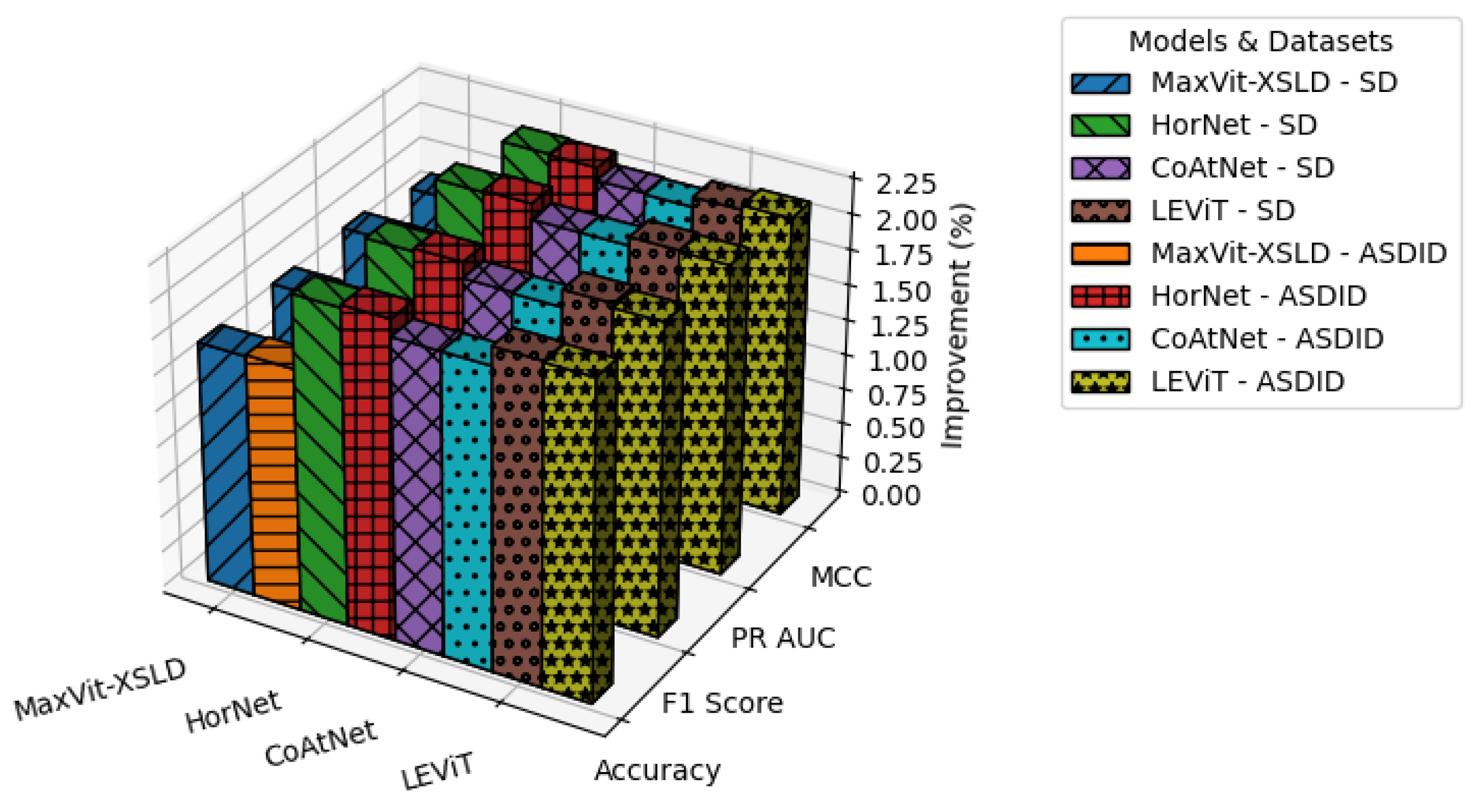
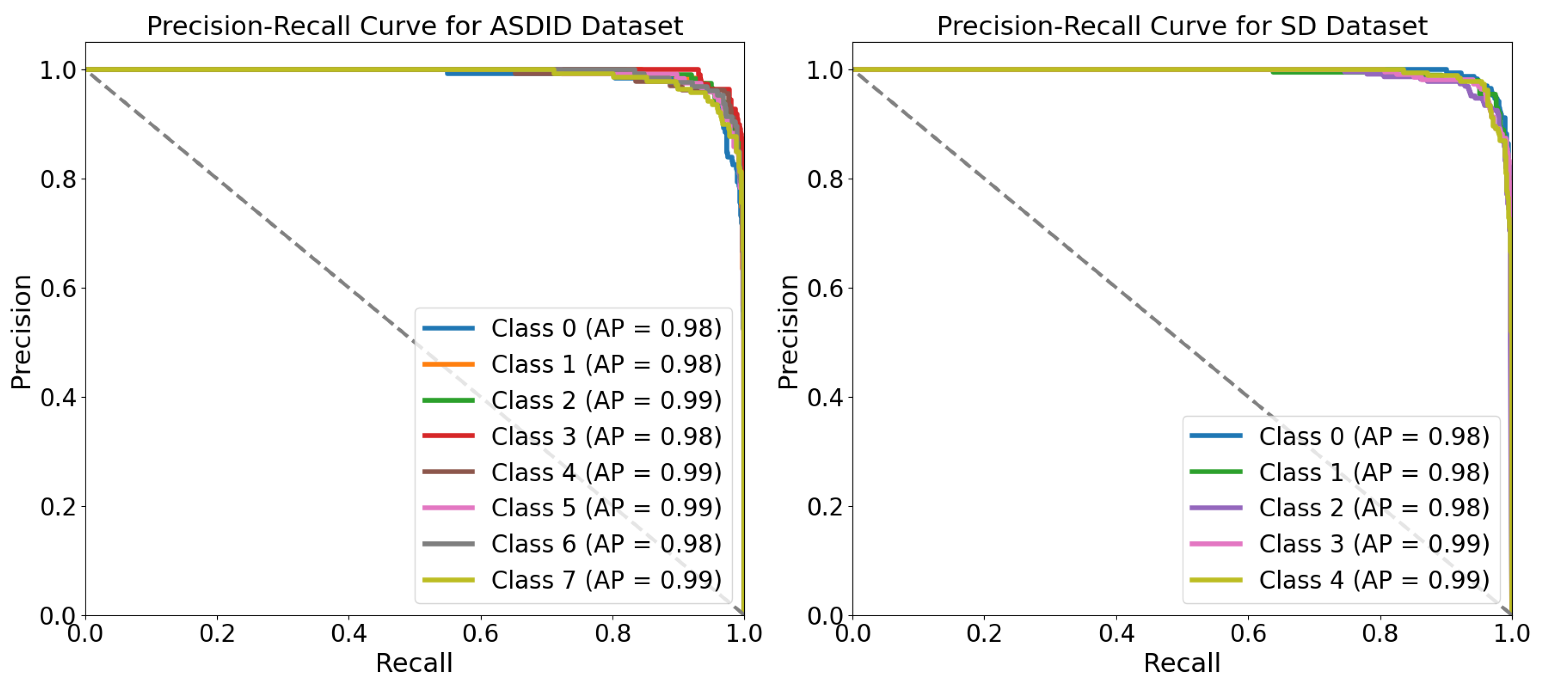
The proposed MaxVit-XSLD method outperforms other models due to its hybrid architecture that merges MBConv layers with multiaxis self-attention mechanisms. The MBConv layers effectively extract local spatial features like lesions and textural anomalies while reducing computational overhead through depthwise separable convolutions and squeeze-and-excitation (SE) blocks. This approach maintains essential spatial relationships with fewer parameters, enhancing efficiency. The multiaxis attention mechanisms capture long-range global dependencies and spatial relationships essential for identifying disease progression patterns, such as pigmentation anomalies. This combination of local and global feature extraction gives MaxVit-XSLD a greater contextual understanding and generalization capability than traditional convolutional networks, which often struggle with long-range dependencies.

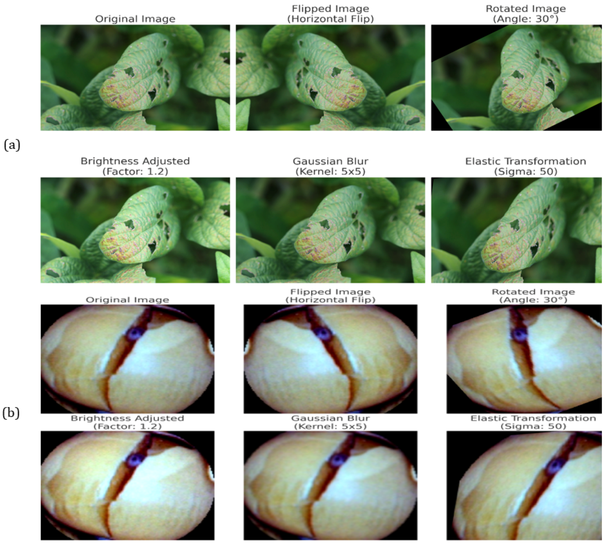
Additionally, the augmentation increases the diversity of the dataset and helps with class imbalances to enhance model performance. To simulate real-world conditions like occlusions and the different conditions of illumination, techniques such as elastic deformations, Gaussian noise injection, and random rotations are used to simulate brightness adjustments. This makes the Seed Disease (SD) dataset more diverse as well as balanced in the class distribution. Therefore, the model has less bias and is more sensitive to the underrepresented classes, and the Average Sensitivity and Diagnostic Inference metrics that it uses are effective in the generalization to unseen data. Standardizing overfits metadata but also guarantees that pretrained weights are compatible with this standard and speeds up convergence during transfer learning. Also, the preprocessing stage mitigates irrelevant variations on the feature space and increases the feature alignment between the images. Augmenting our data and preprocessing are combined to create an input pipeline that robustly allows us to optimally train the model and for it to analyze many complex patterns.

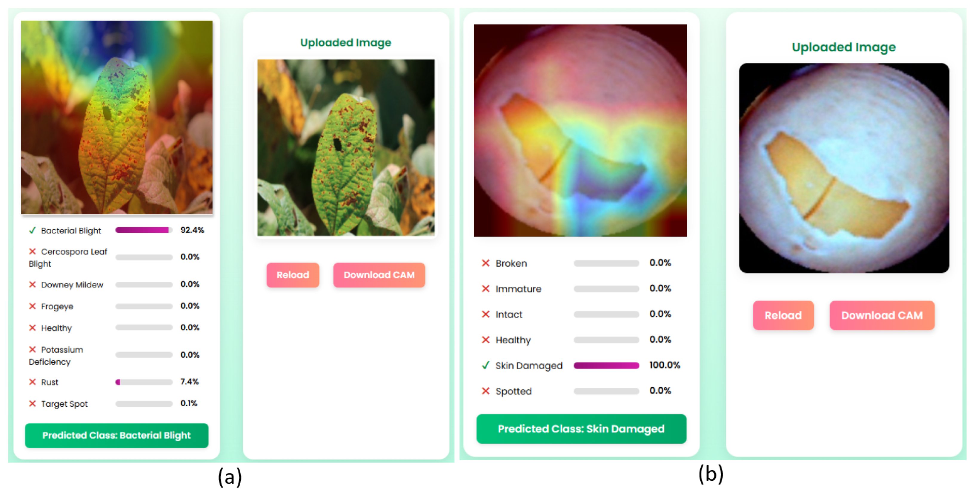
The SoyScan application is designed to improve soybean disease diagnostics by combining high-precision classification using the MaxViT-XSLD architecture with robust interpretability through explainable AI (XAI) methodologies. It utilizes GradCAM to generate class-discriminative localization maps that visually highlight important pathological features, such as necrotic lesions, leaf discoloration, and structural seed anomalies. These visual attributions enhance model interpretability, fostering algorithmic accountability and building user trust among agronomists, researchers, and non-expert stakeholders. SoyScan facilitates rapid detection and decision support, helping to minimize yield loss and economic impact. Its modular micro-service architecture is built for extensibility, allowing for the seamless integration of additional crop models, region-specific disease classifications, and multilingual interfaces, ensuring global adaptability. The system’s design aligns with the principles of trustworthy and human-centric AI, addressing regulatory and user demands for explainability, fairness, and reliability. Moreover, SoyScan is structured for future integration with IoT-enabled sensors and geospatial data streams, paving the way for a scalable and interoperable solution within precision agriculture and smart farming ecosystems.

While GradCAM significantly improves interpretability by visually localizing areas that are critical for class differentiation, it is not without its limitations and challenges. GradCAM relies heavily on the gradient flow from the final convolutional layers, which restricts its resolution and spatial accuracy—especially in Transformer-based architectures like MaxViT-XSLD, where attention mechanisms are more prominent than spatial convolutions. This reliance can produce coarse saliency maps, making it difficult to discern subtle pathological cues such as micro-lesions or fine texture variations in soybean leaf and seed images. In scenarios with high intra-class similarity (e.g., Cercospora leaf blight and frogeye leaf spot), GradCAM may generate overlapping heatmaps, which can reduce class separability and the clarity of interpretation. Furthermore, the technique is sensitive to input variations; minor changes in lighting, occlusions, or image noise can result in unstable gradient attributions, leading to misleading or diffused activation maps. GradCAM also does not include a built-in confidence metric, which means that the saliency visualization may look equally strong for both high-certainty and low-certainty predictions, potentially confusing users. Moreover, in the context of the SD dataset, where morphological differences are subtle (e.g., between immature and intact seeds), the lack of pixel-level detail may limit actionable insights.

Several improvements can be implemented to address these limitations. First, integrating high-resolution attribution methods like Score-CAM, GradCAM++, or Layer-wise Relevance Propagation (LRP) can capture nuanced spatial features that are crucial for distinguishing visually similar classes. Additionally, combining saliency maps from multiple layers—both earlier and deeper—can enhance localization accuracy and contextual relevance. Incorporating uncertainty quantification techniques, such as Monte Carlo Dropout or Deep Ensembles, can help align prediction confidence with the reliability of heatmaps, minimizing the risk of overinterpreting ambiguous outputs. To improve interpretability for non-expert users, the system could feature semantic segmentation overlays alongside GradCAM visualizations, explicitly marking diseased regions. Additionally, creating interactive XAI dashboards with adjustable attention thresholds and class attribution toggles can empower users to explore the reasoning behind decisions dynamically. Finally, training with counterfactual explanations and objectives focused on adversarial robustness can lead to more stable and resilient visual attributions.

SoyScan has several technical and practical limitations in various agricultural environments. The MaxViT-XSLD model relies on combined multiaxis attention with MBConv modules, making it computationally demanding. In this study, it requires 45.2 GFLOPs and over 11 GB of GPU memory, and it consumes approximately 9.8 W of power per inference. These hardware requirements present major challenges for scalability, especially in resource-constrained or embedded edge devices commonly used in rural farming contexts. In contrast, lighter models like LEViT, which require significantly less computational power and offer faster inference times, are more appropriate for mobile or edge deployment scenarios where hardware resources are limited. This trade-off ensures flexibility depending on deployment needs, balancing between predictive power and hardware efficiency. Additionally, MaxViT’s deep and multibranch architecture increases training complexity and sensitivity to hyperparameter settings, which can lead to convergence issues or overfitting when applied to smaller datasets. While MaxViT-XSLD shows strong performance on the ASDID and SD datasets, its adaptability to real-world scenarios may be limited by domain shift. These datasets may not adequately represent the full range of environmental variability, soybean cultivar diversity, or disease phenotypes found in different regions. The model’s Grid and Block Attention mechanisms may struggle to identify irregular or fine-grained features in noisy, occluded, or variably illuminated images, which can reduce the robustness of its inferences. Integrating GradCAM enhances model explainability, but the abstract attention maps in Transformer-based architectures can be hard for non-technical stakeholders like farmers or field technicians to interpret. Finally, the system’s reliance on stable internet for server-based inference restricts its practical deployment in bandwidth-constrained or offline rural environments.

To enhance both user experience and system robustness, the SoyScan web application can undergo several improvements. First, implementing a model compression pipeline—through methods such as pruning, quantization, or knowledge distillation of the MaxViT-XSLD model—can significantly decrease inference latency and reduce computational overhead. This would allow for seamless deployment on resource-constrained edge devices. Additionally, integrating adaptive image preprocessing techniques like histogram equalization, contrast-limited adaptive histogram equalization (CLAHE), and illumination normalization can help mitigate variability caused by environmental noise. This, in turn, will improve feature stability across diverse field conditions. Using hierarchical GradCAM overlays with adjustable saliency thresholds and semantic segmentation for disease localization can provide more precise visual feedback for non-technical stakeholders. Moreover, implementing a multilingual user interface with responsive design and voice-guided navigation via Web Speech APIs can enhance accessibility for users in rural and linguistically diverse areas. The application’s robustness can be further strengthened by introducing an active learning loop that incorporates user-validated labels to periodically retrain the model, encouraging continual learning and adaptation to specific domains. Additionally, adopting a Progressive Web Application (PWA) architecture will enable offline functionality, background synchronization, and caching of inference models using WebAssembly (WASM) or TensorFlow.js, ensuring consistent operation in low-connectivity regions. Finally, incorporating context-aware metadata (geolocation, timestamps, and crop cycle stages) can allow spatiotemporal disease tracking and provide diagnostic recommendations.

Future work should include neural architecture search (NAS) for developing lightweight Transformer variants for edge devices. Additionally, while the augmentation pipeline enhances dataset diversity, it fails to fully capture real-world variability such as occlusion, complex lighting, and overlapping plant structures. To address this, domain adaptation methods like adversarial domain adaptation and semi-supervised learning should be applied. Using GANs for synthetic data generation could further improve robustness to unseen scenarios. The current focus on static RGB images limits the framework’s ability to track disease progression over time. Incorporating multimodal data sources like hyperspectral, thermal, or LiDAR imaging, along with spatio-temporal architectures, would enhance understanding of disease dynamics. GradCAM’s coarse feature attribution may not suffice for complex disease cases; thus, exploring more precise interpretability techniques like Integrated Gradients or SHAP is necessary for better model insights. Finally, developing mobile-friendly implementations with real-time inference capabilities would enhance accessibility, particularly for resource-constrained farming communities.

6. Conclusions

In this study, we tackled the challenge of accurately identifying soybean diseases by integrating both leaf and seed datasets into a single diagnostic pipeline. While we built on existing techniques—such as the MaxViT, targeted augmentation, and GradCAM explainability—we adapted these components specifically for our domain to create a practical, interpretable, and deployment-ready solution. Our proposed MaxViT-XSLD model effectively captures both local lesion textures and global spatial patterns that are essential for distinguishing various disease traits. Additionally, the SoyScan application combines this model with XAI visualizations, which enhance transparency, usability, and trust among agricultural stakeholders. Although our system demonstrates strong classification performance and offers practical value, it has limitations, such as computational complexity and dependence on static RGB images. These factors may affect its performance in low-resource or variable field conditions. Future research should focus on exploring lightweight Transformer architectures, multimodal datasets with diverse environmental conditions, and more advanced interpretability methods to improve transparency. Developing regulatory-compliant XAI frameworks and testing our approach across more crop categories will boost global adoption in agricultural diagnostics and improve food security.

References

1. Modgil, R.; Tanwar, B.; Goyal, A.; Kumar, V. Soybean (Glycine max). In Oilseeds: Health Attributes and Food Applications; Springer: Berlin/Heidelberg, Germany, 2021; pp. 1–46. [Google Scholar]
2. Mathur, R.K.; Sujatha, M.; Bera, S.K.; Rai, P.K.; Babu, B.K.; Suresh, K.; Babu, S.S.; Sharma, M.; Rani, K.; Ajay, B.C.; et al. Oilseeds and Oil Palm. In Trajectory of 75 Years of Indian Agriculture After Independence; Springer: Berlin/Heidelberg, Germany, 2023; pp. 231–264. [Google Scholar]
3. Singh, P.; Tomar, M.; Singh, A.K.; Yadav, V.K.; Saini, R.P.; Swami, S.R.; Mahesha, H.S.; Singh, A.K.; Singh, T. International scenario of oat production and its potential role in sustainable agriculture. In Oat (Avena sativa): Production to Plate; CRC Press: Boca Raton, FL, USA, 2024; pp. 47–68. [Google Scholar]
4. Grassini, P.; Cafaro La Menza, N.; Rattalino Edreira, J.I.; Monzón, J.P.; Tenorio, F.A.; Specht, J.E. Soybean. In Crop Physiology Case Histories for Major Crops; Academic Press: Cambridge, MA, USA, 2021; pp. 282–319. [Google Scholar]
5. Baetsen-Young, A.M.; Swinton, S.M.; Chilvers, M.I. Economic impact of fluopyram-amended seed treatments to reduce soybean yield loss associated with sudden death syndrome. Plant Dis. 2021, 105, 78–86. [Google Scholar] [CrossRef] [PubMed]
6. Bradley, C.A.; Allen, T.W.; Sisson, A.J.; Bergstrom, G.C.; Bissonnette, K.M.; Bond, J.; Byamukama, E.; Chilvers, M.I.; Collins, A.A.; Damicone, J.P.; et al. Soybean yield loss estimates due to diseases in the United States and Ontario, Canada, from 2015 to 2019. Plant Health Prog. 2021, 22, 483–495. [Google Scholar] [CrossRef]
7. Anjna; Sood, M.; Singh, P.K. Hybrid system for detection and classification of plant disease using qualitative texture features analysis. Procedia Comput. Sci. 2020, 167, 1056–1065. [Google Scholar] [CrossRef]
8. Shaikh, T.A.; Rasool, T.; Lone, F.R. Towards leveraging the role of machine learning and artificial intelligence in precision agriculture and smart farming. Comput. Electron. Agric. 2022, 198, 107119. [Google Scholar] [CrossRef]
9. Delfani, P.; Thuraga, V.; Banerjee, B.; Chawade, A. Integrative approaches in modern agriculture: IoT, ML and AI for disease forecasting amidst climate change. Precis. Agric. 2024, 25, 2589–2613. [Google Scholar] [CrossRef]
10. Karunathilake, E.M.B.M.; Le, A.T.; Heo, S.; Chung, Y.S.; Mansoor, S. The path to smart farming: Innovations and opportunities in precision agriculture. Agriculture 2023, 13, 1593. [Google Scholar] [CrossRef]
11. Mohyuddin, G.; Khan, M.A.; Haseeb, A.; Mahpara, S.; Waseem, M.; Saleh, A.M. Evaluation of machine learning approaches for precision farming in smart agriculture system: A comprehensive review. IEEE Access 2024, 12, 60155–60184. [Google Scholar] [CrossRef]
12. Alsulimani, A.; Akhter, N.; Jameela, F.; Ashgar, R.I.; Jawed, A.; Hassani, M.A.; Dar, S.A. The impact of artificial intelligence on microbial diagnosis. Microorganisms 2024, 12, 1051. [Google Scholar] [CrossRef]
13. Tugrul, B.; Elfatimi, E.; Eryigit, R. Convolutional neural networks in detection of plant leaf diseases: A review. Agriculture 2022, 12, 1192. [Google Scholar] [CrossRef]
14. Peng, M.; Liu, Y.; Khan, A.; Ahmed, B.; Sarker, S.K.; Ghadi, Y.Y.; Bhatti, U.A.; Al-Razgan, M.; Ali, Y.A. Crop monitoring using remote sensing land use and land change data: Comparative analysis of deep learning methods using pre-trained CNN models. Big Data Res. 2024, 36, 100448. [Google Scholar] [CrossRef]
15. Mohammed, A.; Kora, R. A comprehensive review on ensemble deep learning: Opportunities and challenges. J. King Saud Univ.-Comput. Inf. Sci. 2023, 35, 757–774. [Google Scholar] [CrossRef]
16. Khan, S.; Naseer, M.; Hayat, M.; Zamir, S.W.; Khan, F.S.; Shah, M. Transformers in vision: A survey. ACM Comput. Surv. 2022, 54, 1–41. [Google Scholar] [CrossRef]
17. Farah, N.; Drack, N.; Dawel, H.; Buettner, R. A deep learning-based approach for the detection of infested soybean leaves. IEEE Access 2023, 11, 99670–99679. [Google Scholar] [CrossRef]
18. Goshika, S.; Meksem, K.; Ahmed, K.R.; Lakhssassi, N. Deep learning model for classifying and evaluating soybean leaf disease damage. Int. J. Mol. Sci. 2023, 25, 106. [Google Scholar] [CrossRef] [PubMed]
19. Bevers, N.; Sikora, E.J.; Hardy, N.B. Soybean disease identification using original field images and transfer learning with convolutional neural networks. Comput. Electron. Agric. 2022, 203, 107449. [Google Scholar] [CrossRef]
20. Yu, M.; Ma, X.; Guan, H. Recognition method of soybean leaf diseases using residual neural network based on transfer learning. Ecol. Inform. 2023, 76, 102096. [Google Scholar] [CrossRef]
21. Yu, M.; Ma, X.; Guan, H.; Zhang, T. A diagnosis model of soybean leaf diseases based on improved residual neural network. Chemom. Intell. Lab. Syst. 2023, 237, 104824. [Google Scholar] [CrossRef]
22. Hang, Y.; Meng, X.; Wu, Q. Application of improved lightweight network and Choquet fuzzy ensemble technology for soybean disease identification. IEEE Access 2024, 12, 25146–25163. [Google Scholar] [CrossRef]
23. Song, H.; Huang, Y.; Han, T.; Xu, S.; Liu, Q. A cell P system with membrane division and dissolution rules for soybean leaf disease recognition. Plant Methods 2025, 21, 39. [Google Scholar] [CrossRef]
24. Pan, R.; Lin, J.; Cai, J.; Zhang, L.; Liu, J.; Wen, X.; Chen, X.; Zhang, X. A two-stage feature aggregation network for multi-category soybean leaf disease identification. J. King Saud Univ. Comput. Inf. Sci. 2023, 35, 101669. [Google Scholar] [CrossRef]
25. Sharma, V.; Tripathi, A.K.; Mittal, H.; Nkenyereye, L. SoyaTrans: A novel transformer model for fine-grained visual classification of soybean leaf disease diagnosis. Expert Syst. Appl. 2025, 260, 125385. [Google Scholar] [CrossRef]
26. Shahzore, U.; Akbar, S.; Shoukat, I.A.; Rehman, A.; Saba, T.; Sikder, T. A vision transformer-based framework for detection and classification of soybean leaf diseases. In Proceedings of the 2025 8th International Conference on Data Science and Machine Learning Applications (CDMA), Manama, Bahrain, 4–5 March 2025; pp. 138–143. [Google Scholar]
27. Wang, X.; Pan, T.; Qu, J.; Sun, Y.; Miao, L.; Zhao, Z.; Li, Y.; Zhang, Z.; Zhao, H.; Hu, Z.; et al. Diagnosis of soybean bacterial blight progress stage based on deep learning in the context of data-deficient. Comput. Electron. Agric. 2023, 212, 108170. [Google Scholar] [CrossRef]
28. Yu, X.; Chen, C.; Gong, Q.; Li, W.; Lu, L. Soybean leaf diseases recognition based on generative adversarial network and transfer learning. Int. J. Comput. Intell. Appl. 2024, 23, 2350030. [Google Scholar] [CrossRef]
29. Wu, Q.; Ma, X.; Liu, H.; Bi, C.; Yu, H.; Liang, M.; Zhang, J.; Li, Q.; Tang, Y.; Ye, G. A classification method for soybean leaf diseases based on an improved ConvNeXt model. Sci. Rep. 2023, 13, 19141. [Google Scholar] [CrossRef] [PubMed]
30. Zhang, B.; Zhao, D. An ensemble learning model for detecting soybean seedling emergence in UAV imagery. Sensors 2023, 23, 6662. [Google Scholar] [CrossRef] [PubMed]
31. Sable, A.; Singh, P.; Kaur, A.; Driss, M.; Boulila, W. Quantifying soybean defects: A computational approach to seed classification using deep learning techniques. Agronomy 2024, 14, 1098. [Google Scholar] [CrossRef]
32. Zhang, L.; Sun, L.; Jin, X.; Zhao, X.; Li, S. DAFFnet: Seed classification of soybean variety based on dual attention feature fusion networks. Crop J. 2025, 13, 619–629. [Google Scholar] [CrossRef]
33. Yang, X.; Ma, K.; Zhang, D.; Song, S.; An, X. Classification of soybean seeds based on RGB reconstruction of hyperspectral images. PLoS ONE 2024, 19, e0307329. [Google Scholar] [CrossRef]
34. Dioses, I.A.M.; Dioses, J.L.; Aquino, R.N.; Feliciano, C.G.M.; Tababa, J.B.; Hermosura, L.F. Soybean seed quality assessment classification using EfficientNet B0 algorithm. In Proceedings of the 2025 21st IEEE International Colloquium on Signal Processing & Its Applications (CSPA), Penang, Malaysia, 7–8 March 2025; pp. 144–149. [Google Scholar]
35. Lin, W.; Shu, L.; Zhong, W.; Lu, W.; Ma, D.; Meng, Y. Online classification of soybean seeds based on deep learning. Eng. Appl. Artif. Intell. 2023, 123, 106434. [Google Scholar] [CrossRef]
36. Miranda, M.C.D.C.; Aono, A.H.; Pinheiro, J.B. A novel image-based approach for soybean seed phenotyping using machine learning techniques. Crop Sci. 2023, 63, 2665–2684. [Google Scholar] [CrossRef]
37. Chen, X.; He, W.; Ye, Z.; Gai, J.; Lu, W.; Xing, G. Soybean seed pest damage detection method based on spatial frequency domain imaging combined with RL-SVM. Plant Methods 2024, 20, 130. [Google Scholar] [CrossRef] [PubMed]
38. Kaler, N.; Bhatia, V.; Mishra, A.K. Deep learning-based robust analysis of laser bio-speckle data for detection of fungal-infected soybean seeds. IEEE Access 2023, 11, 89331–89348. [Google Scholar] [CrossRef]
39. Lin, W.; Fu, Y.; Xu, P.; Liu, S.; Ma, D.; Jiang, Z.; Zang, S.; Yao, H.; Su, Q. Soybean image dataset for classification. Data Brief 2023, 48, 109300. [Google Scholar] [CrossRef] [PubMed]
40. GB 1352-2009; Soybean. Standardization Administration of China (SAC). China Standards Press: Beijing, China, 2009.
41. Dharani Devi, G.; Jeyalakshmi, J. Privacy-preserving breast cancer classification: A federated transfer learning approach. J. Imaging Inform. Med. 2024, 37, 1488–1504. [Google Scholar]
42. Wu, J.; Guo, Y.; Deng, C.; Zhang, A.; Qiao, H.; Lu, Z.; Xie, J.; Fang, L.; Dai, Q. An integrated imaging sensor for aberration-corrected 3D photography. Nature 2022, 612, 62–71. [Google Scholar] [CrossRef]
43. Shorten, C.; Khoshgoftaar, T.M. A survey on image data augmentation for deep learning. J. Big Data 2019, 6, 1–48. [Google Scholar] [CrossRef]
44. Zheng, S.; Song, Y.; Leung, T.; Goodfellow, I. Improving the robustness of deep neural networks via stability training. In Proceedings of the IEEE Conference on Computer Vision and Pattern Recognition (CVPR), Las Vegas, NV, USA, 27–30 June 2016; pp. 4480–4488. [Google Scholar]
45. Grigoras, C.C.; Zichil, V.; Ciubotariu, V.A.; Cosa, S.M. Machine learning, mechatronics, and stretch forming: A history of innovation in manufacturing engineering. Machines 2024, 12, 180. [Google Scholar] [CrossRef]
46. Simard, P.Y.; Steinkraus, D.; Platt, J.C. Best practices for convolutional neural networks applied to visual document analysis. In Proceedings of the ICDAR, Edinburgh, Scotland, 3–6 August 2003; Volume 3. [Google Scholar]
47. Queiroz Nogueira Lira, R.; Motta de Sousa, L.G.; Memoria Pinho, M.L.; Pinto da Silva Andrade de Lima, R.C.; Garcia Freitas, P.; Scholles Soares Dias, B.; Breda de Souza, A.C.; Ferreira Leite, A. Deep learning-based human gunshot wounds classification. Int. J. Leg. Med. 2025, 139, 651–666. [Google Scholar] [CrossRef]
48. Prabowo, D.P.; Rohman, M.S.; Megantara, R.A.; Pergiwati, D.; Saraswati, G.W.; Pramunendar, R.A.; Shidik, G.F.; Andono, P.N. Adaptive Inertia Weight Particle Swarm Optimization for Augmentation Selection in Coral Reef Classification with Convolutional Neural Networks. JOIV Int. J. Inform. Vis. 2025, 9, 216–223. [Google Scholar] [CrossRef]
49. Kalaivani, S.; Asha, N.; Gayathri, A. Geometric transformations-based medical image augmentation. In GANs for Data Augmentation in Healthcare; Springer: Berlin/Heidelberg, Germany, 2023; pp. 133–141. [Google Scholar]
50. Graham, B.; El-Nouby, A.; Touvron, H.; Stock, P.; Joulin, A.; Jégou, H.; Douze, M. LeViT: A Vision Transformer in ConvNet’s Clothing for Faster Inference. In Proceedings of the IEEE/CVF International Conference on Computer Vision (ICCV), Montreal, QC, Canada, 11–17 October 2021; pp. 12259–12269. [Google Scholar]
51. Liu, P.; Han, S.; Rong, N. Frequency stability prediction of renewable energy penetrated power systems using CoAtNet and SHAP values. Eng. Appl. Artif. Intell. 2023, 123, 106403. [Google Scholar] [CrossRef]
52. Polly, R.; Devi, E.A. Semantic segmentation for plant leaf disease classification and damage detection: A deep learning approach. Smart Agric. Technol. 2024, 9, 100526. [Google Scholar] [CrossRef]
53. Rao, Y.; Zhao, W.; Tang, Y.; Zhou, J.; Lim, S.N.; Lu, J. HorNet: Efficient high-order spatial interactions with recursive gated convolutions. Adv. Neural Inf. Process. Syst. 2022, 35, 10353–10366. Available online: https://github.com/raoyongming/HorNet (accessed on 26 January 2025).
54. Yang, L.; Mohamed, A.S.A.; Ali, M.K.M. Traffic conflicts analysis in Penang based on improved object detection with transformer model. IEEE Access 2023, 11, 84061–84073. [Google Scholar] [CrossRef]
55. Pacal, I. Enhancing crop productivity and sustainability through disease identification in maize leaves: Exploiting a large dataset with an advanced vision transformer model. Expert Syst. Appl. 2024, 238, 122099. [Google Scholar] [CrossRef]
56. Tu, Z.; Talebi, H.; Zhang, H.; Yang, F.; Milanfar, P.; Bovik, A.; Li, Y. MaxViT: Multi-axis vision transformer. In Proceedings of the European Conference on Computer Vision (ECCV), Tel Aviv, Israel, 23–27 October 2022; pp. 459–479. [Google Scholar]
57. Gorodkin, J. Comparing two K-category assignments by a K-category correlation coefficient. Comput. Biol. Chem. 2004, 28, 367–374. [Google Scholar] [CrossRef]
Figure 1. Overview of the proposed methodology for soybean leaf and seed disease classification. The workflow includes dataset details (ASDID and SD), preprocessing techniques (resizing, normalization, flipping, rotation, brightness adjustment, elastic transformations, and Gaussian noise), evaluation metrics (micro-accuracy, micro-F1, MCC, micro-PR-AUC, learning curves, and confusion matrices), ViT models, and an XAI-integrated web application (SoyScan) with GradCAM visualizations for transparent diagnostics.
Computers 14 00197 g001
Figure 2. Representative images illustrating disease and health categories from the two datasets: (a) soybean leaf disease classes in the ASDID dataset, including bacterial blight, Cercospora leaf blight, downy mildew, healthy, target spot, soybean rust, potassium deficiency, and frogeye; (b) soybean seed defect classes in the SD dataset, comprising broken, immature, intact, skin-damaged, and spotted.
Computers 14 00197 g002
Figure 3. Sample output images from the preprocessing pipeline applied to (a) the ASDID and (b) the SD datasets. The preprocessing techniques include horizontal flipping, rotation (30°), brightness adjustment (factor: 1.2), Gaussian blur (kernel: 5 × 5), and elastic transformations (sigma: 50).
Computers 14 00197 g003
Figure 4. LEViT model architecture.
Computers 14 00197 g004
Figure 5. CoAtNet architecture.
Computers 14 00197 g005
Figure 6. Hornet architecture. The symbol * denotes spatial dimensions of the feature maps, which vary depending on the input resolution.
Computers 14 00197 g006
Figure 7. Adapted from the original MaxViT architecture by Tu et al. [56], the proposed MaxViT-XSLD integrates the core multiaxis attention and MBConv blocks for dual-domain soybean disease diagnostics. It starts with a stem block of two 3 × 3 convolutions, downsampling the input (224 × 224) to 112 × 112. This is followed by stacked MaxViT blocks (S1–S4) with decreasing resolutions (56 × 56 to 7 × 7), each comprising MBConv for feature extraction, Block Attention (Block-SA) for local context, and Grid-SA for global dependencies. The model concludes with pooling, a fully connected layer, and an output head.
Computers 14 00197 g007
Figure 8. Comparison of model performance before and after data augmentation on SD and ASDID datasets.
Computers 14 00197 g008
Figure 9. Percentage improvements of TL models on SD and ASDID datasets.
Computers 14 00197 g009
Figure 10. Computational trade-offs radar chart.
Computers 14 00197 g010
Figure 11. Statistical significance (p-values) of MaxViT-XSLD compared to HorNet, CoAtNet, and LEViT.
Computers 14 00197 g011
Figure 12. Confusion matrices illustrating classification performance for (a) soybean leaf diseases using the ASDID dataset and (b) soybean seed conditions using the SD dataset.
Computers 14 00197 g012
Figure 13. Learning curves for (a) soybean leaf diseases using the ASDID dataset and (b) soybean seed conditions using the SD dataset.
Computers 14 00197 g013
Figure 14. ROC AUC curves of the proposed model on ASDID and SD datasets.
Computers 14 00197 g014
Figure 15. Precision–recall curves of the proposed model on ASDID and SD datasets.
Computers 14 00197 g015
Figure 16. GradCAM visualizations show key areas for model predictions in (a) soybean leaf diseases (ASDID dataset) and (b) soybean seed defects (SD dataset). These outputs reveal that the proposed method emphasizes crucial biological features, including diseased leaf regions and seed defects.
Computers 14 00197 g016
Figure 17. The SoyScan web application showcases interpretable classification of soybean diseases utilizing GradCAM visualizations. It includes (a) a predicted bacterial blight classification for a soybean leaf sample from the ASDID dataset and (b) a predicted skin damage classification for a soybean seed sample from the SD dataset. The highlighted regions in the visualizations support these predictions.
Computers 14 00197 g017