Simulation Application of Adaptive Strategy Hybrid Secretary Bird Optimization Algorithm in Multi-UAV 3D Path Planning

Abstract

Multi-UAV three-dimensional (3D) path planning is formulated as a high-dimensional multi-constraint optimization problem involving costs such as path length, flight altitude, avoidance cost, and smoothness. To address this challenge, we propose an Adaptive Strategy Hybrid Secretary Bird Optimization Algorithm (ASHSBOA), an enhanced variant of the Secretary Bird Optimization Algorithm (SBOA). ASHSBOA integrates a weighted multi-direction dynamic learning strategy, an adaptive strategy-selection mechanism, and a hybrid elite-guided boundary-repair scheme to enhance the ability to identify local optima and balance exploration and exploitation. The algorithm is tested on benchmark suites CEC-2017 and CEC-2022 against nine classic or state-of-the-art optimizers. Non-parametric tests show that ASHSBOA consistently achieves superior performance and ranks first among competitors. Finally, we applied ASHSBOA to a multi-UAV 3D path planning model. In Scenario 1, the path cost planned by ASHSBOA decreased by 124.9 compared to the second-ranked QHSBOA. In the more complex Scenario 2, this figure reached 1137.9. Simulation results demonstrate that ASHSBOA produces lower-cost flight paths and more stable convergence behavior compared to comparative methods. These results validate the robustness and practicality of ASHSBOA in UAV path planning.

1. Introduction

Unmanned aerial vehicles (UAVs) are a type of aerial bionic robot. Initially, UAVs were exclusively used for military applications and were experimented with during World War II [1]. Recently, the use of UAVs for transportation and logistics has attracted widespread attention. Especially after the outbreak of COVID-19, the possibility of contactless delivery has led to a surge in interest in UAV-based logistics [2]. This has further contributed to the growing popularity of UAV mission planning problems, including UAV last-mile package delivery [3], in the context of the “low-altitude economy.” Within the field of robot mission planning, UAV path planning is recognized as a high-dimensional optimization problem [4,5]. Over time, UAV systems have become more and more autonomous, and their performance and efficacy have also become more advanced [6] and have been widely applied in fields such as tracking [7], meteorology [8], monitoring [9], rescue search [10], surveillance [11], and agriculture support [12].

For UAVs, good or bad path planning is directly related to the efficiency and safety of them [13]. Among them, multi-UAV operation is a more complex and time-consuming research topic, with higher computational costs compared to single-UAV missions [14]. At the same time, the efficiency of path planning is a fundamental element of UAV planning. It helps UAVs calculate the best route from their current spot to the destination, and they also avoid obstacles and stick to operational limits [15]. Global path planning and small-scale path planning are two important components of UAV autonomous flight [16].

In static environments where terrain and obstacles are predetermined, a series of well-recognized algorithms have been developed for global path planning of UAVs. These include two classic graph search algorithms, namely the A* algorithm [17] and Dijkstra’s algorithm [18], as well as genetic algorithms (GAs) [19], particle swarm optimization (PSO) [20], differential evolution (DE) [21], and ant colony optimization (ACO) [22]. Thanks to their unique advantages in terms of fitness and computational efficiency, these algorithms have become important tools in the field of UAV path planning and other engineering application domains.

Extensive improvements have been made based on the above classic algorithms to promote their behavior. Geng et al. [23] proposed an A* to solving multi-UAV path planning problems and evaluated its effectiveness in two types of 3D environments: one with cubic obstacles and mountains, and the other with only mountains. The experimental results showed that compared with other path planning methods, this A* algorithm could provide the optimal path, but with a slightly longer computation time. Bai et al. [24] proposed a hybrid method combining the A* algorithm and the dynamic window approach (DWA) for UAV path planning. Tianzhu et al. [25] put forward an improved A* algorithm for optimizing UAV 3D path planning and evaluated the algorithm’s performance through three different experiments. The simulation results indicated that the improved A* algorithm performed better in terms of cost-effectiveness and path length optimization. A bidirectional adaptive A* algorithm for UAV path planning problems was proposed by Wu et al. [26]. Chen et al. [27] proposed improvements to the traditional A* algorithm for static environments to overcome its limitations. In addition, there is a fusion way that joins the improved A* algorithm with quadratic programming. It works well for UAV trajectories in messy and complex airspaces [28]. This method may encounter obstacles in terms of the availability of computing resources. To extend the A* algorithm, De Filippis et al. [29] developed a new heuristic method called the Theta* algorithm. Compared with the A* algorithm, experiments have proven the superiority of the Theta* algorithm in path cost optimization and constraint handling. For the Dijkstra, Maini and Sujit [30] invented a new method based on the Dijkstra algorithm that considers turning angle restrictions. The experimental results showed that this method was superior to the traditional Dijkstra algorithm in path length and collision avoidance performance.

In terms of classical metaheuristic algorithms, Guangxing et al. [31] improved the traditional ant colony optimization (ACO) algorithm by refining the pheromone rules and adjusting the weighting factors. Liu et al. modified the traditional ACO algorithm by incorporating an elite ant pheromone update system, aiming to achieve higher convergence accuracy with fewer iterations [32]. Song et al. combined multiple heuristic elements and imposed restrictions on pheromone levels to prevent the ACO algorithm from reaching local optimal conditions [33]. Zhang et al. [34] drew an improved DE algorithm specifically designed to optimize UAV trajectory planning in mountainous terrain. Chen et al. developed an algorithm named ACVDEPSO, which includes new parameters such as cylindrical vectors and different evolution operators [35]. This algorithm combines cylindrical coordinates and an adaptive parameter strategy with differential evolution to improve path planning in complex 3D scenarios. Yu et al. [36] proposed a method that combines the Grey Wolf Optimizer (GWO) with the DE algorithm to improve UAV path planning; however, mixed algorithms generally increase the complexity of the algorithm. Zhang et al. [37] put forward another hybrid algorithm (HDEFWA), which combines DE and the Fireworks Algorithm (FWA) to optimize UAV path planning. For PSO algorithm, Mingyu et al. introduced an improved PSO method based on time-varying adaptive inertia weights for 2D settings with static obstacles [38]. In addition, Manh et al. [13] created a spherical vector-based particle swarm optimization (SPSO) method, which uses spherical vectors to represent the motion state of unmanned aerial vehicles to optimize path planning. For the Genetic Algorithm (GA), Majeed et al. proposed a GA-based method [39]. Although this method effectively addresses many objectives and constraints, it encounters difficulties in terms of scalability. Shivgan et al. used GA in their research to reduce the energy consumption of UAV flights [40]. To improve the efficiency, Arantes et al. studied how heuristic methods and genetic algorithms can work synergistically [41]. Galvez et al. found that using a hybrid method increases the probability of convergence to a local optimum solution. The efficiency of genetic algorithms in three-dimensional path planning has been verified in terms of avoiding radar coverage areas [42].

Small-scale path planning is employed to handle dynamic situations, requiring UAVs to adjust their directions in real-time in response to unexpected events. Its strategies prioritize rapid decision-making and computational efficiency, but often struggle to find optimal solutions. In this situation, rapid exploration random trees (RRT) emerged as a sample-based method [43]. Yang et al. [44] developed a Gaussian process-based RRT (GP-RRT), which integrates a Gaussian process (GP) map construction model into the RRT algorithm to solve UAV path planning problems. Meng et al. [45] drew a new method for path planning of UAVs based on RRT. The results indicated that the improved RRT algorithm can ensure safe and collision-free paths within a wider range. Artificial potential field (APF) uses gravity and repulsive forces to enable drones to move toward their destination while avoiding obstacles. Regarding its improved versions, Moon et al. [46] proposed a hybrid method combining APF and A*, aiming to solve the multi-UAV path planning problem in a 3D dynamic environment. Verified by three fixed-wing UAVs, the results showed that UAVs can plan optimal paths without collisions. Hao et al. [47] improved the APF algorithm by fusing attraction and repulsion to tease out local optima. In addition, other small scale path planning algorithms include fuzzy logic (FL) [48], neural networks (NN) [49], and reinforcement learning (RL) [50].

Global optimization methods have become more prevalent in their path planning, as they can handle various UAV constraints and find global optima in complex scenarios. A large number of metaheuristic algorithms and their improved versions have been developed so far, such as some highly cited and novel algorithms: Harris Hawks Optimization (HHO, 2019) [51], Grey Wolf Optimizer (GWO, 2014) [52], Black-winged Kite Algorithm (BKA, 2024) [53], Crested Porcupine Optimizer (CPO, 2024) [54], Dung Beetle Optimizer (DBO, 2022) [55], Polar Lights Optimizer (PLO, 2024) [56], Whale Optimization Algorithm (WOA, 2016) [57], etc. These methods simulate biological processes. In these processes, solutions are viewed as individuals—they produce new candidate solutions through reproduction and mutation, which may be better suited to specific problems [58]. They are used to solve problems such as path optimization, collaborative planning, and dynamic design of multi-UAV platforms [16]. In order to solve the issues, this study proposes a multi-strategy improved SBOA based on the standard SBOA for 3D path planning of UAVs in complex terrains. The algorithm promotes the behavior of the original algorithm by introducing three major improvement strategies. The main contents of this study are introduced step by step as follows:

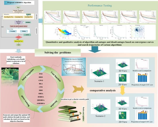
• A novel Adaptive Strategy Hybrid Secretary Bird Optimization Algorithm (ASHSBOA) is proposed, which integrates three innovative improvement strategies into the original Secretary Bird Optimization Algorithm (SBOA). This enhancement aims to boost the algorithm’s capability in solving practical application problems.
• The ASHSBOA is subjected to multi-angle and multi-time tests on two sets of benchmark functions, namely CEC2017 and CEC2022, to evaluate its performance both quantitatively and qualitatively. Additionally, the Wilcoxon test and the Friedman test are serviced to assess the statistically significant differences between the ASHSBOA and the others.
• A multi-UAV path planning model is constructed to test the performance of ASHSBOA in real-world application issues.

The outline of the other parts of this manuscript is as follows. Section 2 introduces the proposal and related developments of the original SBOA. Section 3 notes on the design background and principles of the standard SBOA, along with a description of the multi-UAV path planning model. Section 4 explains and analyzes the strategies of the improved algorithm and its complexity. Section 5 presents the benchmark function tests and statistical tests for algorithms. Section 6 conducts experimental simulations and result analysis. Finally, Section 7 draws conclusions and future works.

2. Related Work

The proposal of the Secretary Bird Optimization Algorithm (SBOA) has provided new insights for numerous global optimization problems, including engineering applications and UAV path planning. This algorithm was first proposed by Fu et al. in 2024 [59]. SBOA mimics the survival behaviors of secretary birds in nature, taking their hunting behaviors as a model. It shapes the algorithm’s optimization strategies in the exploration and exploitation phases through two aspects—preying and avoiding natural enemies—and it iteratively repeats these two phases to find the best solution to the problem. Specifically, the exploration phase is divided into three time periods according to the number of iterations: searching, consuming, and attacking for prey. The exploitation phase is further divided into two modes: camouflage when encountering enemies and rapid escape. In the research by Fu et al., SBOA was tested against 15 advanced algorithms on the CEC2017 and CEC2022 benchmark suites to verify its performance. In addition, SBOA has been used in 12 engineering applications and UAV 3D path planning. The conclusion has demonstrated the promising prospects of this algorithm in solving practical optimization problems.

Although the SBOA has been recognized for its adaptability and robustness since its introduction, issues such as convergence and parameter sensitivity still exist [60]. This is because the 3D UAV path planning problem is nonlinear, high-dimensional, and subject to multiple constraints. For this reason, scholars have conducted research on the original SBOA, aiming to address its limitations and improve its robustness. Lyu et al. [61] introduced an Augmented Gold Rush Optimizer with SBOA (AGRO-SBOA), which incorporates several enhancement features: first, improving global exploration and accelerating convergence through well-point set population initialization; second, enhancing exploration performance and population diversity with dynamic Lévy flight search; third, updating individuals using dynamic centroid opposition-based learning technology to improve population quality and accuracy; fourth, further refining the exploration–exploitation balance to enhance convergence efficiency and prevent stagnation in local optima; and finally, ensuring greater population diversity through dynamic tangent flight to avoid premature convergence. Jia et al. [62] introduced ACOA-SBOA, which is the Adaptive Coati Optimization Algorithm mixed with Secretary Bird Optimization. It integrates strategies such as chaotic mapping, random proton dynamic antagonistic learning, and adaptive Lévy flight. The algorithm was evaluated in terms of population diversity and convergence behavior. Results from the benchmark functions and Wilcoxon test showed that its performance is superior to that of COA and other advanced optimization technologies. Its reliability in dealing with complex optimization tasks was further proven by using it in five real engineering problems and complex 3D UAV path planning situations.

Additionally, in order to address discrete optimization problems, the Discrete Secretary Bird Optimization Algorithm (D-SBOA) [63] was proposed for routing optimization in wireless sensor networks (WSNs). For solving practical engineering problems, Maurya et al. [64] put forward the Hybrid Secretary Bird Optimization (HSBO) algorithm, which enhances the original SBO through Cauchy mutation and opposition-based learning. The algorithm minimizes power loss and voltage deviation for different load models in 85-node, 141-node, and 415-node optimized radial distribution system test systems. Compared with other methods, it exhibits excellent performance, significantly reducing technical losses and economic costs. Zhu et al. [65] drew a better Secretary Bird Optimization Algorithm (QHSBOA) for chronic disease classification problems and constructed a QHSBOA-KELM diabetes classification model combined with Kernel Extreme Learning Machine (KELM), providing a new approach for early diagnosis of diabetes.

3. Preliminary

3.1. Secretary Bird Optimization Algorithm

The Secretary Bird Optimization Algorithm (SBOA) is a population-based stochastic heuristic optimization method that simulates the wild behaviors of African “secretary birds” in their natural habitat (as shown in Figure 1). It performs exploration and exploitation in the search space through behaviors of hunting and escape from natural enemies:

Exploration: simulates the secretary birds’ strategies for hunting snakes (searching, exhausting, attacking prey). Exploitation: mimics the secretary birds’ strategies for evading natural enemies (environmental camouflage or rapid escape).

The algorithm proceeds iteratively, where the position of each individual corresponds to a candidate solution. Each iteration consists of alternating updates between the “predation” phase and “escape (exploitation)” phase until the termination condition is met.

3.1.1. Initialization

Like most population-based metaheuristic algorithms, SBOA generates N individuals within the search space through random initialization, where each individual represents the position of a secretary bird in the D-dimensional search space.

$$x_{i,j}=l{b}_j+r\times (u{b}_j-l{b}_j),\hspace{1em}r ~ U(0,1)$$

(1)

where the individual’s location i in the j-th dimension is denoted as $x_{i,j}$ and $l{b}_j, u{b}_j$ is the variable boundary. The fitness vector of each individual is calculated in every generation $F={[F(x_1),\dots ,F(x_N)]}^{\top }$.

3.1.2. Exploration Phase (Hunting Strategy)

The predation process is divided into three time periods: $t<{\displaystyle \frac{1}{3}}T$ (searching for prey), ${\displaystyle \frac{1}{3}}T<t<{\displaystyle \frac{2}{3}}T$ (consuming prey), and ${\displaystyle \frac{2}{3}}T<t<T$ (attacking prey), where t represents the current iteration position and T is the maximum iteration number. Different update strategies are used in each stage to enhance global/local search capabilities. In the prey search stage, an idea similar to differential evolution (Equation (2)) is used to enhance global search capabilities.

$$X_{ij}^{\mathrm{new}}=x_{ij}+(x_{\mathrm{random}1}-x_{\mathrm{random}2})\times R_1$$

(2)

where R₁ is a random variable between $[0,1]$, and the update condition is greedy selection (only the optimal solution is retained).

$$X_i=\left\{\begin{array}{l}{X}_i^{new},if F_i^{new}<F_i\hfill \\ X_i,else\hfill \end{array}\right.$$

(3)

where $X_i^{new}$ denotes the new location of the i-th individual in the first stage. $X_{ij}^{\mathrm{new}}$ denotes the value of its j-th dimension. $x_{\mathrm{random}1}$ and $x_{\mathrm{random}2}$ are the random candidate solutions in the first stage.

During the prey consumption phase, Brownian motion is introduced as an intermediate disturbance source and a term that approaches the historical optimum, in order to achieve a transition from coarse to fine. The Brownian disturbance vector is defined as Equation (4):

$$RB=randn(1,Dim)$$

(4)

When in intermediate stage ${\displaystyle \frac{1}{3}}T<t<{\displaystyle \frac{2}{3}}T$, the position is updated using Equation (5):

$$x_{i,j}^{new}=x_{best,j}+\exp \left({(t/T)}^4\right)\cdot (R{B}_j-0.5)\cdot \left(x_{best,j}-x_{i,j}\right)$$

(5)

$$X_i=\left\{\begin{array}{c}{x}_i^{\mathrm{new}}, \mathrm{if} F(x_i^{\mathrm{new}})<F(x_i),\hfill \\ x_i,\hspace{1em} \mathrm{otherwise}.\hfill \end{array}\right.$$

(6)

If the new solution is better adapted, then the original individual is replaced with Equation (6). The exponential term $\exp ({(t/T)}^4)$ searches the search range adaptively with iterations. In the attacking prey phase, the algorithm introduces Lévy flight as a long jump mechanism at a later stage to prevent falling into suboptimal values, and the position is updated to Equation (7):

$$x_{i,j}^{new}=x_{best,j}+\left({\left(1-t/T\right)}^{(2\times t/T)}\right)\times x_{i,j}\times RL$$

(7)

If the new solution is better, then the greedy replacement strategy is still used, where $RL=0.5\times Levy\left(Dim\right)$ is the weighted Lévy step size, calculated as Equation (8):

$$Levy(D)=s\times {\displaystyle \frac{u}{|v{|}^{1/b}}},\hspace{1em}u ~ N(0,s^2), v ~ N(0,1)$$

(8)

where the Lévy distribution is calculated using standard parameters (s = 0.01, λ = 1.5) to achieve a mixed search mechanism of ‘short steps + occasional long jumps’. The standard expression for σ is given by Equation (9):

$$\sigma ={\left({\displaystyle \frac{\mathrm{\Gamma }(1+\beta )\sin (\pi \beta /2)}{\mathrm{\Gamma }(\frac{1+\beta }{2}) \beta 2^{(\beta -1)/2}}}\right)}^{1/\beta }$$

(9)

3.1.3. Exploitation Phase (Escape Strategy)

When the secretary bird encounters a predator, it employs various escape strategies to protect itself. When the algorithm simulates ‘escape from predators,’ two mutually exclusive strategies are introduced: environmental camouflage C1 and rapid escape C2. Let $r=0.5$, a random normal vector $R_2=\mathrm{randn}(1,Dim)$, a candidate solution selected randomly out of the current population or search domain $x_{\mathrm{random}}$, and an integer constant $K=\mathrm{round}(1+\mathrm{rand}(1,1))\in \{1,2\}$.

If it falls into the C1 (disguise) situation, the individual moves to the current global optimal position and combines a random proportion RB with an iterative decay factor:

$$x_{i,j}^{\mathrm{new}}=x_{\mathrm{best},j}+(2\times RB-1)\times {(1-t/T)}^2\times x_{i,j}.$$

(10)

If the situation falls into C2 (escape), use random candidate solution $x_{\mathrm{random}}$ and shaping constant K ∈ {1,2} to perform perturbation:

$$x_{i,j}^{\mathrm{new}}=x_{i,j}+R_{2,j}\times (x_{\mathrm{random},j}-K\cdot x_{i,j}).$$

(11)

The combined formula can be expressed as

$$x_{i,j}^{new}=\left\{\begin{array}{ll}{x}_{best,j}+(2R{B}_j-1) {(1-t/T)}^2{x}_{i,j},\hfill & if (choose C1),\hfill \\ x_{i,j}+R_{2,j} (x_{random,j}-K{x}_{i,j}),\hfill & otherwise (C2).\hfill \end{array}\right.$$

(12)

$$X_i=\left\{\begin{array}{l}{x}_i^{new}, if F(x_i^{new})<F(x_i),\hfill \\ x_i,\hspace{1em} otherwise.\hfill \end{array}\right.$$

(13)

The same greedy strategy is used to update the position. This design balances early exploration and late exploitation through a perturbation factor ${(1-t/T)}^2$ that decays with each iteration. It is worth noting that, regardless of the stage, the fitness $F(x_i^{\mathrm{new}})$ of each generated $x_i^{\mathrm{new}}$ is calculated. If $F(x_i^{\mathrm{new}})$ is better than the current $F(x_i)$, the new solution replaces the current solution and the global optimum $x_{\mathrm{best}}$ is updated.

3.2. Multi-UAV Path Planning Model

Within this study, the path planning problem is modeled as a multi-constrained objective optimization problem. The ultimate goal of the function is to minimize flight costs; this total cost consists of four key weighted components: path length cost, threat avoidance cost, altitude cost, and smoothness cost. Let the planned path consist of N discrete waypoints, with waypoint coordinates $P_i=(x_i,y_i,z_i)$, $i=1,2,\dots ,N$. The first waypoint is the starting point, and the last waypoint is the endpoint. When considering terrain effects, the absolute height of the waypoints is represented as $z_i^{abs}=z_i+H(y_i,x_i)$, where H is the terrain elevation data.

3.2.1. Path Length Cost

The path length is the sum of the distances between all path points. In fact, the path ensures continuity for as long as possible by avoiding obstacles, reflecting the time or energy consumption required for flight. It is defined by Equation (14):

$$J_1={\displaystyle \sum _{i=1}^{N-1}‖P_{i+1}^{abs}-P_i^{abs}‖}$$

(14)

where $P_i^{abs}=(x_i,y_i,z_i^{abs})$. Shorter paths usually imply higher task efficiency and lower energy consumption, so there is a tendency to minimize this metric in optimization.

3.2.2. Threat and Obstacle Avoidance Costs

Obstacles are defined as any object that interrupts the path of the UAV. Obstacles can be buildings, mountains, trees, etc. Radars or missiles are considered real threats. A threat cost function is introduced for this. It is assumed that there are M threat zones in the environment, each threat is centered at $(x_k^t,y_k^t,z_k^t)$, and the threat radius is $r_k$. This partial cost is divided into two categories: cylindrical threats and spherical threats, as in Figure 2.

Cylindrical threat:

$$d_{k,i}=Dist((x_k^t,y_k^t),(x_i,y_i),(x_{i+1},y_{i+1}))$$

(15)

$${\Delta }_k=\left\{\begin{array}{ll}0,\hfill & d_{k,i}>r_k+s+D_{safe}\hfill \\ J_{\infty },\hfill & d_{k,i}<r_k+s\hfill \\ (r_k+s+D_{safe})-d_{k,i},\hfill & otherwise\hfill \end{array}\right.$$

(16)

where $d_{k,i}$ indicates the minimum distance of the UAV path from the threat. $J_{\infty }$ is set to 10⁷, indicating an unacceptable penalty.

Spherical threat:

$$d_{k,i}=\sqrt{{(x_k^t-x_i)}^2+{(y_k^t-y_i)}^2+{(z_k^t-z_i)}^2}$$

(17)

The definition of ${\Delta }_k$ for a spherical threat is the same as for a cylindrical threat. Ultimately, the path proximity threat region cost function is expressed as Equation (18):

$$J_2={\displaystyle \sum _{k=1}^M{\displaystyle \sum _{i=1}^{N-1}{\Delta }_k}}$$

(18)

where s is the drone size. $D_{safe}$ is the safety buffer distance. $J_{\infty }$ denotes the unacceptable collision cost, which is set to 10⁷.

3.2.3. High Deviation Cost

In order to ensure flight safety and comply with the mission altitude requirements, an altitude constraint cost is introduced as in Equation (19):

$$J_3={\displaystyle \sum _{i=1}^n\left\{\begin{array}{ll}{J}_{\infty },\hfill & z_i<0\hfill \\ \left|z_i-\frac{z_{\max }+z_{\min }}{2}\right|,\hfill & otherwise\hfill \end{array}\right.}$$

(19)

where $z_{\min }$ and $z_{\max }$ are the minimum and maximum allowable flight altitude, respectively, and $z_i$: the relative height of path point i from the ground. This term prevents the UAV from crashing into the ground and also drives its flight altitude close to the ideal cruising altitude, as in Figure 3.

3.2.4. Smoothness Costs

The smoothness of the UAV path directly affects the flight executability and stability. For this purpose, the constraints of horizontal turn angle and climb angle variation are defined, as in Figure 4:

Horizontal angle ${\theta }_i$: measures the change in direction of adjacent path segments in the horizontal plane.

$${\theta }_i=arctan2\left(\Vert v_1\times v_2\Vert ,v_1\cdot v_2\right)$$

(20)

where $v_1=(x_{i+1}-x_i,y_{i+1}-y_i,0)$, $v_2=(x_{i+2}-x_{i+1},y_{i+2}-y_{i+1},0)$.

Pitch angle ${\varphi }_i$: measures the vertical climb/descent trend change in adjacent flight segments.

$$\left\{\begin{array}{c}{\varphi }_1=arctan{\displaystyle \frac{z_{i+1}^{abs}-z_i^{abs}}{\Vert v_1\Vert }}\\ {\varphi }_2=arctan{\displaystyle \frac{z_{i+2}^{abs}-z_{i+1}^{abs}}{\Vert v_2\Vert }}\end{array}\right.$$

(21)

The smoothness cost is

$$J_4={\displaystyle \sum _{i=1}^{N-2}\left[\mathbb{I}(|{\theta }_i|>{\theta }_{\max })\cdot \left|{\theta }_i\right|+\mathbb{I}(|{\varphi }_2-{\varphi }_1|>{\varphi }_{\max })\cdot |{\varphi }_2-{\varphi }_1|\right]}$$

(22)

where ${\theta }_{\max }$ and ${\varphi }_{\max }$ are the maximum allowable turning angle and climb angle change thresholds, respectively. If the turn angle exceeds the maximum allowable value or the climb angle change exceeds the threshold, a penalty cost is incurred. This metric effectively reduces overly sharp turns and steep climbs to ensure smoothness of the path.

Combining the above four sub-objectives, the complete optimization problem can be formulated as

$$minf(P)=b_1{J}_1+b_2{J}_2+b_3{J}_3+b_4{J}_4$$

(23)

where

• $minf(P)$ is the objective function;
• $b_1$, $b_2$, $b_3$, $b_4$ are the weight coefficients;
• $J_1$, $J_2$, $J_3$, $J_4$ are the sub-objectives.

The objective function simultaneously takes into account the optimal length, threat avoidance, altitude constraint, and smoothness of the flight path, and adjusts the importance of each objective in the total optimization by the weighting factor $b_i$.

Constraints:

Path points $p_1$ and $p_N$ are fixed to the given start and end points;

For any path point $p_i$, $p_i\in \mathrm{\Omega }$ must be satisfied, where $\mathrm{\Omega }$ denotes the flight space in which the UAV can operate.

4. Proposed Algorithm

No free lunch theorem mentioned that no generalized algorithm exists that works well for any problem. For this reason, numerous scholars have carried out comprehensive research in the domain of optimization algorithms [66]. In this section, an Adaptive Strategy Hybrid Secretary Bird Optimization Algorithm (ASHSBOA) is proposed by improving SBOA through three novel strategies.

4.1. Weighted Multi-Directional Dynamic Learning Strategy (WMDLS)

In the prey-attacking phase of SBOA, the position update of individuals mainly relies on the globally optimal individual $X_{best}$ and the current individual position $X$. This update method features a relatively single search direction, which easily leads to falling into local optima, so limiting the algorithm’s search efficiency and convergence performance. To address this issue, a weighted multi-directional dynamic learning strategy is proposed. This method notably promotes the algorithm’s search ability by integrating information from the optimal individual, better individuals, the worst individual, and two random individuals in the population. Specifically, the strategy not only considers the differences between the optimal individual and the worst individual but also incorporates the differences between random individuals. The integration of such varied information empowers the algorithm to better steer clear of local optima in the search process while broadening the exploration range of the search space. In this manner, the algorithm’s global searching and convergence capability are remarkably strengthened, letting it display stronger robustness and efficiency when tackling complex optimization problems. This strategy is implemented through Formula (24), and its core idea is to dynamically adjust the search angle using population diversity information, enabling the algorithm to achieve a better balance between exploration and exploitation. This way not only enhances the global capability of SBOA but also provides stronger adaptability for its application in complex problems.

$$X_{new}^{P1}=\mathrm{X}(t)+w_1\times (X_{best}-X_{better})+w_2\times (X_{best}-X_{worst})+\dots +w_3\times (X_{better}-X_{worst})+w_4\times (X_{r1}-X_{r2})$$

(24)

where $X_{best}(t)$ is the globally optimal individual, $X_{worst}(t)$ is the group of worst individuals in the population, $X_{r1}(t)$ and $X_{r2}(t)$ are randomly selected individuals with different inspirations, and $w_1$, $w_2$, $w_3$, and $w_4$ are the adaptive weight updating factors, computed using Equation (25).

$$\begin{array}{c}{w}_1={\displaystyle \frac{\Vert X_{best}-X_{better}{\Vert }_2}{\Vert X_{best}-X_{better}{\Vert }_2+\Vert X_{best}-X_{worst}{\Vert }_2+\Vert X_{better}-X_{worst}{\Vert }_2+\Vert X_{r1}-X_{r2}{\Vert }_2}}\\ w_2={\displaystyle \frac{\Vert X_{best}(t)-X_{worst}{\Vert }_2}{\Vert X_{best}-X_{better}{\Vert }_2+\Vert X_{best}-X_{worst}{\Vert }_2+\Vert X_{better}-X_{worst}{\Vert }_2+\Vert X_{r1}-X_{r2}{\Vert }_2}}\\ w_3={\displaystyle \frac{\Vert X_{better}-X_{worst}{\Vert }_2}{\Vert X_{best}-X_{better}{\Vert }_2+\Vert X_{best}-X_{worst}{\Vert }_2+\Vert X_{better}-X_{worst}{\Vert }_2+\Vert X_{r1}-X_{r2}{\Vert }_2}}\\ w_4={\displaystyle \frac{\Vert X_{best}(t)-X_{better}{\Vert }_2}{\Vert X_{best}-X_{better}{\Vert }_2+\Vert X_{best}-X_{worst}{\Vert }_2+\Vert X_{better}-X_{worst}{\Vert }_2+\Vert X_{r1}-X_{r2}{\Vert }_2}}\end{array}$$

(25)

4.2. Adaptive Strategy Selection Mechanism (ASSM)

In the exploration stage of the SBOA, the three search strategies employ fixed iteration counts. This static allocation approach fails to adapt to the characteristic requirements of different optimization problems, and it also cannot dynamically adjust the strategy focus based on different stages of the search process. Fixed strategy selection may lead to two adverse phenomena in the optimization of complex multimodal functions: first, insufficient early exploration, which may miss the global optimal region; second, low efficiency of late exploitation, resulting in slow convergence. To overcome these drawbacks, this study proposes an adaptive strategy selection mechanism based on success and failure rates. Assuming that the probabilities of applying the first two (prey searching and prey approaching) of these three search strategies to each individual in the current population are $P_1$ and $P_2$, respectively, the probability of applying the third strategy (prey attacking) should be $P_3=1-P_1-P_2$. The initial probabilities are set to be equal at 1/3, i.e., $P_1=P_2=P_3=1/3$. Therefore, in the initial population, the three search strategies are applied to each individual with equal probabilities. For a population of size N, a vector of size N with uniform distribution in [0, 1] can be randomly generated for each element. Specifically, if the i-th element of the vector is less than or equal to $P_1$, the first search strategy “prey searching” is applied to the i-th individual in the current population. If the i-th element of the vector is less than or equal to ($P_1$ + $P_2$), the second search strategy, “prey approaching”, is applied to the i-th individual in the present population. Otherwise, the third strategy “prey attacking” is applied to the i-th individual in the current population. After evaluating all newly generated trial vectors, the numbers of trial vectors generated by the strategies of prey searching, prey approaching, and prey attacking that successfully enter the next generation are recorded as $n{s}_1$, $n{s}_2$, and $n{s}_3$, respectively; the numbers of trial vectors generated by these three strategies but discarded are recorded as $n{s}_1$, $n{s}_2$, and $n{s}_3$, respectively. These numbers are accumulated within a specified number of generations (e.g., 50 generations), referred to as the “learning period”. Then, the probabilities $P_1$, $P_2$, and $P_3$ are updated as Formula (26):

$$\begin{array}{c}{P}_1={\displaystyle \frac{n{s}_1\cdot (n{s}_2+n{s}_3+n{f}_2+n{f}_3)}{n{s}_1\cdot (n{s}_2+n{s}_3+n{f}_2+n{f}_3)+n{s}_2\cdot (n{s}_1+n{s}_3+n{f}_1+n{f}_3)+n{s}_3\cdot (n{s}_1+n{s}_2+n{f}_1+n{f}_1)}}\\ P_2={\displaystyle \frac{n{s}_2\cdot (n{s}_1+n{s}_3+n{f}_1+n{f}_3)}{n{s}_1\cdot (n{s}_2+n{s}_3+n{f}_2+n{f}_3)+n{s}_2\cdot (n{s}_1+n{s}_3+n{f}_1+n{f}_3)+n{s}_3\cdot (n{s}_1+n{s}_2+n{f}_1+n{f}_1)}}\\ P_3=1-P_1-P_2\end{array}$$

(26)

The above expressions represent the percentages of the sum of success rates of the trial vectors generated by the three search strategies within the learning period. Therefore, after the learning period, the probabilities of applying these three strategies are updated. Additionally, all counters $n{s}_1$, $n{s}_2$, $n{s}_3$, $n{f}_1$, $n{f}_2$, and $n{f}_3$ are reset after the update to avoid potential side effects accumulated in the previous learning stage. This adaptive process can gradually evolve the most appropriate search strategies suitable for the problem under consideration in different learning stages.

4.3. Hybrid Elite-Guided Boundary Repair Strategy (HEBRS)

The standard SBOA adopts a simple boundary truncation method to handle out-of-bounds individuals. This approach loses gradient information in the boundary region, resulting in low search efficiency of the algorithm near the best solution on the boundary. To address this issue, this study proposes a hybrid elite-guided boundary repair strategy, which applies a probability-based hybrid repair method to out-of-bounds individuals. Specifically, there is a 40% probability of moving towards the global optimal solution, a 40% probability of performing a mirror reflection, and a 20% probability of a random reset. The detailed implementation is as follows:

(1)

Elite-Guided repair (40% probability): pulls the transgressing dimension towards the global optimal solution, as in Equation (27).

$$X=\left\{\begin{array}{l}{X}_{best}+0.5\times rand\times (ub-X_{best}),if X>ub\hfill \\ X_{best}-0.5\times rand\times (X_{best}-lb),if X<lb\hfill \end{array}\right.$$

(27)

(2)

Reflection processing (40% probability): simulates physical reflection behavior as in Equation (28).

$$X=\left\{\begin{array}{c}2\times ub-x,if X>ub\\ 2\times lb-x,if X<lb\end{array}\right.$$

(28)

(3)

Random reset (20% probability): random initialization of the severely out-of-bounds dimension, as in Equation (29).

$$X=lb+(ub-lb)\times rand$$

(29)

This strategy offers multiple advantages. It balances exploitation (elite guidance), exploration (reflection), and diversity (random reset) in a 2:2:1 ratio, and can intelligently select processing methods based on the degree of violation and optimization stage. Compared with the simple truncation method of the standard SBOA, the hybrid elite-guided boundary repair strategy retains more information about the original search direction. The complete processing flow can be expressed as Equation (30):

$$X=\left\{\begin{array}{cc}\mathrm{Equation} (27)& if rand<0.4 and X\notin [lb,ub]\\ \mathrm{Equation} (28)& if 0.4\le rand<0.8 and X\notin [lb,ub]\\ \mathrm{Equation} (29)& if rand\ge 0.8 and X\notin [lb,ub]\\ X& otherwise\end{array}\right.$$

(30)

4.4. Pseudocode

Based on the previously proposed algorithm improvement strategy, the novelly introduced algorithm pseudocode is shown in Algorithm 1.

Algorithm 1: ASHSBOA (Adaptive Strategy Hybrid Secretary Bird Optimization Algorithm)

Input: population size: N; problem dimension: D; search boundary: [lb, ub]; max iterations: T; fitness function: f(x) Output: Optimal position: X_best

1. Initialize population X[i] for i = 1 … N with random values in [lb, ub] 2. Evaluate f(X[i]), set Xbest 3. p_search = 1/3, p_approach = 1/3, p_attack = 1/3. // Initialize strategy probabilities 4. Initialize counters for strategy adaptation (success and failure) 5. learning_period = L 6. for t = 1 to T: 7.       for each individual i = 1 to N: 8.         // Adaptive Strategy Selection (Equation (26)) 9.         r = random(0, 1) 10.          if r < p_search: 11.            // Search Prey Stage (exploration) 12.            X_new = SearchPreyUpdate(X, i) 13.          elif r < p_search + p_approach: 14.            // Approach Prey Stage (transition) 15.            X_new = ApproachPreyUpdate(X, i, X_best) 16.          else: 17.            // Apply Weighted Multi-directional Dynamic Learning Strategy: (Equation (24)) 18.            Let X_best = global best, X_worst = worst in population 19.            Let X_r1, X_r2 = two random distinct individuals 20.            Compute adaptive weights w1 … w4  // per Equation (25) 21.            Update individual position: X_new 22.          f_new = Fitness(X_new) 23.          // Record success/failure for strategy adaptation 24.          if f_new < f(X[i]): 25.            if r <= p_search: succ_search += 1 26.            elif r <= p_search + p_approach: succ_approach += 1 27.            else: succ_attack += 1 28.          else: 29.            if r <= p_search: fail_search += 1 30.            elif r <= p_search + p_approach: fail_approach += 1 31.            else: fail_attack += 1 32.          if f_new < f(X[i]): 33.            X[i] = X_new 34.            f(X[i]) = f_new 35.          // Hybrid Elite-Guided Boundary Repair (HEBRS, Strategy 3, Equations (27)–(30)) 36.          // For j of X[i] that is out of bounds, apply HEBRS: 37.          for j = 1 to D: 38.            if X[i][j] < lb[j] or X[i][j] > ub[j]: 39.              β = random choice weighted {0.4, 0.4, 0.2} 40.              if β < 0.4: 41.                X[i][j] = X_best[j] − rand() × |X[i][j] − X_best[j]| // Elite-guided repair, (Equation (27)) 42.              elif β < 0.8: 43.                X[i][j] = lb[j] + (ub[j] − X[i][j]) // Reflect repair, (Equation (28)) 44.              else: 45.                X[i][j] = lb[j] + rand() × (ub[j] − lb[j]) // Random reset, (Equation (29)) 46.          end for 47.       end for 48.       Update X_best with best X[i] in population 49.       if t mod L == 0: 50.          Update strategy application probabilities p_search, p_approach, p_attack based on success rates 51.           Reset counters to avoid accumulation 52.  end for 53. return X_best

4.5. Complexity Analysis

Let the population size be N, the dimension be D, the maximum number of iterations be T, and the cost of a single adaptation computation be $f_{\mathrm{eval}}=O(D)$. The initialization cost of the standard SBOA is O(N). The new position and fitness of N individuals need to be computed in each generation, and typically the fitness evaluation is called twice via prey and escape. Therefore, the cost of position update and comparison is about $O(N\times \left(D+2f_{\mathrm{eval}}\right))$ ≈ $O(N\cdot D)$. The overall time complexity is therefore

$$O(N\cdot T\cdot D)$$

(31)

The ASHSBOA initially randomly generates N individuals and calculates the fitness with a complexity of $O(N\cdot D)$. At each iteration, the location update adaptation is computed the same as SBOA; the boundary repair is $O(N\cdot D)$ in the worst case; and the strategy probability update is performed every L generations with a negligible complexity of O (1). Then the overall time complexity of ASHSBOA is

$$O(N\cdot D)+O(T\cdot N\cdot (D+f_{\mathrm{eval}}))\approx O(T\cdot N\cdot D)$$

(32)

In theory, both SBOA and the improved ASHSBOA are O(T·N·D) in the asymptotic sense. That is to say the algorithmic magnitude grows with N, D, and T with the same behavior.

5. CEC Test

Owing to the difficulty in analyzing numerous global optimization methods, their effectiveness is typically assessed via benchmark testing [67]. Various benchmark sets and functions have been introduced [68,69]. We performed an extensive comparison of the Adaptive Strategy Hybrid Secretary Bird Optimization Algorithm (ASHSBOA) against nine other algorithms, including six classic and advanced ones: the classical algorithm PSO, highly cited algorithms HHO, GWO, DBO, the latest algorithms BKA (2024) [53] and CPO (2024) [54], as well as the original SBOA and its improved versions QHSBOA and HSBOA. The comparison was conducted on the most widely adopted benchmark suites, CEC2017 and CEC2022, aiming to comprehensively assess the algorithms’ performance in complex environments. The search domain was uniformly set as ${[-100,100]}^d$. The parameter configurations of each algorithm are presented in

Table 1. Parameter settings.

Algorithm	Parameter
PSO	$w=0.8$$, c1=2$$, c2=2$$, V\max = 0.15\times (ub-lb)$
HHO	$E1 = 2\times (1-(t/T\left)\right)$$, E0=2\times rand()-1$$, Jump\_strength=2\times (1-rand())$$, Levy.beta = 1.5$
GWO	$a = 2-1\times ((2)/Ma{x}_{iter})$$, A=2\times a\times r1-a$$, C=2\times r2$
BKA	$\mathrm{p}=0.9$$, n=0.05\times exp(-2\times {(t/T)}^{\wedge }2)$$, m=2\times \sin (r+\mathrm{pi}/2)$
CPO	$alpha=0.2$$, Tf=0.8$
DBO	$P\_percent=0.2$
SBOA	${\beta }_{beta}=1.5$$, CF={(1-t/T)}^{(2t/T)}$
HSBOA	${\beta }_{beta}=1.5$$, CF={(1-t/T)}^{(2t/T)}$$, C=tan\left((rand-0.5)\cdot p\right)$$, X_{opposite}=lb+ub-X_{original}$
QHSBOA	${\beta }_{beta}=1.5$$, CF={(1-t/T)}^{(2t/T)}$$, c1=2$$, c2=2$$, X=max(X,(1b,ub+Bas{t}_P)/2)$$, w=(1-t/T)$
ASHSBOA	$\eta (t)={\eta }_{\min }+({\eta }_{\max }-{\eta }_{\min })\cdot \left(1-{\displaystyle \frac{t}{T_{\max }}}\right)$$, \omega (t)=\alpha \cdot \left(1-{\displaystyle \frac{t}{T_{\max }}}\right)+\beta \cdot {\displaystyle \frac{t}{T_{\max }}}$

(for parameter settings of each algorithm, please refer to the original literature), and the results are evaluated using two performance metrics: mean value and standard deviation.

5.1. CEC 2017

The CEC2017 suite consists of 29 test functions, categorized as follows: two unimodal functions (F1–F3), seven multimodal functions (F4–F10), 10 hybrid functions (F11–F20), 10 composition functions (F21–F30). These functions exhibit distinguishing features such as high dimensionality, multimodality, rotatability, and noise interference, which effectively simulate the complexity of real-world optimization problems. The experimental parameters for testing on the CEC2017 suite are set as follows: Population size: 30 individuals, Number of iterations: 500, Problem dimensions: 30, 50, and 100 dimensions, Number of independent experiments: 30.

As shown in

Table 2. F1–F30 benchmark function test results (dim = 30).

		PSO	HHO	GWO	BKA	CPO	DBO	SBOA	HSBOA	QHSBOA	ASHSBOA
mean	F1	1.43 × 109	4.65 × 108	2.36 × 109	1.31 × 1010	6.37 × 105	2.90 × 108	3.70 × 104	5.16 × 104	1.28 × 104	5.58 × 103
	F3	6.10 × 104	5.76 × 104	6.26 × 104	3.52 × 104	6.60 × 104	9.20 × 104	2.59 × 104	1.57 × 104	2.74 × 104	1.58 × 103
	F4	6.53 × 102	7.64 × 102	6.68 × 102	1.89 × 103	5.15 × 102	6.92 × 102	5.08 × 102	5.16 × 102	5.16 × 102	4.87 × 102
	F5	7.10 × 102	7.70 × 102	6.28 × 102	7.51 × 102	6.95 × 102	7.39 × 102	5.88 × 102	5.87 × 102	5.93 × 102	5.81 × 102
	F6	6.24 × 102	6.69 × 102	6.13 × 102	6.62 × 102	6.02 × 102	6.48 × 102	6.03 × 102	6.03 × 102	6.03 × 102	6.01 × 102
	F7	9.97 × 102	1.31 × 103	9.18 × 102	1.23 × 103	9.40 × 102	1.05 × 103	8.55 × 102	8.67 × 102	8.48 × 102	8.24 × 102
	F8	1.00 × 103	9.84 × 102	9.05 × 102	9.87 × 102	9.86 × 102	1.03 × 103	8.75 × 102	8.71 × 102	8.88 × 102	8.75 × 102
	F9	1.69 × 103	8.78 × 103	2.53 × 103	5.62 × 103	1.34 × 103	6.73 × 103	1.46 × 103	1.38 × 103	1.24 × 103	1.25 × 103
	F10	7.32 × 103	6.13 × 103	5.37 × 103	5.57 × 103	7.58 × 103	6.91 × 103	4.43 × 103	4.39 × 103	4.16 × 103	4.33 × 103
	F11	1.49 × 103	1.55 × 103	2.60 × 103	1.67 × 103	1.28 × 103	1.85 × 103	1.23 × 103	1.22 × 103	1.22 × 103	1.20 × 103
	F12	7.51 × 107	8.69 × 107	9.30 × 107	2.10 × 108	9.97 × 105	9.38 × 107	1.04 × 106	1.21 × 106	8.24 × 105	4.20 × 104
	F13	6.17 × 106	1.32 × 106	1.82 × 107	1.58 × 108	2.06 × 104	1.41 × 107	2.15 × 104	2.26 × 104	1.50 × 104	1.50 × 104
	F14	1.33 × 105	9.02 × 105	4.85 × 105	1.13 × 104	3.34 × 103	5.73 × 105	2.62 × 104	2.79 × 104	3.46 × 104	1.50 × 103
	F15	2.22 × 105	1.15 × 105	1.47 × 106	4.88 × 104	4.69 × 103	6.21 × 104	1.51 × 104	1.08 × 104	7.05 × 103	1.92 × 103
	F16	3.09 × 103	3.74 × 103	2.68 × 103	3.17 × 103	3.08 × 103	3.29 × 103	2.35 × 103	2.36 × 103	2.35 × 103	2.31 × 103
	F17	2.23 × 103	2.80 × 103	2.15 × 103	2.37 × 103	2.05 × 103	2.65 × 103	1.98 × 103	1.94 × 103	2.00 × 103	1.92 × 103
	F18	1.44 × 106	3.37 × 106	1.96 × 106	6.35 × 105	1.41 × 105	4.14 × 106	4.51 × 105	5.77 × 105	4.53 × 105	1.95 × 103
	F19	3.97 × 105	1.89 × 106	8.63 × 105	2.97 × 106	5.69 × 103	2.57 × 106	9.48 × 103	1.67 × 104	9.19 × 103	2.00 × 103
	F20	2.53 × 103	2.84 × 103	2.53 × 103	2.51 × 103	2.46 × 103	2.76 × 103	2.28 × 103	2.25 × 103	2.39 × 103	2.26 × 103
	F21	2.51 × 103	2.60 × 103	2.41 × 103	2.55 × 103	2.48 × 103	2.57 × 103	2.36 × 103	2.37 × 103	2.38 × 103	2.35 × 103
	F22	5.53 × 103	7.58 × 103	5.12 × 103	6.28 × 103	2.31 × 103	4.78 × 103	2.52 × 103	2.65 × 103	2.43 × 103	2.63 × 103
	F23	2.98 × 103	3.30 × 103	2.81 × 103	3.12 × 103	2.85 × 103	2.99 × 103	2.73 × 103	2.73 × 103	2.73 × 103	2.72 × 103
	F24	3.10 × 103	3.54 × 103	2.94 × 103	3.29 × 103	3.03 × 103	3.21 × 103	2.89 × 103	2.91 × 103	2.89 × 103	2.87 × 103
	F25	2.98 × 103	3.01 × 103	3.02 × 103	3.26 × 103	2.92 × 103	3.00 × 103	2.90 × 103	2.91 × 103	2.91 × 103	2.89 × 103
	F26	5.26 × 103	8.52 × 103	4.78 × 103	7.53 × 103	4.86 × 103	6.99 × 103	4.08 × 103	4.21 × 103	4.10 × 103	4.31 × 103
	F27	3.27 × 103	3.63 × 103	3.26 × 103	3.39 × 103	3.28 × 103	3.34 × 103	3.22 × 103	3.22 × 103	3.25 × 103	3.22 × 103
	F28	3.35 × 103	3.48 × 103	3.51 × 103	3.80 × 103	3.27 × 103	3.56 × 103	3.26 × 103	3.25 × 103	3.25 × 103	3.22 × 103
	F29	4.22 × 103	5.12 × 103	3.96 × 103	4.77 × 103	4.05 × 103	4.56 × 103	3.64 × 103	3.65 × 103	3.69 × 103	3.63 × 103
	F30	2.69 × 106	1.29 × 107	1.09 × 107	1.50 × 107	1.28 × 105	3.52 × 106	2.20 × 104	3.99 × 104	1.66 × 104	1.16 × 104
std	F1	8.98 × 108	2.44 × 108	1.45 × 109	1.31 × 1010	4.50 × 105	2.09 × 108	5.66 × 104	6.15 × 104	9.03 × 103	5.60 × 103
	F3	1.99 × 104	6.34 × 103	1.42 × 104	1.43 × 104	1.28 × 104	2.09 × 104	8.97 × 103	5.70 × 103	6.40 × 103	1.13 × 103
	F4	2.04 × 102	1.63 × 102	1.30 × 102	2.78 × 103	2.35 × 101	1.25 × 102	2.75 × 101	2.77 × 101	2.07 × 101	3.10 × 101
	F5	2.51 × 101	2.81 × 101	4.17 × 101	4.57 × 101	1.39 × 101	5.21 × 101	2.62 × 101	2.28 × 101	2.38 × 101	2.54 × 101
	F6	1.13 × 101	6.50 × 100	4.48 × 100	7.38 × 100	6.53 × 10−1	1.01 × 101	2.19 × 100	2.58 × 100	2.17 × 100	1.83 × 100
	F7	2.51 × 101	8.24 × 101	6.42 × 101	7.33 × 101	1.81 × 101	1.02 × 102	4.33 × 101	4.66 × 101	3.95 × 101	3.52 × 101
	F8	2.78 × 101	2.54 × 101	2.84 × 101	5.49 × 101	1.74 × 101	6.07 × 101	1.99 × 101	1.52 × 101	2.28 × 101	1.88 × 101
	F9	6.07 × 102	1.20 × 103	8.80 × 102	1.19 × 103	3.87 × 102	1.80 × 103	4.65 × 102	4.80 × 102	3.91 × 102	3.99 × 102
	F10	7.72 × 102	7.39 × 102	1.53 × 103	1.18 × 103	3.15 × 102	1.24 × 103	5.59 × 102	5.87 × 102	7.10 × 102	7.50 × 102
	F11	7.40 × 101	1.23 × 102	1.14 × 103	9.54 × 102	2.22 × 101	4.30 × 102	4.47 × 101	4.14 × 101	3.52 × 101	3.51 × 101
	F12	4.90 × 107	6.49 × 107	1.03 × 108	8.86 × 108	6.23 × 105	1.91 × 108	8.28 × 105	9.75 × 105	5.71 × 105	3.92 × 104
	F13	4.56 × 106	8.60 × 105	4.07 × 107	6.50 × 108	9.25 × 103	2.44 × 107	2.02 × 104	1.90 × 104	1.90 × 104	1.74 × 104
	F14	8.63 × 104	1.52 × 106	5.60 × 105	1.69 × 104	5.87 × 103	1.08 × 106	3.46 × 104	2.67 × 104	3.31 × 104	1.32 × 101
	F15	2.64 × 105	5.72 × 104	3.77 × 106	3.51 × 104	3.00 × 103	5.16 × 104	1.42 × 104	1.69 × 104	6.96 × 103	6.43 × 102
	F16	3.62 × 102	4.45 × 102	3.82 × 102	5.38 × 102	2.06 × 102	4.21 × 102	2.60 × 102	3.11 × 102	2.72 × 102	2.27 × 102
	F17	1.52 × 102	3.26 × 102	1.99 × 102	2.70 × 102	1.51 × 102	3.19 × 102	1.62 × 102	1.40 × 102	1.88 × 102	1.17 × 102
	F18	1.23 × 106	3.26 × 106	2.64 × 106	2.84 × 106	1.81 × 105	5.04 × 106	3.29 × 105	3.89 × 105	3.72 × 105	5.27 × 101
	F19	6.86 × 105	2.21 × 106	8.07 × 105	1.11 × 107	3.13 × 103	4.87 × 106	8.51 × 103	1.65 × 104	7.73 × 103	1.74 × 102
	F20	1.48 × 102	2.52 × 102	1.69 × 102	1.58 × 102	1.17 × 102	1.65 × 102	1.12 × 102	1.76 × 102	1.59 × 102	1.10 × 102
	F21	2.60 × 101	6.30 × 101	2.36 × 101	5.05 × 101	1.44 × 101	4.55 × 101	1.52 × 101	1.76 × 101	2.97 × 101	1.36 × 101
	F22	3.19 × 103	1.23 × 103	2.11 × 103	1.66 × 103	4.17 × 100	2.18 × 103	8.11 × 102	1.09 × 103	6.93 × 102	1.03 × 103
	F23	9.17 × 101	1.42 × 102	5.97 × 101	1.06 × 102	1.75 × 101	8.93 × 101	2.72 × 101	1.89 × 101	2.76 × 101	2.34 × 101
	F24	7.41 × 101	1.46 × 102	4.58 × 101	1.10 × 102	1.78 × 101	9.22 × 101	1.74 × 101	2.77 × 101	2.88 × 101	1.65 × 101
	F25	4.61 × 101	3.08 × 101	5.88 × 101	4.90 × 102	2.11 × 101	7.71 × 101	1.96 × 101	2.07 × 101	2.07 × 101	1.50 × 101
	F26	1.06 × 103	1.17 × 103	5.05 × 102	1.63 × 103	1.20 × 103	9.46 × 102	7.79 × 102	8.17 × 102	1.12 × 103	9.70 × 102
	F27	4.43 × 101	1.81 × 102	2.62 × 101	8.43 × 101	1.20 × 101	5.57 × 101	1.16 × 101	1.06 × 101	2.12 × 101	1.23 × 101
	F28	3.80 × 101	9.07 × 101	1.85 × 102	8.17 × 102	2.61 × 101	5.31 × 102	2.86 × 101	2.67 × 101	2.54 × 101	3.26 × 101
	F29	2.76 × 102	6.56 × 102	2.06 × 102	7.19 × 102	1.49 × 102	3.92 × 102	1.70 × 102	1.86 × 102	1.63 × 102	1.69 × 102
	F30	1.65 × 106	1.10 × 107	8.27 × 106	5.26 × 107	7.40 × 104	4.27 × 106	1.67 × 104	5.12 × 104	6.90 × 103	4.39 × 103

, regarding the mean value indicator of the 29 test functions in the 30-dimensional CEC2017 suite, the ASHSBOA achieved the smallest mean value in 22 functions, showing the best performance, followed by HSBOA, which obtained the optimal result in three functions; QHSBOA ranked third with optimal performance in two functions. It is worth noting that although HSBOA achieved the optimal value of 871 in F8, ASHSBOA only had a gap of four compared with HSBOA, with a value of 875. In the F9 function, the value of ASHSBOA (1.25 × 10³) only differed by 10 from that of QHSBOA (1.24 × 10³). For the remaining functions where ASHSBOA did not win, the gap between ASHSBOA and other algorithms was basically maintained within the same order of magnitude. From the perspective of standard deviation, ASHSBOA achieved the minimum value in 13 functions. Surprisingly, the CPO algorithm ranked second with the minimum value in 11 functions, but it only achieved the optimal mean value in one function. In F9, F16, and F29, where CPO was dominant, there was no significant gap between CPO and ASHSBOA, with the gap being only several tens. The remaining algorithms were dominant in only one or two functions, and thus could not pose a threat to ASHSBOA. The optimal value has been bolded in the table. The bolded sections in the table below are the same.

As shown in

Table 3. F1–F30 benchmark function test results (dim = 50).

		PSO	HHO	GWO	BKA	CPO	DBO	SBOA	HSBOA	QHSBOA	ASHSBOA
mean	F1	6.31 × 109	5.20 × 109	1.30 × 1010	4.61 × 1010	1.82 × 108	1.31 × 1010	1.49 × 108	5.78 × 107	4.06 × 107	5.48 × 107
	F3	2.12 × 105	1.73 × 105	1.70 × 105	1.01 × 105	1.77 × 105	2.62 × 105	1.07 × 105	9.88 × 104	1.06 × 105	3.18 × 104
	F4	1.20 × 103	1.76 × 103	1.54 × 103	7.20 × 103	7.09 × 102	1.57 × 103	6.22 × 102	6.55 × 102	6.27 × 102	5.72 × 102
	F5	9.55 × 102	9.49 × 102	7.81 × 102	9.37 × 102	9.29 × 102	9.72 × 102	7.15 × 102	7.10 × 102	7.14 × 102	6.95 × 102
	F6	6.43 × 102	6.79 × 102	6.25 × 102	6.74 × 102	6.12 × 102	6.68 × 102	6.14 × 102	6.13 × 102	6.12 × 102	6.07 × 102
	F7	1.33 × 103	1.88 × 103	1.17 × 103	1.73 × 103	1.24 × 103	1.39 × 103	1.11 × 103	1.14 × 103	1.10 × 103	1.04 × 103
	F8	1.26 × 103	1.25 × 103	1.07 × 103	1.24 × 103	1.23 × 103	1.32 × 103	1.02 × 103	1.03 × 103	1.02 × 103	9.93 × 102
	F9	1.71 × 104	3.12 × 104	1.26 × 104	1.86 × 104	8.08 × 103	3.00 × 104	5.73 × 103	7.04 × 103	6.31 × 103	4.45 × 103
	F10	1.32 × 104	1.03 × 104	8.24 × 103	9.40 × 103	1.37 × 104	1.15 × 104	7.46 × 103	7.61 × 103	7.45 × 103	6.82 × 103
	F11	2.58 × 103	3.19 × 103	7.21 × 103	4.51 × 103	1.93 × 103	4.20 × 103	1.45 × 103	1.48 × 103	1.52 × 103	1.34 × 103
	F12	3.05 × 109	8.66 × 108	1.53 × 109	9.58 × 109	1.82 × 107	9.65 × 108	1.50 × 107	1.44 × 107	1.09 × 107	1.64 × 106
	F13	2.78 × 108	4.70 × 107	3.72 × 108	1.71 × 109	1.60 × 104	1.21 × 108	9.80 × 103	1.10 × 104	6.90 × 103	9.01 × 103
	F14	1.76 × 106	7.19 × 106	1.85 × 106	3.89 × 105	1.73 × 105	5.29 × 106	2.05 × 105	2.99 × 105	2.54 × 105	1.66 × 103
	F15	7.78 × 106	3.71 × 106	7.99 × 107	2.12 × 108	1.26 × 104	5.88 × 107	1.36 × 104	1.41 × 104	1.00 × 104	1.00 × 104
	F16	4.26 × 103	4.97 × 103	3.27 × 103	4.92 × 103	4.44 × 103	4.72 × 103	2.98 × 103	3.06 × 103	3.01 × 103	2.85 × 103
	F17	3.73 × 103	3.95 × 103	3.23 × 103	3.74 × 103	3.53 × 103	4.15 × 103	2.82 × 103	2.85 × 103	2.86 × 103	2.80 × 103
	F18	6.60 × 106	9.56 × 106	1.02 × 107	3.65 × 106	1.85 × 106	1.16 × 107	2.65 × 106	2.49 × 106	1.73 × 106	3.32 × 104
	F19	7.79 × 106	2.20 × 106	6.62 × 106	3.35 × 107	2.15 × 104	4.92 × 106	1.81 × 104	1.52 × 104	1.70 × 104	2.03 × 104
	F20	3.56 × 103	3.58 × 103	3.16 × 103	3.25 × 103	3.68 × 103	3.75 × 103	2.83 × 103	2.86 × 103	2.84 × 103	2.81 × 103
	F21	2.77 × 103	2.96 × 103	2.57 × 103	2.92 × 103	2.70 × 103	2.89 × 103	2.48 × 103	2.49 × 103	2.48 × 103	2.45 × 103
	F22	1.46 × 104	1.25 × 104	1.04 × 104	1.13 × 104	1.34 × 104	1.25 × 104	9.03 × 103	8.88 × 103	8.16 × 103	6.58 × 103
	F23	3.38 × 103	3.95 × 103	3.04 × 103	3.79 × 103	3.18 × 103	3.49 × 103	2.94 × 103	2.94 × 103	2.92 × 103	2.90 × 103
	F24	3.59 × 103	4.37 × 103	3.22 × 103	3.84 × 103	3.35 × 103	3.74 × 103	3.10 × 103	3.14 × 103	3.07 × 103	3.04 × 103
	F25	3.46 × 103	3.76 × 103	4.02 × 103	7.50 × 103	3.24 × 103	3.81 × 103	3.16 × 103	3.17 × 103	3.19 × 103	3.11 × 103
	F26	8.30 × 103	1.19 × 104	7.18 × 103	1.27 × 104	7.53 × 103	1.02 × 104	6.35 × 103	6.40 × 103	6.60 × 103	5.75 × 103
	F27	3.66 × 103	5.03 × 103	3.71 × 103	4.29 × 103	3.74 × 103	4.02 × 103	3.41 × 103	3.39 × 103	3.55 × 103	3.40 × 103
	F28	3.86 × 103	4.99 × 103	4.61 × 103	6.58 × 103	3.73 × 103	5.86 × 103	3.46 × 103	3.48 × 103	3.50 × 103	3.38 × 103
	F29	5.67 × 103	7.41 × 103	5.00 × 103	8.64 × 103	5.18 × 103	6.10 × 103	4.08 × 103	4.17 × 103	4.32 × 103	4.03 × 103
	F30	8.90 × 107	1.32 × 108	1.98 × 108	3.98 × 108	1.01 × 107	7.61 × 107	1.26 × 106	1.27 × 106	1.16 × 106	1.48 × 106
std	F1	3.12 × 109	1.55 × 109	5.29 × 109	2.21 × 1010	6.69 × 107	2.17 × 1010	4.96 × 108	6.64 × 107	8.26 × 107	2.83 × 108
	F3	4.97 × 104	1.88 × 104	2.43 × 104	3.15 × 104	2.02 × 104	6.57 × 104	1.92 × 104	1.94 × 104	1.73 × 104	1.02 × 104
	F4	5.05 × 102	3.92 × 102	4.73 × 102	6.31 × 103	5.49 × 101	2.00 × 103	5.53 × 101	6.71 × 101	6.58 × 101	5.43 × 101
	F5	5.31 × 101	3.95 × 101	5.97 × 101	8.63 × 101	2.86 × 101	9.77 × 101	4.65 × 101	3.74 × 101	3.78 × 101	4.17 × 101
	F6	1.30 × 101	5.76 × 100	5.96 × 100	8.51 × 100	2.70 × 100	9.33 × 100	5.92 × 100	4.94 × 100	7.36 × 100	2.87 × 100
	F7	5.75 × 101	9.16 × 101	9.18 × 101	1.37 × 102	4.55 × 101	1.32 × 102	6.16 × 101	7.25 × 101	8.70 × 101	7.59 × 101
	F8	4.65 × 101	3.49 × 101	5.82 × 101	8.15 × 101	2.60 × 101	9.09 × 101	4.21 × 101	3.84 × 101	4.52 × 101	3.72 × 101
	F9	9.58 × 103	3.32 × 103	5.22 × 103	6.33 × 103	2.88 × 103	8.17 × 103	1.83 × 103	2.84 × 103	2.67 × 103	1.60 × 103
	F10	9.48 × 102	1.28 × 103	1.52 × 103	1.32 × 103	3.83 × 102	2.59 × 103	1.03 × 103	1.05 × 103	8.48 × 102	1.12 × 103
	F11	3.66 × 102	8.48 × 102	2.60 × 103	2.48 × 103	3.36 × 102	2.65 × 103	1.18 × 102	1.04 × 102	1.66 × 102	6.74 × 101
	F12	2.76 × 109	6.79 × 108	1.54 × 109	1.41 × 1010	7.85 × 106	5.95 × 108	9.26 × 106	1.06 × 107	9.76 × 106	1.07 × 106
	F13	6.31 × 108	1.25 × 108	9.25 × 108	4.86 × 109	8.84 × 103	1.74 × 108	9.69 × 103	1.01 × 104	4.26 × 103	7.80 × 103
	F14	3.06 × 106	7.01 × 106	1.86 × 106	1.10 × 106	1.54 × 105	5.26 × 106	1.37 × 105	1.97 × 105	2.16 × 105	4.09 × 101
	F15	8.25 × 106	6.69 × 106	3.16 × 108	6.54 × 108	5.72 × 103	2.22 × 108	8.04 × 103	8.08 × 103	6.79 × 103	6.15 × 103
	F16	5.28 × 102	5.44 × 102	3.62 × 102	1.73 × 103	3.34 × 102	5.99 × 102	4.10 × 102	3.68 × 102	4.40 × 102	3.33 × 102
	F17	4.43 × 102	4.90 × 102	5.09 × 102	6.49 × 102	2.70 × 102	4.37 × 102	2.74 × 102	3.39 × 102	3.01 × 102	2.19 × 102
	F18	2.96 × 106	8.53 × 106	8.83 × 106	6.75 × 106	1.20 × 106	1.39 × 107	1.36 × 106	1.74 × 106	8.66 × 105	2.81 × 104
	F19	4.74 × 106	1.45 × 106	1.06 × 107	1.74 × 108	8.57 × 103	6.75 × 106	1.20 × 104	1.02 × 104	1.17 × 104	1.40 × 104
	F20	3.48 × 102	3.30 × 102	4.27 × 102	2.72 × 102	2.57 × 102	4.38 × 102	3.03 × 102	3.17 × 102	3.24 × 102	2.79 × 102
	F21	5.48 × 101	8.37 × 101	7.78 × 101	1.28 × 102	2.87 × 101	8.16 × 101	2.89 × 101	3.60 × 101	4.25 × 101	3.13 × 101
	F22	2.20 × 103	1.11 × 103	2.46 × 103	1.44 × 103	4.58 × 103	1.98 × 103	2.04 × 103	2.44 × 103	2.58 × 103	3.08 × 103
	F23	1.37 × 102	2.21 × 102	8.59 × 101	1.89 × 102	3.14 × 101	1.27 × 102	3.01 × 101	5.59 × 101	4.18 × 101	4.74 × 101
	F24	1.58 × 102	2.50 × 102	9.47 × 101	1.82 × 102	3.07 × 101	1.44 × 102	5.67 × 101	4.76 × 101	4.79 × 101	3.33 × 101
	F25	2.88 × 102	2.35 × 102	3.69 × 102	3.22 × 103	4.94 × 101	1.65 × 103	4.26 × 101	4.19 × 101	5.03 × 101	3.12 × 101
	F26	1.94 × 103	1.43 × 103	7.88 × 102	1.84 × 103	2.13 × 103	2.00 × 103	1.71 × 103	1.30 × 103	1.92 × 103	1.53 × 103
	F27	1.82 × 102	6.29 × 102	1.30 × 102	4.23 × 102	7.62 × 101	3.05 × 102	7.35 × 101	5.31 × 101	1.21 × 102	5.92 × 101
	F28	6.16 × 102	4.18 × 102	5.58 × 102	1.79 × 103	8.98 × 101	2.22 × 103	6.67 × 101	4.77 × 101	7.34 × 101	4.34 × 101
	F29	5.07 × 102	1.68 × 103	4.23 × 102	4.54 × 103	2.83 × 102	7.91 × 102	3.92 × 102	3.40 × 102	3.37 × 102	2.48 × 102
	F30	3.39 × 107	6.66 × 107	1.52 × 108	9.73 × 108	4.53 × 106	6.97 × 107	6.77 × 105	4.25 × 105	2.98 × 105	5.41 × 105

, regarding the mean value indicator of the 50-dimensional benchmark functions, the ASHSBOA achieved the smallest mean value in 24 functions—an improvement compared to its performance in the 30-dimensional scenario. QHSBOA and HSBOA ranked second and third, with optimal mean values in three and two functions, respectively, while none of the remaining algorithms secured the optimal mean value in any function. In the F27 function, the mean value of ASHSBOA was approximately 3.40 × 10³, and the optimal mean value of HSBOA was around 3.39 × 10³, with an extremely small gap between the two. In terms of standard deviation, ASHSBOA once again claimed first place by achieving the minimum value in 12 functions. The latest algorithm, CPO, which had shown strong performance in the 30-dimensional tests, remained robust and ranked second again with the minimum standard deviation in 10 functions. In contrast, the classical PSO algorithm, the new BKA algorithm, and the highly cited DBO algorithm failed to achieve the minimum standard deviation in any function.

As the problem dimension further increases to 100 dimensions (see

Table 4. F1–F30 benchmark function test results (dim = 100).

		PSO	HHO	GWO	BKA	CPO	DBO	SBOA	HSBOA	QHSBOA	ASHSBOA
mean	F1	3.53 × 1010	5.07 × 1010	5.68 × 1010	1.60 × 1011	1.34 × 1010	6.75 × 1010	1.46 × 1010	4.61 × 109	1.13 × 1010	5.61 × 109
	F3	5.88 × 105	3.54 × 105	5.41 × 105	2.77 × 105	4.45 × 105	6.58 × 105	3.36 × 105	3.28 × 105	3.21 × 105	2.03 × 105
	F4	4.21 × 103	9.83 × 103	5.93 × 103	2.78 × 104	2.29 × 103	1.23 × 104	1.64 × 103	1.54 × 103	1.69 × 103	1.27 × 103
	F5	1.72 × 103	1.68 × 103	1.25 × 103	1.57 × 103	1.66 × 103	1.78 × 103	1.17 × 103	1.19 × 103	1.20 × 103	1.13 × 103
	F6	6.71 × 102	6.92 × 102	6.46 × 102	6.81 × 102	6.43 × 102	6.78 × 102	6.38 × 102	6.40 × 102	6.41 × 102	6.34 × 102
	F7	2.46 × 103	3.76 × 103	2.23 × 103	3.42 × 103	2.36 × 103	2.96 × 103	2.27 × 103	2.41 × 103	2.21 × 103	2.18 × 103
	F8	2.03 × 103	2.14 × 103	1.57 × 103	2.00 × 103	1.98 × 103	2.14 × 103	1.50 × 103	1.53 × 103	1.49 × 103	1.44 × 103
	F9	6.33 × 104	6.96 × 104	4.57 × 104	3.81 × 104	4.70 × 104	7.58 × 104	2.72 × 104	3.30 × 104	2.99 × 104	2.77 × 104
	F10	2.96 × 104	2.45 × 104	2.04 × 104	2.06 × 104	3.06 × 104	2.87 × 104	1.80 × 104	1.94 × 104	1.73 × 104	1.70 × 104
	F11	7.90 × 104	1.43 × 105	9.24 × 104	6.27 × 104	9.21 × 104	2.24 × 105	3.85 × 104	2.22 × 104	4.09 × 104	9.57 × 103
	F12	1.17 × 1010	1.24 × 1010	1.18 × 1010	5.97 × 1010	8.79 × 108	7.19 × 109	3.50 × 108	3.60 × 108	4.36 × 108	1.62 × 108
	F13	1.15 × 109	1.83 × 108	1.80 × 109	8.52 × 109	2.14 × 105	3.06 × 108	1.05 × 106	5.71 × 104	3.07 × 104	1.71 × 104
	F14	1.39 × 107	1.12 × 107	1.12 × 107	4.87 × 106	4.67 × 106	1.82 × 107	3.47 × 106	4.09 × 106	2.66 × 106	8.92 × 104
	F15	3.61 × 108	2.40 × 107	5.32 × 108	3.69 × 109	9.42 × 103	1.07 × 108	8.28 × 103	8.29 × 103	6.72 × 103	4.57 × 103
	F16	1.00 × 104	1.05 × 104	6.84 × 103	1.00 × 104	1.04 × 104	9.46 × 103	5.69 × 103	5.77 × 103	5.57 × 103	5.31 × 103
	F17	8.24 × 103	8.71 × 103	5.52 × 103	7.60 × 105	6.95 × 103	8.93 × 103	4.94 × 103	5.13 × 103	4.70 × 103	4.76 × 103
	F18	1.68 × 107	1.02 × 107	8.76 × 106	7.37 × 106	5.20 × 106	3.23 × 107	4.34 × 106	5.89 × 106	4.00 × 106	4.69 × 105
	F19	4.85 × 108	3.54 × 107	3.88 × 108	3.19 × 109	1.32 × 104	1.16 × 108	6.60 × 103	1.38 × 104	6.37 × 103	6.90 × 103
	F20	6.94 × 103	6.28 × 103	5.42 × 103	5.59 × 103	7.29 × 103	7.08 × 103	5.12 × 103	4.86 × 103	4.93 × 103	4.55 × 103
	F21	3.73 × 103	4.41 × 103	3.09 × 103	4.13 × 103	3.40 × 103	4.00 × 103	2.97 × 103	3.01 × 103	2.92 × 103	2.88 × 103
	F22	3.24 × 104	2.75 × 104	2.26 × 104	2.43 × 104	3.31 × 104	3.13 × 104	2.07 × 104	2.19 × 104	1.94 × 104	1.99 × 104
	F23	4.85 × 103	5.88 × 103	3.69 × 103	5.22 × 103	3.99 × 103	4.82 × 103	3.41 × 103	3.42 × 103	3.44 × 103	3.33 × 103
	F24	5.83 × 103	8.45 × 103	4.49 × 103	6.77 × 103	4.56 × 103	6.14 × 103	4.08 × 103	4.10 × 103	3.98 × 103	3.95 × 103
	F25	5.52 × 103	6.81 × 103	7.23 × 103	1.29 × 104	4.91 × 103	1.07 × 104	4.33 × 103	4.20 × 103	4.52 × 103	4.15 × 103
	F26	2.05 × 104	3.15 × 104	1.75 × 104	3.77 × 104	2.16 × 104	2.73 × 104	1.74 × 104	1.74 × 104	1.81 × 104	1.66 × 104
	F27	4.06 × 103	7.03 × 103	4.30 × 103	6.03 × 103	4.21 × 103	4.81 × 103	3.77 × 103	3.76 × 103	3.97 × 103	3.78 × 103
	F28	6.63 × 103	9.70 × 103	9.69 × 103	1.99 × 104	6.07 × 103	1.88 × 104	4.82 × 103	4.46 × 103	4.92 × 103	4.31 × 103
	F29	1.09 × 104	1.30 × 104	9.19 × 103	5.04 × 104	1.03 × 104	1.22 × 104	7.57 × 103	7.34 × 103	7.76 × 103	7.02 × 103
	F30	1.40 × 109	8.32 × 108	1.74 × 109	7.29 × 109	6.59 × 106	2.90 × 108	7.35 × 105	1.11 × 106	8.11 × 105	2.90 × 105
std	F1	1.03 × 1010	8.11 × 109	1.16 × 1010	4.73 × 1010	3.86 × 109	4.81 × 1010	8.26 × 109	1.04 × 109	5.19 × 109	3.70 × 109
	F3	9.61 × 104	5.97 × 104	1.06 × 105	3.60 × 104	6.18 × 104	3.16 × 105	2.02 × 104	3.36 × 104	2.12 × 104	2.09 × 104
	F4	1.59 × 103	2.05 × 103	1.78 × 103	2.02 × 104	2.87 × 102	1.17 × 104	3.78 × 102	1.96 × 102	4.22 × 102	1.60 × 102
	F5	8.59 × 101	6.01 × 101	6.21 × 101	1.75 × 102	6.05 × 101	2.11 × 102	7.33 × 101	5.64 × 101	7.21 × 101	7.81 × 101
	F6	1.26 × 101	3.82 × 100	5.01 × 100	8.79 × 100	6.38 × 100	1.04 × 101	5.34 × 100	6.33 × 100	6.73 × 100	6.30 × 100
	F7	1.30 × 102	1.48 × 102	1.67 × 102	2.31 × 102	1.18 × 102	2.31 × 102	1.79 × 102	1.77 × 102	1.83 × 102	1.76 × 102
	F8	7.75 × 101	7.33 × 101	7.87 × 101	1.47 × 102	3.89 × 101	2.41 × 102	5.95 × 101	9.43 × 101	8.01 × 101	9.01 × 101
	F9	1.65 × 104	3.94 × 103	1.12 × 104	9.75 × 103	5.83 × 103	1.07 × 104	4.60 × 103	5.74 × 103	5.34 × 103	5.34 × 103
	F10	1.21 × 103	1.79 × 103	5.37 × 103	3.13 × 103	6.94 × 102	4.50 × 103	1.52 × 103	1.66 × 103	1.63 × 103	1.45 × 103
	F11	2.24 × 104	3.58 × 104	1.69 × 104	1.34 × 104	1.44 × 104	5.25 × 104	1.08 × 104	4.17 × 103	1.08 × 104	3.53 × 103
	F12	6.85 × 109	3.41 × 109	5.12 × 109	4.70 × 1010	2.76 × 108	2.20 × 109	3.46 × 108	1.04 × 108	5.59 × 108	3.50 × 108
	F13	8.33 × 108	8.70 × 107	1.31 × 109	7.55 × 109	2.09 × 105	2.19 × 108	5.54 × 106	4.80 × 104	4.51 × 104	1.04 × 104
	F14	6.29 × 106	3.00 × 106	6.20 × 106	1.30 × 107	1.55 × 106	1.04 × 107	2.05 × 106	1.93 × 106	1.13 × 106	6.56 × 104
	F15	4.35 × 108	4.71 × 107	9.19 × 108	5.66 × 109	2.81 × 103	1.09 × 108	4.69 × 103	6.85 × 103	4.29 × 103	3.06 × 103
	F16	1.16 × 103	1.16 × 103	8.81 × 102	2.02 × 103	4.04 × 102	1.48 × 103	7.51 × 102	8.35 × 102	7.03 × 102	6.94 × 102
	F17	8.91 × 102	1.96 × 103	6.17 × 102	1.87 × 106	3.67 × 102	1.32 × 103	5.76 × 102	4.85 × 102	4.64 × 102	5.97 × 102
	F18	7.02 × 106	5.76 × 106	3.64 × 106	1.35 × 107	1.68 × 106	1.85 × 107	2.50 × 106	3.03 × 106	1.61 × 106	2.53 × 105
	F19	6.99 × 108	1.40 × 107	6.69 × 108	7.22 × 109	6.71 × 103	1.18 × 108	4.58 × 103	3.39 × 104	5.09 × 103	4.99 × 103
	F20	4.96 × 102	5.50 × 102	7.58 × 102	5.80 × 102	2.65 × 102	8.53 × 102	4.13 × 102	6.02 × 102	5.35 × 102	4.95 × 102
	F21	1.54 × 102	2.06 × 102	7.82 × 101	2.89 × 102	3.98 × 101	1.65 × 102	8.69 × 101	7.89 × 101	7.43 × 101	6.81 × 101
	F22	1.23 × 103	1.36 × 103	5.14 × 103	3.67 × 103	7.46 × 102	3.86 × 103	1.64 × 103	1.93 × 103	3.90 × 103	3.32 × 103
	F23	2.58 × 102	4.21 × 102	1.03 × 102	3.88 × 102	6.74 × 101	2.20 × 102	7.29 × 101	6.18 × 101	1.09 × 102	6.97 × 101
	F24	4.72 × 102	7.96 × 102	1.74 × 102	4.46 × 102	8.84 × 101	5.39 × 102	1.14 × 102	1.17 × 102	1.08 × 102	1.03 × 102
	F25	7.93 × 102	4.56 × 102	1.10 × 103	3.51 × 103	2.84 × 102	6.60 × 103	3.05 × 102	1.55 × 102	3.43 × 102	3.84 × 102
	F26	1.83 × 103	2.66 × 103	1.58 × 103	7.43 × 103	1.53 × 103	3.81 × 103	4.77 × 103	3.96 × 103	4.47 × 103	3.89 × 103
	F27	2.95 × 102	9.66 × 102	2.56 × 102	1.22 × 103	1.68 × 102	5.69 × 102	1.51 × 102	1.14 × 102	1.52 × 102	1.16 × 102
	F28	1.95 × 103	8.63 × 102	1.50 × 103	7.04 × 103	5.96 × 102	5.73 × 103	5.58 × 102	1.51 × 102	3.77 × 102	2.68 × 102
	F29	8.35 × 102	1.23 × 103	8.62 × 102	1.11 × 105	4.14 × 102	2.24 × 103	6.53 × 102	7.45 × 102	6.65 × 102	6.60 × 102
	F30	1.10 × 109	4.97 × 108	1.35 × 109	9.53 × 109	2.72 × 106	1.70 × 108	3.42 × 105	6.16 × 105	5.34 × 105	1.74 × 105

), ASHSBOA still maintains an absolute advantage by achieving the best mean value in 23 functions, securing the first place. The two homologous versions, QHSBOA and HSBOA, rank second and third, respectively, with optimal mean values in only three and two functions. The original SBOA ranks fourth with one optimal value, while none of the other comparative algorithms obtain any optimal mean value. It can be observed that in high-dimensional problems, other algorithms tend to suffer from the performance issue of easily falling into local optima, whereas ASHSBOA still retains strong global search capability. In terms of standard deviation, ASHSBOA achieves the minimum value in six functions. Surprisingly, the classical PSO algorithm obtains the optimal standard deviation in the F1 function; other algorithms also show their respective strengths, with each achieving the optimal standard deviation in individual functions.

From the experimental results of 30-dimensional, 50-dimensional, and 100-dimensional problems, compared to the contrast algorithm, ASHSBOA demonstrates significant advantages in average performance and stability. It exhibits strong optimization capability in almost all indicators. Especially when compared with the original SBOA, the original SBOA only achieves 1, 0, and 1 optimal mean value in the 30-dimensional to 100-dimensional scenarios, respectively, while ASHSBOA ranks first in all these dimensional settings. This fully proves the effectiveness of the improvement strategies integrated into ASHSBOA.

5.1.1. CEC2017 Wilcoxon and Friedman Test

To enhance the persuasiveness of the experimental results, two commonly used non-parametric statistical tests were applied: the Wilcoxon test and the Friedman test. These tests were employed to quantitatively measure the significant differences between the ASHSBOA and the others. Specifically, a two-sample paired Wilcoxon signed-rank test was conducted for each test function, with a significance level set to α = 0.05. For ASHSBOA and each comparative algorithm, the Wilcoxon test performs a signed-rank paired test on the paired observations of the two algorithms across the dataset.

Table 5. Wilcoxon test (dim = 30).

Function	PSO	HHO	GWO	BKA	CPO	DBO	SBOA	HSBOA	QHSBOA
F1	3.02 × 10−11	3.02 × 10−11	3.02 × 10−11	3.02 × 10−11	3.02 × 10−11	3.02 × 10−11	4.69 × 10−8	3.20 × 10−9	3.99 × 10−4
F3	3.02 × 10−11	3.02 × 10−11	3.02 × 10−11	3.02 × 10−11	3.02 × 10−11	3.02 × 10−11	3.02 × 10−11	3.69 × 10−11	3.02 × 10−11
F4	9.92 × 10−11	3.34 × 10−11	4.50 × 10−11	3.02 × 10−11	9.21 × 10−5	1.21 × 10−10	2.38 × 10−3	1.58 × 10−4	1.87 × 10−5
F5	3.69 × 10−11	3.02 × 10−11	8.20 × 10−7	3.02 × 10−11	3.02 × 10−11	3.69 × 10−11	2.46 × 10−1	3.04 × 10−1	2.61 × 10−2
F6	3.02 × 10−11	3.02 × 10−11	4.98 × 10−11	3.02 × 10−11	1.17 × 10−3	3.02 × 10−11	4.03 × 10−3	4.22 × 10−4	3.77 × 10−4
F7	3.02 × 10−11	3.02 × 10−11	1.85 × 10−8	3.02 × 10−11	3.69 × 10−11	5.49 × 10−11	2.16 × 10−3	3.37 × 10−5	6.67 × 10−3
F8	3.02 × 10−11	3.02 × 10−11	1.43 × 10−5	3.34 × 10−11	3.02 × 10−11	3.02 × 10−11	9.47 × 10−1	4.73 × 10−1	1.70 × 10−2
F9	1.53 × 10−5	3.02 × 10−11	1.55 × 10−9	3.02 × 10−11	1.15 × 10−1	3.02 × 10−11	2.32 × 10−2	1.96 × 10−1	9.23 × 10−1
F10	3.69 × 10−11	1.17 × 10−9	1.77 × 10−3	4.42 × 10−6	3.02 × 10−11	2.87 × 10−10	5.20 × 10−1	4.20 × 10−1	3.48 × 10−1
F11	3.02 × 10−11	3.69 × 10−11	3.02 × 10−11	8.15 × 10−11	4.20 × 10−10	3.02 × 10−11	2.27 × 10−3	2.81 × 10−2	4.51 × 10−2
F12	3.02 × 10−11	3.02 × 10−11	3.02 × 10−11	3.02 × 10−11	3.69 × 10−11	3.02 × 10−11	5.49 × 10−11	4.62 × 10−10	4.50 × 10−11
F13	3.02 × 10−11	3.02 × 10−11	3.02 × 10−11	3.02 × 10−11	2.50 × 10−3	8.89 × 10−10	1.15 × 10−1	3.64 × 10−2	9.00 × 10−1
F14	3.02 × 10−11	3.02 × 10−11	3.02 × 10−11	3.02 × 10−11	3.02 × 10−11	3.02 × 10−11	3.02 × 10−11	3.02 × 10−11	3.02 × 10−11
F15	3.02 × 10−11	3.02 × 10−11	3.02 × 10−11	3.02 × 10−11	6.12 × 10−10	3.02 × 10−11	1.41 × 10−9	2.67 × 10−9	9.53 × 10−7
F16	1.29 × 10−9	3.02 × 10−11	1.64 × 10−5	2.03 × 10−9	4.98 × 10−11	7.39 × 10−11	5.59 × 10−1	5.89 × 10−1	8.07 × 10−1
F17	5.97 × 10−9	4.08 × 10−11	2.15 × 10−6	4.18 × 10−9	1.17 × 10−3	4.98 × 10−11	2.17 × 10−1	6.52 × 10−1	1.19 × 10−1
F18	3.02 × 10−11	3.02 × 10−11	3.02 × 10−11	3.02 × 10−11	3.02 × 10−11	3.02 × 10−11	3.02 × 10−11	3.02 × 10−11	3.02 × 10−11
F19	3.02 × 10−11	3.02 × 10−11	3.02 × 10−11	3.02 × 10−11	4.08 × 10−11	3.02 × 10−11	1.09 × 10−10	7.38 × 10−10	1.21 × 10−10
F20	4.18 × 10−9	1.21 × 10−10	7.69 × 10−8	3.35 × 10−8	1.25 × 10−7	3.34 × 10−11	5.20 × 10−1	2.84 × 10−1	3.18 × 10−4
F21	3.02 × 10−11	3.02 × 10−11	9.92 × 10−11	3.02 × 10−11	3.02 × 10−11	3.02 × 10−11	9.93 × 10−2	1.77 × 10−3	1.00 × 10−3
F22	2.92 × 10−9	5.49 × 10−11	2.92 × 10−9	2.61 × 10−10	2.38 × 10−7	3.50 × 10−9	1.17 × 10−2	1.56 × 10−2	1.09 × 10−1
F23	3.02 × 10−11	3.02 × 10−11	1.56 × 10−8	3.02 × 10−11	3.02 × 10−11	3.02 × 10−11	2.23 × 10−1	5.37 × 10−2	4.84 × 10−2
F24	3.02 × 10−11	3.02 × 10−11	3.16 × 10−10	3.02 × 10−11	3.02 × 10−11	3.02 × 10−11	4.08 × 10−5	1.03 × 10−6	1.76 × 10−2
F25	9.92 × 10−11	3.34 × 10−11	5.49 × 10−11	3.02 × 10−11	2.83 × 10−8	2.03 × 10−9	6.97 × 10−3	3.50 × 10−3	2.25 × 10−4
F26	5.57 × 10−3	1.33 × 10−10	1.77 × 10−3	9.26 × 10−9	7.62 × 10−3	1.55 × 10−9	7.96 × 10−1	8.07 × 10−1	7.62 × 10−1
F27	1.60 × 10−7	3.02 × 10−11	3.20 × 10−9	3.02 × 10−11	3.02 × 10−11	7.39 × 10−11	4.46 × 10−1	7.48 × 10−2	5.46 × 10−6
F28	3.02 × 10−11	3.02 × 10−11	3.02 × 10−11	3.02 × 10−11	1.16 × 10−7	3.34 × 10−11	3.83 × 10−6	4.35 × 10−5	1.75 × 10−5
F29	2.15 × 10−10	3.02 × 10−11	8.35 × 10−8	3.02 × 10−11	8.10 × 10−10	3.02 × 10−11	5.59 × 10−1	6.31 × 10−1	1.33 × 10−1
F30	3.02 × 10−11	3.02 × 10−11	3.02 × 10−11	3.02 × 10−11	3.02 × 10−11	3.02 × 10−11	2.84 × 10−4	1.43 × 10−5	3.34 × 10−3

(dim = 30),

Table 6. Wilcoxon test (dim = 50).

Function	PSO	HHO	GWO	BKA	CPO	DBO	SBOA	HSBOA	QHSBOA
F1	3.02 × 10−11	3.02 × 10−11	3.02 × 10−11	3.02 × 10−11	5.57 × 10−10	4.08 × 10−11	2.02 × 10−8	5.97 × 10−9	3.35 × 10−8
F3	3.02 × 10−11	3.02 × 10−11	3.02 × 10−11	3.69 × 10−11	3.02 × 10−11	3.02 × 10−11	3.02 × 10−11	3.34 × 10−11	3.34 × 10−11
F4	3.02 × 10−11	3.02 × 10−11	3.02 × 10−11	3.02 × 10−11	1.07 × 10−9	3.02 × 10−11	6.91 × 10−4	4.42 × 10−6	2.27 × 10−3
F5	3.02 × 10−11	3.02 × 10−11	3.65 × 10−8	3.02 × 10−11	3.02 × 10−11	3.02 × 10−11	7.24 × 10−2	9.63 × 10−2	4.21 × 10−2
F6	3.02 × 10−11	3.02 × 10−11	3.34 × 10−11	3.02 × 10−11	1.61 × 10−6	3.02 × 10−11	2.49 × 10−6	7.74 × 10−6	2.05 × 10−3
F7	3.34 × 10−11	3.02 × 10−11	8.20 × 10−7	3.02 × 10−11	7.39 × 10−11	4.08 × 10−11	4.46 × 10−4	3.37 × 10−5	2.81 × 10−2
F8	3.02 × 10−11	3.02 × 10−11	6.01 × 10−8	3.02 × 10−11	3.02 × 10−11	3.02 × 10−11	3.78 × 10−2	1.68 × 10−3	2.92 × 10−2
F9	1.29 × 10−9	3.02 × 10−11	2.15 × 10−10	3.02 × 10−11	7.60 × 10−7	3.02 × 10−11	3.50 × 10−3	3.01 × 10−4	4.03 × 10−3
F10	3.02 × 10−11	6.07 × 10−11	5.97 × 10−5	9.76 × 10−10	3.02 × 10−11	5.57 × 10−10	3.51 × 10−2	9.47 × 10−3	2.15 × 10−2
F11	3.02 × 10−11	3.02 × 10−11	3.02 × 10−11	3.02 × 10−11	4.50 × 10−11	3.02 × 10−11	8.29 × 10−6	7.09 × 10−8	1.16 × 10−7
F12	3.02 × 10−11	3.02 × 10−11	3.02 × 10−11	3.02 × 10−11	3.02 × 10−11	3.02 × 10−11	4.50 × 10−11	4.62 × 10−10	9.92 × 10−11
F13	3.02 × 10−11	3.02 × 10−11	3.02 × 10−11	3.02 × 10−11	5.56 × 10−4	3.02 × 10−11	4.20 × 10−1	3.79 × 10−1	8.65 × 10−1
F14	3.02 × 10−11	3.02 × 10−11	3.02 × 10−11	3.02 × 10−11	3.02 × 10−11	3.02 × 10−11	3.02 × 10−11	3.02 × 10−11	3.02 × 10−11
F15	3.02 × 10−11	3.02 × 10−11	3.02 × 10−11	3.02 × 10−11	1.02 × 10−1	4.98 × 10−11	7.98 × 10−2	2.32 × 10−2	9.23 × 10−1
F16	4.50 × 10−11	3.02 × 10−11	6.36 × 10−5	1.33 × 10−10	3.02 × 10−11	3.02 × 10−11	1.96 × 10−1	6.35 × 10−2	1.91 × 10−1
F17	2.61 × 10−10	4.50 × 10−11	1.78 × 10−4	1.78 × 10−10	1.96 × 10−10	3.02 × 10−11	9.23 × 10−1	4.83 × 10−1	3.04 × 10−1
F18	3.02 × 10−11	3.02 × 10−11	3.02 × 10−11	3.02 × 10−11	3.02 × 10−11	3.02 × 10−11	3.02 × 10−11	3.02 × 10−11	3.02 × 10−11
F19	3.02 × 10−11	3.02 × 10−11	3.02 × 10−11	3.02 × 10−11	5.79 × 10−1	4.98 × 10−11	6.31 × 10−1	2.06 × 10−1	4.92 × 10−1
F20	9.76 × 10−10	8.10 × 10−10	1.95 × 10−3	3.52 × 10−7	1.61 × 10−10	5.07 × 10−10	9.00 × 10−1	4.92 × 10−1	8.42 × 10−1
F21	3.02 × 10−11	3.02 × 10−11	1.09 × 10−10	3.02 × 10−11	3.02 × 10−11	3.02 × 10−11	2.50 × 10−3	2.84 × 10−4	1.91 × 10−2
F22	2.37 × 10−10	3.69 × 10−11	1.29 × 10−6	1.78 × 10−10	3.81 × 10−7	2.37 × 10−10	3.77 × 10−4	6.20 × 10−4	1.44 × 10−2
F23	3.02 × 10−11	3.02 × 10−11	5.07 × 10−10	3.02 × 10−11	3.02 × 10−11	3.02 × 10−11	1.78 × 10−4	2.62 × 10−3	4.84 × 10−2
F24	3.02 × 10−11	3.02 × 10−11	6.70 × 10−11	3.02 × 10−11	3.02 × 10−11	3.02 × 10−11	5.46 × 10−6	8.89 × 10−10	1.77 × 10−3
F25	3.02 × 10−11	3.02 × 10−11	3.02 × 10−11	3.02 × 10−11	4.50 × 10−11	5.49 × 10−11	5.19 × 10−7	2.68 × 10−6	2.03 × 10−7
F26	6.28 × 10−6	5.49 × 10−11	1.53 × 10−5	4.98 × 10−11	5.56 × 10−4	4.57 × 10−9	1.15 × 10−1	2.32 × 10−2	6.35 × 10−2
F27	1.10 × 10−8	3.02 × 10−11	3.02 × 10−11	3.69 × 10−11	3.02 × 10−11	4.50 × 10−11	6.73 × 10−1	7.62 × 10−1	9.06 × 10−8
F28	6.70 × 10−11	3.02 × 10−11	3.02 × 10−11	3.02 × 10−11	3.02 × 10−11	3.02 × 10−11	1.03 × 10−6	9.26 × 10−9	1.69 × 10−9
F29	3.02 × 10−11	3.02 × 10−11	9.92 × 10−11	3.02 × 10−11	3.02 × 10−11	4.50 × 10−11	9.47 × 10−1	9.93 × 10−2	3.99 × 10−4
F30	3.02 × 10−11	3.02 × 10−11	3.02 × 10−11	3.02 × 10−11	3.02 × 10−11	3.02 × 10−11	9.88 × 10−3	5.94 × 10−2	7.29 × 10−3

(dim = 50), and

Table 7. Wilcoxon test (dim = 100).

Function	PSO	HHO	GWO	BKA	CPO	DBO	SBOA	HSBOA	QHSBOA
F1	3.02 × 10−11	3.02 × 10−11	3.02 × 10−11	3.02 × 10−11	2.02 × 10−8	3.02 × 10−11	3.32 × 10−6	9.23 × 10−1	1.25 × 10−5
F3	3.02 × 10−11	3.02 × 10−11	3.02 × 10−11	1.46 × 10−10	3.02 × 10−11	3.02 × 10−11	3.02 × 10−11	3.34 × 10−11	3.02 × 10−11
F4	3.02 × 10−11	3.02 × 10−11	3.02 × 10−11	3.02 × 10−11	3.02 × 10−11	3.02 × 10−11	2.13 × 10−5	4.42 × 10−6	6.74 × 10−6
F5	3.02 × 10−11	3.02 × 10−11	4.80 × 10−7	3.02 × 10−11	3.02 × 10−11	3.34 × 10−11	3.78 × 10−2	1.77 × 10−3	1.37 × 10−3
F6	3.02 × 10−11	3.02 × 10−11	7.77 × 10−9	3.02 × 10−11	3.09 × 10−6	3.02 × 10−11	5.83 × 10−3	4.98 × 10−4	1.41 × 10−4
F7	7.69 × 10−8	3.02 × 10−11	4.38 × 10−1	3.02 × 10−11	7.66 × 10−5	3.69 × 10−11	5.37 × 10−2	3.16 × 10−5	6.31 × 10−1
F8	3.02 × 10−11	3.02 × 10−11	4.74 × 10−6	3.02 × 10−11	3.02 × 10−11	3.02 × 10−11	2.42 × 10−2	1.00 × 10−3	4.21 × 10−2
F9	3.34 × 10−11	3.02 × 10−11	8.35 × 10−8	3.08 × 10−8	7.39 × 10−11	3.02 × 10−11	5.01 × 10−1	4.46 × 10−4	1.71 × 10−1
F10	3.02 × 10−11	3.02 × 10−11	6.20 × 10−4	4.11 × 10−7	3.02 × 10−11	1.09 × 10−10	1.70 × 10−2	6.53 × 10−7	3.18 × 10−1
F11	3.02 × 10−11	3.02 × 10−11	3.02 × 10−11	3.02 × 10−11	3.02 × 10−11	3.02 × 10−11	3.02 × 10−11	1.46 × 10−10	3.02 × 10−11
F12	3.02 × 10−11	3.02 × 10−11	3.02 × 10−11	3.02 × 10−11	5.57 × 10−10	3.02 × 10−11	5.00 × 10−9	9.76 × 10−10	1.85 × 10−8
F13	3.02 × 10−11	3.02 × 10−11	3.02 × 10−11	3.02 × 10−11	3.02 × 10−11	3.02 × 10−11	8.48 × 10−9	3.50 × 10−9	6.20 × 10−4
F14	3.02 × 10−11	3.02 × 10−11	3.02 × 10−11	3.02 × 10−11	3.02 × 10−11	3.02 × 10−11	3.02 × 10−11	3.02 × 10−11	3.02 × 10−11
F15	3.02 × 10−11	3.02 × 10−11	3.02 × 10−11	3.02 × 10−11	9.83 × 10−8	3.02 × 10−11	9.51 × 10−6	1.25 × 10−4	1.17 × 10−3
F16	3.02 × 10−11	3.02 × 10−11	4.31 × 10−8	3.02 × 10−11	3.02 × 10−11	3.02 × 10−11	5.01 × 10−2	3.78 × 10−2	1.33 × 10−1
F17	3.02 × 10−11	3.02 × 10−11	4.35 × 10−5	5.49 × 10−11	3.02 × 10−11	3.02 × 10−11	2.64 × 10−1	1.56 × 10−2	6.95 × 10−1
F18	3.02 × 10−11	3.02 × 10−11	3.02 × 10−11	3.69 × 10−11	3.02 × 10−11	3.02 × 10−11	3.02 × 10−11	3.02 × 10−11	3.02 × 10−11
F19	3.02 × 10−11	3.02 × 10−11	3.02 × 10−11	3.02 × 10−11	1.58 × 10−4	3.02 × 10−11	4.55 × 10−1	1.58 × 10−1	6.41 × 10−1
F20	3.02 × 10−11	5.49 × 10−11	3.83 × 10−6	1.01 × 10−8	3.02 × 10−11	3.02 × 10−11	3.83 × 10−5	5.75 × 10−2	9.07 × 10−3
F21	3.02 × 10−11	3.02 × 10−11	1.61 × 10−10	3.02 × 10−11	3.02 × 10−11	3.02 × 10−11	1.11 × 10−4	1.07 × 10−7	4.68 × 10−2
F22	3.02 × 10−11	3.02 × 10−11	1.12 × 10−1	5.53 × 10−8	3.02 × 10−11	3.02 × 10−11	2.97 × 10−1	1.86 × 10−3	5.49 × 10−1
F23	3.02 × 10−11	3.02 × 10−11	3.02 × 10−11	3.02 × 10−11	3.02 × 10−11	3.02 × 10−11	2.53 × 10−4	1.02 × 10−5	2.77 × 10−5
F24	3.02 × 10−11	3.02 × 10−11	3.34 × 10−11	3.02 × 10−11	3.02 × 10−11	3.02 × 10−11	6.36 × 10−5	5.86 × 10−6	3.11 × 10−1
F25	3.16 × 10−10	3.02 × 10−11	3.34 × 10−11	3.02 × 10−11	5.46 × 10−9	4.50 × 10−11	4.23 × 10−3	4.36 × 10−2	5.86 × 10−6
F26	7.66 × 10−5	3.34 × 10−11	3.51 × 10−2	3.02 × 10−11	9.51 × 10−6	2.61 × 10−10	2.64 × 10−1	2.71 × 10−1	1.58 × 10−1
F27	5.86 × 10−6	3.02 × 10−11	1.09 × 10−10	3.02 × 10−11	1.61 × 10−10	5.49 × 10−11	9.00 × 10−1	2.84 × 10−1	1.86 × 10−6
F28	6.70 × 10−11	3.02 × 10−11	3.02 × 10−11	3.02 × 10−11	3.02 × 10−11	3.02 × 10−11	2.28 × 10−5	4.23 × 10−3	1.73 × 10−7
F29	3.02 × 10−11	3.02 × 10−11	1.46 × 10−10	3.02 × 10−11	3.02 × 10−11	3.69 × 10−11	1.11 × 10−3	7.98 × 10−2	1.41 × 10−4
F30	3.02 × 10−11	3.02 × 10−11	3.02 × 10−11	3.02 × 10−11	3.02 × 10−11	3.02 × 10−11	9.83 × 10−8	4.18 × 10−9	1.49 × 10−6

(dim = 100) present the Wilcoxon p-values between ASHSBOA and each listed algorithm for the corresponding functions. If the obtained p-value < 0.05, it indicates that the performance difference between the two algorithms is statistically significant; otherwise, the difference is not statistically significant. Additionally, the Friedman test was used to conduct an overall comparison of the results across the entire set of functions, calculating the average rank of each algorithm and determining its rankings based on these ranks. A smaller average rank in the Friedman test indicates better overall performance of the algorithm.

In the 30-dimensional scenario (Table 5), the p-values of ASHSBOA compared with most comparative algorithms across various functions fall in the order of magnitude of 10⁻⁸ to 10⁻¹¹ (e.g., F1, F3, F12, F18), which is far below the significance threshold (α = 0.05). This indicates that the performance advantage of ASHSBOA has extremely strong statistical reliability. For instance, in F1, the p-values of ASHSBOA versus PSO, HHO, and GWO are all 3.02 × 10⁻¹¹, and its p-values versus BKA, CPO, and DBO are also 3.02 × 10⁻¹¹. This verifies that ASHSBOA’s ability to break through local optima in high-dimensional spaces is statistically significant. Compared with PSO, HHO, GWO, BKA, and DBO, ASHSBOA shows significant performance differences (p < 0.05) across all 29 functions. When compared with homologous algorithms, ASHSBOA exhibits significant differences in 17, 18, and 21 functions, respectively, compared with the original SBOA, HSBOA, and QHSBOA. It cannot be denied that these homologous algorithms still maintain a certain level of competitiveness in some specific functions. For the CPO algorithm, there is only one function (F9) where no significant performance difference is observed between CPO and ASHSBOA.

In the 50-dimensional scenario (Table 6), all functions of PSO, HHO, GWO, BKA, DBO, and SBOA show significant differences when compared with ASHSBOA, while CPO only has two functions (F15, F19) without significant differences, and the p-values of most functions are in the order of magnitude of 10⁻⁸~10⁻¹¹, far below the 0.05 threshold, indicating that the advantage has extremely strong statistical reliability: in F1, the p-values of ASHSBOA versus PSO, HHO, GWO, BKA are all 3.02 × 10⁻¹¹, and the p-values versus CPO (5.57 × 10⁻¹⁰) and DBO (4.08 × 10⁻¹¹) are also much smaller than 0.05, verifying that its ability to break through local optima in high-dimensional spaces has significant statistical support; in F12 (hybrid function), the p-values of ASHSBOA versus the first six algorithms are all 3.02 × 10⁻¹¹, indicating that its advantage in handling complex hybrid optimization problems remains significant in high-dimensional scenarios; in F18 (composition function), the p-values of ASHSBOA versus the first four algorithms are all 3.02 × 10⁻¹¹, further proving the statistical significance of its adaptability to composition functions in high-dimensional settings; when ASHSBOA is compared with SBOA and its two improved versions, the number of functions with significant differences increases from the original 17, 18, 21 to 19 (F5, F13, F15, F16, F17, F19, F20, F26, F27, F29), 20 (F5, F13, F16, F17, F19, F20, F27, F29, F30), 22 (F13, F15, F16, F17, F19, F20, F26), respectively, and ASHSBOA’s advantage is particularly prominent in high-dimensional sensitive functions (such as F4, F10, F24), which shows that ASHSBOA still maintains a significant overall advantage when the dimension is extended to 50.

In the Wilcoxon test for the 100-dimensional scenario (Table 7), when ASHSBOA is compared with each of the nine comparative algorithms one by one, PSO, HHO, BKA, and DBO continue to show significant differences in all 29 functions; in addition, CPO, as a new algorithm, also shows significant differences in all 29 functions; the comparison with GWO shows significant differences in 27 functions (non-significant: F7, F22); while compared with homologous algorithms (SBOA, HSBOA, QHSBOA), the proportions of significant differences are 21/29, 23/29, and 20/29, respectively. Compared with the previous 30-dimensional and 50-dimensional scenarios, the above statistical evidence indicates that ASHSBOA still maintains a stable and significant overall advantage in high-dimensional (dim = 100) problems.

As shown in

Table 8. CEC2017 Friedman test in different dimensions.

Test Functions and Dimensions		Algorithm and the Friedman Test
Algorithm		PSO	HHO	GWO	BKA	CPO	DBO	SBOA	HSBOA	QHSBOA	ASHSBOA
CEC2017-30D	Friedman	7.231	8.756	6.546	7.633	5.014	7.955	3.230	3.290	3.299	2.046
	Rankings	7	10	6	8	5	9	2	3	4	1
CEC2017-50D	Friedman	7.436	8.380	6.399	7.772	5.623	7.971	3.111	3.215	3.118	1.974
	Rankings	7	10	6	8	5	9	2	4	3	1
CEC2017-100D	Friedman	7.467	8.152	6.070	7.751	6.070	8.137	3.166	3.252	3.067	1.870
	Rankings	7	10	5.5	8	5.5	9	3	4	2	1

, the Friedman test was used to analyze the performance ranks of ASHSBOA and the comparative algorithms (PSO, HHO, GWO, BKA, CPO, DBO, SBOA, HSBOA, QHSBOA). When comparing the results of 30D, 50D, and 100D horizontally, ASHSBOA always maintains a performance advantage with the lowest Friedman statistic and the first rank—its average rank gradually becomes better as the dimension increases, from 2.046 in 30D to 1.974 in 50D, and further to 1.870 in 100D. Moreover, the statistical difference between ASHSBOA and the second-best algorithm always remains at one unit, indicating that ASHSBOA has stronger robustness against dimension growth. It can be seen that from the perspective of quantitative analysis, ASHSBOA is generally superior to the other nine algorithms on the CEC2017 test, and this advantage demonstrates ASHSBOA’s effective competitiveness in solving high-dimensional optimization problems.

5.1.2. Qualitative Analysis

To enhance the readability and theoretical depth of the experiment, this study conducted additional qualitative analyses on the testing results of ASHSBOA on the CEC2017 suite. Specifically, under the 30-dimensional condition, five types of graphs were plotted: 3D morphological representations of the test functions, convergence curves in the objective space, search behavior trajectory diagrams, average fitness curves, and search history scatter plots. These graphs provide objective data support for the experimental conclusions and ensure academic rigor.

On the unimodal functions F1 and F3 (Figure 5), in the objective space graphs, both ASHSBOA and SBOA show a downward trend in best score obtained so far, but the ASHSBOA curve has a significant advantage: For F1, the ASHSBOA curve is consistently lower than that of SBOA; especially in the middle stage of iteration, the ASHSBOA fitness has a steeper downward slope and enters the low fitness range earlier, indicating that it has a faster convergence speed in smooth unimodal scenarios and tracks the optimal direction more efficiently. For F3, facing a unimodal surface with local fluctuations, the ASHSBOA curve is also consistently lower than that of SBOA; in the later stage of iteration, the fitness decline of SBOA becomes flat, while ASHSBOA still maintains a stable decline, reflecting its stronger ability to resist local fluctuation interference and its ability to penetrate the local “pseudo-stable region” of the unimodal surface to continue converging. In the trajectory diagrams, the trajectories of ASHSBOA in both F1 and F3 show the characteristics of “fast directional convergence + slight fine-tuning in the later stage”: the trajectory of F1 drops sharply in the early stage and then stabilizes quickly, which conforms to the demand for fast convergence on smooth surfaces; the trajectory of F3 has slight oscillations in the local fluctuation range, but the overall trend is still converging to the low fitness area, reflecting the algorithm’s balance between “exploration and convergence” in complex unimodal terrains. In the search history graphs, the search points of ASHSBOA in F1 are highly concentrated in the low-fitness core area, and the distribution density is significantly higher than that of SBOA, indicating its strong search focus; although the search points in F3 are somewhat scattered due to surface fluctuations, they are still densely distributed around the global optimal region, verifying that ASHSBOA can effectively balance “wide-area exploration” and “accurate convergence” in unimodal scenarios with local interference, avoiding falling into local pseudo-extremes.

On the multimodal functions F4–F10 (Figure 6), in the objective space graphs, except that ASHSBOA and SBOA show basically the same convergence accuracy in the later stage for F4 and F6, ASHSBOA exhibits higher convergence accuracy in all other functions, indicating that its global search is more effective in multimodal scenarios. In terms of convergence speed, ASHSBOA is also slightly better than SBOA in the early stage of iteration, reflecting ASHSBOA’s stronger ability to escape from local extremes and resist local interference. In the search trajectory diagrams, the trajectories of ASHSBOA show the characteristics of “wide-area exploration in the early stage + directional convergence in the later stage”: the trajectory of F4 quickly locks onto the core area and then undergoes slight fine-tuning, which is consistent with the fine convergence required for unimodal scenarios with fluctuations; the trajectory of F5 shows “jumping–focusing” among multiple peaks, reflecting the ability of cross-peak search; the trajectory of F6 covers a wide area and then converges to the optimal region, verifying the efficiency of global exploration; the trajectory of F7 quickly escapes from the oscillation of local extremes; the trajectory of F8 converges smoothly; the trajectory of F9 shows the characteristic of “jumping–focusing among peak clusters” and quickly escapes from the oscillation of local extremes; the trajectory of F10 covers a wide area and then converges to the global optimal region—all these reflect the stability and directionality of the algorithm’s search path. In the search history graphs, the search points of ASHSBOA are highly concentrated in the global optimal core area in F4; cover multiple peaks but finally converge to the global optimal in F5; are widely distributed and then focus on high-quality areas in F6; quickly escape from the local extreme area and converge in F7; are densely distributed around the global optimal in F8; quickly converge to the global optimal core area and break through the interference of dense peak clusters in F9; and are widely distributed and then focus on high-quality areas in F10. This shows that in multimodal scenarios, ASHSBOA can dynamically adjust its search strategy to balance the “exploration–exploitation” relationship and achieve more stable and efficient optimization.

On the hybrid functions F11–F20 (Figure 7), in the objective space graphs, the ASHSBOA curve is consistently lower than that of SBOA for F12, F13, F15, F17, F18, F19, and F20; moreover, for most of these functions, the ASHSBOA curve has a steeper downward slope in the early stage of iteration, passing through the wide flat area quickly, which reflects its fast convergence speed and strong global directionality. In the trajectory diagrams, the trajectory of F11 quickly locks onto the core area and then undergoes slight fine-tuning, which is consistent with the fine convergence required for unimodal wide-area scenarios; the trajectory of F12 shows “jumping–focusing” among multiple peaks, reflecting the ability of cross-peak search; the trajectory of F13 quickly escapes from local fluctuations; the trajectory of F14 smoothly penetrates dense peaks and valleys; the trajectory of F15 covers a wide area and then converges to the optimal region; the trajectory of F16 quickly locks onto the core area and then undergoes fine-tuning, which is consistent with the scenario of unimodal gradual change; the trajectory of F17 shows “jumping–focusing” among multiple peaks, reflecting the adaptability to cross-peak search and abrupt gradients; the trajectory of F18 quickly escapes from fluctuations; the trajectory of F19 penetrates dense peaks and valleys; the trajectory of F20 covers a wide area and then converges to the optimal region. In the search history plot, the ASHSBOA search points are highly concentrated in the global optimal core region in F11, and in F12, they cover multiple peaks but converge on the global optimal. In F13, it quickly escapes the local fluctuation zone and converges, in F14 it orderly penetrates the dense peaks and valleys, in F15 it broadly distributes and then focuses on the high-quality zone, in F16 it is highly concentrated in the global optimal core zone, in F17 it covers multiple peaks but ultimately converges on the global optimal, in F18, it quickly escapes the fluctuation zone and converges, in F19, it orderly penetrates dense peaks and valleys, and in F20, it widely distributes and then focuses on high-quality zones.

On the composition functions F21–F30 (Figure 8), in the objective space graphs, ASHSBOA still far surpasses SBOA in terms of convergence accuracy and speed in most functions except F26. After the fitness value drops, it maintains a low level, which proves that ASHSBOA has excellent robustness. From the search behavior trajectory diagrams, the algorithm conducts rapid traversal in the early stage (e.g., F23 and F28 show a sharp drop in the initial stage) to explore a broad space; in the later stage, the trajectory tends to be stable and focuses on exploiting high-quality regions. This trajectory pattern conforms to the ideal search logic of intelligent optimization algorithms—“exploration first, then exploitation”—indicating that the algorithm’s search strategy can effectively guide individuals to move in the solution space, and ensure search efficiency. In the search history graphs, the scatter points gradually gather from initial dispersion (exploration stage) to the optimal region (exploitation stage), with a high degree of aggregation and the aggregation range matching the optimal region of the function (e.g., the scatter points of F24 and F30 are concentrated in the low-fitness region). This shows that ASHSBOA can effectively guide search resources to concentrate in high-quality solution regions; it not only traverses potential regions but also accurately explores the space near the optimal solution, reflecting the efficient utilization of the solution space by the algorithm’s search mechanism.

5.2. CEC 2022

The CEC2022 test suite is a relatively new benchmark set currently used to comprehensively assess the performance of optimization algorithms in complex scenarios, focusing on their performance when addressing complex function characteristics and high-difficulty optimization challenges. It covers a wider range of more complex function types, including unimodal functions (F1), multimodal functions (F2–F5), hybrid functions (F6–F8), and composition functions (F9–F12). These functions exhibit ultra-high dimensionality, which poses challenges to the computational efficiency and memory usage of algorithms; they have strong multimodal characteristics, making algorithms prone to falling into local optima and difficult to find global optimal solutions; their nonlinear features are significant, leading to difficulty in grasping the variation rules of the functions; some functions also have strong rotatability, which changes the geometric structure of the solution space and increases the difficulty of optimization; at the same time, some functions introduce strong noise interference to simulate complex environments with interfering factors in reality and test the robustness of algorithms. Its complexity is increased compared with that of CEC2017. The experimental parameters are set to 30 individual populations, number of iterations of 500, problem dimensions of 10 and 20, and running times of 30.

As shown in

Table 9. F1–F12 benchmark function test results (dim = 10).

		PSO	HHO	GWO	BKA	CPO	DBO	SBOA	HSBOA	QHSBOA	ASHSBOA
mean	F1	4.24 × 102	1.15 × 103	3.07 × 103	6.96 × 102	3.87 × 102	1.44 × 103	3.00 × 102	3.00 × 102	3.00 × 102	3.00 × 102
	F2	4.26 × 102	4.45 × 102	4.30 × 102	4.20 × 102	4.01 × 102	4.41 × 102	4.06 × 102	4.08 × 102	4.11 × 102	4.07 × 102
	F3	6.03 × 102	6.38 × 102	6.02 × 102	6.27 × 102	6.00 × 102	6.10 × 102	6.00 × 102	6.00 × 102	6.00 × 102	6.00 × 102
	F4	8.25 × 102	8.27 × 102	8.13 × 102	8.20 × 102	8.21 × 102	8.33 × 102	8.11 × 102	8.11 × 102	8.14 × 102	8.14 × 102
	F5	9.05 × 102	1.42 × 103	9.41 × 102	1.13 × 103	9.00 × 102	1.01 × 103	9.00 × 102	9.00 × 102	9.00 × 102	9.00 × 102
	F6	6.52 × 103	6.53 × 103	5.50 × 103	2.81 × 103	1.83 × 103	5.59 × 103	4.03 × 103	4.50 × 103	3.07 × 103	1.80 × 103
	F7	2.03 × 103	2.09 × 103	2.03 × 103	2.05 × 103	2.01 × 103	2.04 × 103	2.01 × 103	2.01 × 103	2.02 × 103	2.01 × 103
	F8	2.26 × 103	2.23 × 103	2.23 × 103	2.23 × 103	2.22 × 103	2.23 × 103	2.22 × 103	2.22 × 103	2.23 × 103	2.22 × 103
	F9	2.54 × 103	2.61 × 103	2.59 × 103	2.55 × 103	2.53 × 103	2.56 × 103	2.53 × 103	2.53 × 103	2.53 × 103	2.53 × 103
	F10	2.57 × 103	2.59 × 103	2.57 × 103	2.60 × 103	2.52 × 103	2.56 × 103	2.55 × 103	2.51 × 103	2.56 × 103	2.53 × 103
	F11	2.76 × 103	2.78 × 103	2.79 × 103	2.72 × 103	2.61 × 103	2.82 × 103	2.71 × 103	2.68 × 103	2.76 × 103	2.69 × 103
	F12	2.87 × 103	2.93 × 103	2.87 × 103	2.87 × 103	2.87 × 103	2.87 × 103	2.86 × 103	2.86 × 103	2.87 × 103	2.86 × 103
std	F1	7.14 × 101	5.78 × 102	2.14 × 103	1.41 × 103	6.41 × 101	1.42 × 103	4.03 × 10−1	2.71 × 10−1	2.39 × 10−2	2.36 × 10−14
	F2	7.12 × 101	3.66 × 101	2.42 × 101	4.77 × 101	1.78 × 100	6.16 × 101	3.42 × 100	1.25 × 101	2.24 × 101	1.26 × 101
	F3	1.45 × 100	1.23 × 101	1.81 × 100	9.51 × 100	2.75 × 10−3	8.66 × 100	3.04 × 10−4	9.90 × 10−4	3.10 × 10−1	1.05 × 10−1
	F4	8.22 × 100	8.85 × 100	6.24 × 100	7.89 × 100	5.51 × 100	1.24 × 101	5.11 × 100	3.73 × 100	5.86 × 100	6.65 × 100
	F5	3.23 × 100	1.55 × 102	6.64 × 101	1.14 × 102	3.84 × 10−4	1.31 × 102	1.18 × 10−1	2.41 × 10−1	7.15 × 10−1	2.13 × 10−1
	F6	3.30 × 103	3.34 × 103	2.62 × 103	1.69 × 103	2.90 × 101	2.21 × 103	1.88 × 103	2.10 × 103	1.43 × 103	2.57 × 100
	F7	5.28 × 100	3.64 × 101	1.28 × 101	1.83 × 101	5.22 × 100	1.97 × 101	1.00 × 101	9.79 × 100	3.97 × 101	8.88 × 100
	F8	5.51 × 101	1.23 × 101	3.01 × 101	2.13 × 101	4.45 × 100	5.53 × 100	8.47 × 100	7.37 × 100	3.26 × 101	9.20 × 100
	F9	4.50 × 101	3.98 × 101	4.04 × 101	4.44 × 101	4.57 × 10−3	4.26 × 101	1.46 × 10−13	2.07 × 10−13	6.38 × 10−13	2.68 × 101
	F10	6.29 × 101	9.34 × 101	5.82 × 101	1.68 × 102	4.49 × 101	6.97 × 101	5.51 × 101	3.78 × 101	5.70 × 101	5.03 × 101
	F11	1.36 × 102	1.39 × 102	1.50 × 102	1.75 × 102	5.48 × 101	1.96 × 102	1.35 × 102	1.10 × 102	1.47 × 102	1.44 × 102
	F12	1.06 × 101	5.22 × 101	7.95 × 100	4.00 × 100	8.84 × 10−1	1.08 × 101	1.98 × 100	2.06 × 100	4.75 × 100	1.38 × 100

and Figure 9, in the 10-dimensional space, ASHSBOA achieves the optimal mean value in four functions based on the mean data. Moreover, from the perspective of convergence curves, ASHSBOA converges faster in F1, F3, F7, and F9. In F4 and F11, although ASHSBOA lags behind HSBOA and CPO in terms of mean value, its convergence speed is even better than them. The results show that ASHSBOA still maintains stable and efficient optimization advantages in functions with characteristics such as multimodality and high dimensionality.

As shown in Figure 10 and

Table 10. F1–F12 benchmark function test results (dim = 20).

		PSO	HHO	GWO	BKA	CPO	DBO	SBOA	HSBOA	QHSBOA	ASHSBOA
mean	F1	7.06 × 103	2.81 × 104	1.54 × 104	4.12 × 103	1.23 × 104	3.53 × 104	2.37 × 103	7.67 × 102	2.55 × 103	3.00 × 102
	F2	4.72 × 102	5.36 × 102	5.07 × 102	5.82 × 102	4.61 × 102	5.40 × 102	4.55 × 102	4.60 × 102	4.62 × 102	4.47 × 102
	F3	6.10 × 102	6.64 × 102	6.08 × 102	6.53 × 102	6.00 × 102	6.31 × 102	6.00 × 102	6.00 × 102	6.01 × 102	6.00 × 102
	F4	9.10 × 102	8.90 × 102	8.63 × 102	8.83 × 102	8.97 × 102	9.16 × 102	8.38 × 102	8.37 × 102	8.48 × 102	8.38 × 102
	F5	1.03 × 103	2.92 × 103	1.30 × 103	2.00 × 103	9.13 × 102	2.08 × 103	9.18 × 102	9.53 × 102	9.78 × 102	9.37 × 102
	F6	2.11 × 106	2.10 × 105	6.68 × 106	1.62 × 107	2.98 × 104	4.95 × 105	8.07 × 103	9.06 × 103	4.85 × 103	1.96 × 103
	F7	2.11 × 103	2.19 × 103	2.10 × 103	2.12 × 103	2.06 × 103	2.14 × 103	2.04 × 103	2.04 × 103	2.06 × 103	2.04 × 103
	F8	2.28 × 103	2.28 × 103	2.26 × 103	2.30 × 103	2.23 × 103	2.32 × 103	2.23 × 103	2.23 × 103	2.25 × 103	2.22 × 103
	F9	2.50 × 103	2.55 × 103	2.53 × 103	2.52 × 103	2.48 × 103	2.51 × 103	2.48 × 103	2.48 × 103	2.48 × 103	2.48 × 103
	F10	3.97 × 103	4.44 × 103	3.45 × 103	4.27 × 103	2.54 × 103	3.80 × 103	2.62 × 103	2.55 × 103	2.94 × 103	2.62 × 103
	F11	3.37 × 103	3.55 × 103	3.52 × 103	4.25 × 103	2.93 × 103	3.25 × 103	2.92 × 103	2.93 × 103	2.94 × 103	2.92 × 103
	F12	3.00 × 103	3.25 × 103	2.97 × 103	3.12 × 103	2.99 × 103	3.03 × 103	2.95 × 103	2.95 × 103	2.97 × 103	2.95 × 103
std	F1	5.09 × 103	9.33 × 103	6.93 × 103	2.79 × 103	3.15 × 103	1.13 × 104	2.36 × 103	5.12 × 102	1.65 × 103	8.06 × 10−2
	F2	2.03 × 101	5.25 × 101	3.45 × 101	4.06 × 102	9.49 × 100	1.04 × 102	1.67 × 101	1.69 × 101	1.53 × 101	1.88 × 101
	F3	3.88 × 100	9.54 × 100	5.62 × 100	7.95 × 100	1.31 × 10−1	1.16 × 101	4.14 × 10−1	4.93 × 10−1	2.25 × 100	1.81 × 10−1
	F4	1.89 × 101	1.20 × 101	2.70 × 101	2.55 × 101	1.16 × 101	3.67 × 101	1.28 × 101	1.64 × 101	1.68 × 101	1.46 × 101
	F5	1.24 × 102	3.73 × 102	3.27 × 102	2.28 × 102	2.01 × 101	4.61 × 102	2.30 × 101	1.00 × 102	1.46 × 102	9.54 × 101
	F6	1.88 × 106	1.20 × 105	1.83 × 107	6.91 × 107	2.92 × 104	1.40 × 106	5.87 × 103	7.72 × 103	3.52 × 103	4.89 × 102
	F7	4.35 × 101	7.21 × 101	4.90 × 101	4.89 × 101	9.67 × 100	5.45 × 101	1.02 × 101	9.37 × 100	3.95 × 101	1.33 × 101
	F8	6.59 × 101	8.53 × 101	5.03 × 101	9.41 × 101	2.02 × 100	9.20 × 101	2.90 × 100	2.94 × 100	4.50 × 101	2.20 × 100
	F9	2.77 × 101	4.90 × 101	4.81 × 101	7.73 × 101	5.81 × 10−1	2.53 × 101	6.41 × 10−3	4.80 × 10−3	6.25 × 10−3	1.47 × 10−6
	F10	1.07 × 103	6.60 × 102	7.98 × 102	1.03 × 103	7.66 × 101	1.19 × 103	2.35 × 102	1.13 × 102	3.79 × 102	1.88 × 102
	F11	2.82 × 102	7.85 × 102	3.62 × 102	1.19 × 103	4.70 × 101	7.42 × 102	7.62 × 101	4.68 × 101	1.87 × 102	7.74 × 101
	F12	4.34 × 101	2.05 × 102	1.91 × 101	1.62 × 102	1.01 × 101	4.40 × 101	8.27 × 100	8.72 × 100	4.87 × 101	1.10 × 101

, when the problem dimension reaches 20D, it can be seen from the figures that the performance differences among various algorithms begin to emerge, and the convergence curves show obvious differences compared with those in the 10D scenario. ASHSBOA ranks first again by achieving the best mean value in six functions, while CPO, SBOA, and HSBOA each obtain the optimal mean value in two functions, tying for second place. From the perspective of the convergence curves, ASHSBOA has obvious advantages in both speed and accuracy on the convergence curves of F1, F3, F6, F9, and F11, and even converges to the optimal value in advance at one point. The performance of other algorithms fluctuates due to inconsistent performance, and their convergence is unstable.

CEC 2022 Wilcoxon and Friedman Test

To further quantitatively compare the performance differences between the proposed Adaptive Hybrid Secretary Bird Optimization Algorithm (ASHSBOA) and several comparative algorithms on the CEC2022 test set, a significance level of α = 0.05 was adopted.

Table 11. Wilcoxon test (dim = 10).

Function	PSO	HHO	GWO	BKA	CPO	DBO	SBOA	HSBOA	QHSBOA
F1	5.14 × 10−12	5.14 × 10−12	5.14 × 10−12	5.14 × 10−12	5.14 × 10−12	5.14 × 10−12	5.14 × 10−12	5.14 × 10−12	5.14 × 10−12
F2	1.97 × 10−4	2.06 × 10−7	7.80 × 10−8	3.77 × 10−1	3.18 × 10−2	2.21 × 10−5	1.45 × 10−1	4.78 × 10−2	3.32 × 10−1
F3	2.96 × 10−11	2.96 × 10−11	5.95 × 10−11	2.96 × 10−11	6.67 × 10−6	3.27 × 10−11	7.73 × 10−1	4.73 × 10−1	1.76 × 10−1
F4	1.24 × 10−5	1.28 × 10−6	4.64 × 10−1	3.18 × 10−3	2.52 × 10−4	3.97 × 10−9	1.37 × 10−1	6.56 × 10−2	8.30 × 10−1
F5	2.23 × 10−11	2.23 × 10−11	2.41 × 10−10	2.23 × 10−11	6.61 × 10−1	2.23 × 10−11	2.61 × 10−1	2.14 × 10−1	1.16 × 10−2
F6	3.02 × 10−11	3.02 × 10−11	3.02 × 10−11	3.02 × 10−11	4.50 × 10−11	3.02 × 10−11	3.02 × 10−11	3.02 × 10−11	3.02 × 10−11
F7	1.17 × 10−9	3.02 × 10−11	8.89 × 10−10	3.69 × 10−11	2.46 × 10−1	1.09 × 10−10	4.68 × 10−2	3.27 × 10−2	4.21 × 10−2
F8	2.87 × 10−10	3.02 × 10−11	1.46 × 10−10	4.50 × 10−11	4.86 × 10−3	2.61 × 10−10	8.77 × 10−2	2.75 × 10−3	1.44 × 10−2
F9	3.69 × 10−11	3.32 × 10−11	4.10 × 10−11	4.10 × 10−11	4.56 × 10−11	1.00 × 10−7	3.38 × 10−1	5.76 × 10−2	6.44 × 10−9
F10	5.86 × 10−6	6.05 × 10−7	8.56 × 10−4	1.29 × 10−6	7.96 × 10−3	6.28 × 10−6	3.04 × 10−1	5.11 × 10−1	3.92 × 10−2
F11	1.23 × 10−4	2.70 × 10−5	2.52 × 10−4	3.56 × 10−4	5.68 × 10−3	2.22 × 10−5	2.52 × 10−4	8.16 × 10−4	4.00 × 10−5
F12	4.21 × 10−8	4.35 × 10−11	1.76 × 10−1	4.29 × 10−1	2.17 × 10−1	1.97 × 10−6	7.11 × 10−7	8.20 × 10−5	8.76 × 10−1

(dim = 10) and

Table 12. Wilcoxon test (dim = 20).

Function	PSO	HHO	GWO	BKA	CPO	DBO	SBOA	HSBOA	QHSBOA
F1	3.02 × 10−11	3.02 × 10−11	3.02 × 10−11	3.02 × 10−11	3.02 × 10−11	3.02 × 10−11	3.02 × 10−11	3.02 × 10−11	3.02 × 10−11
F2	1.61 × 10−6	4.08 × 10−11	8.89 × 10−10	1.21 × 10−10	4.64 × 10−5	2.78 × 10−7	1.56 × 10−2	1.58 × 10−4	1.64 × 10−5
F3	3.02 × 10−11	3.02 × 10−11	3.02 × 10−11	3.02 × 10−11	1.60 × 10−7	3.02 × 10−11	3.99 × 10−4	2.75 × 10−3	1.09 × 10−5
F4	3.69 × 10−11	6.70 × 10−11	7.22 × 10−6	1.29 × 10−9	4.98 × 10−11	8.99 × 10−11	9.23 × 10−1	6.10 × 10−1	2.42 × 10−2
F5	4.69 × 10−8	3.02 × 10−11	2.03 × 10−9	3.02 × 10−11	3.04 × 10−1	3.69 × 10−11	8.77 × 10−2	4.64 × 10−3	2.75 × 10−3
F6	3.02 × 10−11	3.02 × 10−11	3.34 × 10−11	4.08 × 10−11	3.69 × 10−11	5.49 × 10−11	1.21 × 10−10	1.21 × 10−10	2.15 × 10−10
F7	7.39 × 10−11	3.02 × 10−11	1.55 × 10−9	2.37 × 10−10	6.01 × 10−8	8.99 × 10−11	2.84 × 10−1	3.71 × 10−1	6.79 × 10−2
F8	3.02 × 10−11	3.02 × 10−11	8.10 × 10−10	6.07 × 10−11	1.96 × 10−10	6.12 × 10−10	3.03 × 10−3	2.13 × 10−4	4.23 × 10−3
F9	3.02 × 10−11	3.02 × 10−11	3.02 × 10−11	3.02 × 10−11	3.02 × 10−11	3.02 × 10−11	3.02 × 10−11	3.02 × 10−11	3.02 × 10−11
F10	5.19 × 10−7	4.98 × 10−11	1.61 × 10−6	2.19 × 10−8	2.17 × 10−1	1.11 × 10−6	3.55 × 10−1	9.47 × 10−1	1.68 × 10−4
F11	1.29 × 10−9	5.07 × 10−10	8.15 × 10−11	3.02 × 10−11	3.99 × 10−4	9.53 × 10−7	1.11 × 10−3	3.99 × 10−4	7.62 × 10−3
F12	2.57 × 10−7	3.02 × 10−11	2.88 × 10−6	1.29 × 10−9	8.15 × 10−11	6.70 × 10−11	4.51 × 10−2	1.76 × 10−2	1.63 × 10−2

(dim = 20) present the Wilcoxon p-values between ASHSBOA and each listed algorithm for the corresponding functions.

In the 12 functions of the 10D CEC2022 test set (Table 11), the Wilcoxon test results between ASHSBOA and the comparative algorithms show that, in most functions, the p-values corresponding to ASHSBOA are much smaller than 0.05, indicating that it has excellent performance. For example, in the F1 function, the p-values of all comparative algorithms are 5.14 × 10⁻¹², which shows that the advantage of ASHSBOA in this function has extremely strong statistical significance; in the F6 function, the p-values of eight algorithms, including PSO, HHO, and GWO, are all 3.02 × 10⁻¹¹, and only the p-value of CPO is 4.50 × 10⁻¹¹, all of which are far lower than 0.05, verifying the global advantage of ASHSBOA in this function. The three algorithms, PSO, HHO, and DBO, show significant differences in all 12 functions.

As the dimension increases, the significance of performance differences among algorithms can better reflect their high-dimensional adaptability. In the 20-dimensional scenario (Table 12): in functions such as F1 and F9, the p-values of all comparative algorithms are 3.02 × 10⁻¹¹, indicating that the advantage of ASHSBOA in these functions is not affected by the increase in dimension; in dimension-sensitive functions (e.g., F2, F3), the p-values of ASHSBOA compared with HHO are 4.08 × 10⁻¹¹ (F2) and 3.02 × 10⁻¹¹ (F3), which are significantly better than the corresponding values in the 10-dimensional scenario (2.06 × 10⁻⁰⁷, 2.96 × 10⁻¹¹), showing that its advantage in high-dimensional scenarios is more stable. The p-values of all functions for the five algorithms (PSO, HHO, GWO, BKA, DBO) are < 0.05. QHSBOA only shows a non-significant difference in F7. Most comparative algorithms show significant differences with ASHSBOA in most functions; in particular, PSO, HHO, and DBO show significant differences with ASHSBOA in all 12 test functions under both dimension settings (10D/20D).

Table 13. Friedman test in different dimensions.

Test Functions and Dimensions		Algorithm and the Friedman Test
Algorithm		PSO	HHO	GWO	BKA	CPO	DBO	SBOA	HSBOA	QHSBOA	ASHSBOA
CEC2022-10D	Friedman	7.083	8.783	6.822	6.619	4.264	7.596	3.453	3.536	4.090	2.753
	Rankings	8	10	7	6	5	9	2	3	4	1
CEC2022-20D	Friedman	7.139	8.781	6.800	7.539	5.111	7.717	3.047	2.975	3.839	2.053
	Rankings	7	10	6	8	5	9	3	2	4	1

presents the Friedman scores and final rankings of each algorithm under the full set of CEC2022 test functions and two settings (10D and 20D). In the 10D scenario, ASHSBOA has a Friedman value of 2.753, corresponding to the first rank, which is significantly ahead of SBOA (3.453) in the second rank and HSBOA (3.536) in the third rank. In the 20D scenario, ASHSBOA has a Friedman value of 2.053, also ranking first, and its statistic decreases by 0.7 compared with that in the 10-dimensional scenario, indicating that its high-dimensional adaptability is stronger.

Through the quantitative analysis of the Wilcoxon and Friedman tests, the advantages of ASHSBOA in the 10-D and 20-D of the CEC2022 test have been statistically verified: it not only shows significantly better performance than the comparative algorithms in most functions (p < 0.05) but also remains firmly in first place in the overall ranking, with even more prominent advantages especially in high-dimensional scenarios.

Although ASHSBOA does not show significant differences from secretary bird-based variants (SBOA/HSBOA/QHSBOA) in several individual functions, the overall Friedman ranking and the pairwise significance in most functions together support the overall performance advantage of ASHSBOA. This is because the adaptive strategy in ASHSBOA can dynamically regulate the search behavior according to the different functions, thereby maintaining sufficient exploration while strengthening local exploitation when necessary.

Finally, it should be noted that the CEC2017 and CEC2022 test sets represent two distinct types of optimization problems. The CEC2017 function set primarily consists of unconstrained continuous optimization functions, designed to evaluate an algorithm’s global search capability, while the CEC2022 test set incorporates complex types such as constrained optimization and mixed composite functions, more closely resembling real-world engineering optimization problems. Given the differing function definitions, constraint conditions, and dimensionality settings across the two benchmark sets, variations in experimental trends and numerical results are expected. This paper maintains consistent algorithm parameters and evaluation criteria across both test sets to ensure fairness and interpretability of the results.

6. Experimental Results and Discussion

To test the effectiveness of ASHSBOA in practical application problems, this experiment designed two environmental layouts: ordinary Scenario 1 and complex Scenario 2, for simulation verification. The UAV swarm was set to consist of six UAVs, and ASHSBOA and the other nine comparative algorithms were tested through simulations in these two scenarios. The experimental parameters were configured as follows: population size N = 30, number of iterations D = 200, all fitness function factors set to 1, number of waypoints set to 10, and each scenario was run independently 10 times. The layouts of the two scenarios are shown in Figure 11.

Table 14. Fitness values for two scenarios.

	Algorithms	1	2	3	4	5	6	7	8	9	10	Mean
Scenario 1	PSO	10,423.8	10,008,703.2	8249.2	8766.0	9697.0	9344.5	9707.0	8913.2	8462.6	9604.9	1,009,187.1
	HHO	7856.1	10,779.8	8668.5	7674.1	10,008,918.7	8950.1	7640.6	7694.9	7673.8	10,222.3	1,008,607.9
	GWO	8406.4	8741.3	8697.6	8559.3	8099.7	9146.9	8456.2	8373.0	8169.6	8097.9	8474.8
	BKA	8987.0	9160.9	9797.8	9017.5	9391.3	10,014,197.9	10,008.2	8858.7	10,915.8	8833.0	1,009,916.8
	CPO	10,208.2	10,403.7	9946.0	8892.7	9118.5	9632.8	9909.8	9770.1	10,212.7	10,180.8	9827.5
	DBO	10,307.0	12,081.1	10,478.8	10,878.3	10,986.7	9781.6	9501.4	10,742.6	9974.1	8951.4	10,368.3
	SBOA	8398.9	8639.3	8322.5	8978.2	8146.7	8600.6	8159.9	9191.6	8141.6	8137.6	8471.7
	HSBOA	9454.3	8620.5	8848.1	8476.5	8194.1	8471.8	8893.7	8714.7	8450.1	8585.9	8671.0
	QHSBOA	8265.3	8670.2	8548.4	8647.8	7910.4	7662.6	8771.3	8408.1	7581.1	8071.7	8253.7
	ASHSBOA	8066.3	8600.6	8263.8	7655.9	8370.7	7702.2	8026.5	7882.5	8672.2	8046.9	8128.8
Scenario 2	PSO	10,391.2	11,414.4	10,952.0	10,648.6	10,011,203.5	10,002.5	10,312.5	11,807.0	9848.5	10,759.4	1,010,733.9
	HHO	7620.7	8010.8	10,007,871.8	7622.1	7626.2	7764.7	30,008,116.7	7597.0	7866.0	7849.6	4,007,794.6
	GWO	9254.6	9126.5	10,009,718.2	9431.2	10,009,498.5	10,009,330.6	11,073.6	10,008,894.5	10,009,942.3	10,009,387.6	6,009,565.8
	BKA	50,009,526.7	10,009,065.7	40,009,158.8	10,009,333.7	60,009,499.9	40,009,262.4	20,012,471.3	30,011,804.9	10,818.6	60,009,499.9	32,010,044.2
	CPO	20,010,465.3	20,010,150.8	20,011,750.7	40,011,503.2	30,012,529.1	30,009,572.0	20,010,610.5	30,009,970.3	12,491.9	30,009,956.8	24,010,900.1
	DBO	50,009,315.2	20,009,067.5	50,009,403.4	20,009,296.6	9561.7	10,009,921.9	20,009,481.2	20,009,829.0	30,009,349.1	20,009,189.3	24,009,441.5
	SBOA	10,099.1	11,942.9	11,068.9	9499.5	10,526.0	10,999.6	10,290.6	10,369.6	10,986.4	9881.3	10,566.4
	HSBOA	11,018.4	10,198.0	10,010,130.9	10,256.9	11,323.7	10,010,787.8	11,105.5	10,010,235.4	10,534.3	11,332.0	3,010,692.3
	QHSBOA	9429.9	9525.2	8939.3	10,651.5	10,428.5	10,009,972.2	9576.1	11,038.3	20,009,208.2	11,842.7	3,010,061.2
	ASHSBOA	10,285.5	9757.2	9544.9	8698.1	9093.1	8786.7	8255.0	10,323.4	9349.6	10,191.1	9428.5

presents the fitness value of each run and the final average value obtained from 10 independent simulations of the ten algorithms in the two scenarios. According to the model description in Section 3, a fitness value on the order of 10⁷ indicates a collision or an equivalent infinite cost. In the relatively simple Scenario 1, it can be observed that PSO, HHO, and BKA each had one occurrence of infinite cost. Among the remaining algorithms, ASHSBOA ranked first with the lowest average cost of 8128.8; QHSBOA (8253.7) and SBOA (8471.7) followed, while the homologous algorithm HSBOA ranked 5th with an average cost of 8671.0. In the complex Scenario 2, all algorithms except ASHSBOA and SBOA incurred infinite costs, such as collisions; even HHO, BKA, CPO, DBO, and QHSBOA triggered multiple infinite costs in a single run. Among the algorithms with no collisions, ASHSBOA ranked first by outperforming SBOA (10,566.4) with an average cost of 9428.5. In the 10 independent runs of both scenarios, ASHSBOA achieved the lowest average fitness values (8128.8/9428.5), respectively, outperforming all comparative algorithms. It can thus be determined that ASHSBOA has stronger feasibility preservation and safety in simulated scenarios with obstacles. Although SBOA, QHSBOA, and HSBOA could also provide relatively low costs in Scenario 1, in the subsequent Scenario 2, QHSBOA and HSBOA both incurred infinite costs, and the gap between ASHSBOA and SBOA was significant (approximately 1137.9).

The advantages of ASHSBOA in the two types of scenarios can be explained from the perspective of algorithm design:

Weighted Multi-Directional Dynamic Learning Strategy (WMDLS): integrates the information of the optimal, better, worst, and random individuals in the population into position updates, which expands the diversity of search directions and improves global search capability.

Adaptive Strategy Selection Mechanism: It dynamically adjusts the usage probabilities of the three types of strategies (“search/approach/attack”) based on the success/failure rates of the strategies. It enables the algorithm to adaptively switch between different search stages (early exploration vs. late exploitation), improves the exploration–exploitation balance, and thus avoids obstacles more robustly and finds feasible paths in complex terrains.

Hybrid Elite-Guided Boundary Repair Strategy (HEBRS): It implements hierarchical repair (a probability-based combination of elite guidance, reflection, and random reset) for out-of-bounds or potentially colliding paths, which not only retains boundary gradient information but also maintains population diversity. Compared with simple truncation, HEBRS is more capable of correcting out-of-bounds individuals to safe and high-quality trajectories, directly reducing the collision rate.

To better conduct a qualitative analysis of the advantages and disadvantages of each algorithm, we visualized the optimal result obtained from 10 independent runs of each of the ten algorithms. Specifically, we plotted cost convergence curves, 2D path planning diagrams, 3D path planning diagrams, single-UAV cost composition diagrams, and multi-UAV cost comparison diagrams. As can be seen from Figure 12, Scenario 1 is relatively simple, and the optimal solutions of most algorithms can basically find a route with a relatively low cost. In particular, the HHO algorithm enabled the six UAVs to almost find an overlapping route; combined with Table 14, it can be known that the cost of this path is 7640.6, which is the lowest global cost. However, the optimal value of the ASHSBOA is 7655.9, with a gap of only 15.3. Moreover, from an overall perspective, the 10-run results of ASHSBOA are more stable than those of HHO, which proves that ASHSBOA has excellent stability and algorithm robustness in practical applications. In the 2D path planning diagram of ASHSBOA, UAV6 takes a different route from the other UAVs, indicating that the algorithm explores more solutions when solving practical problems, which reflects the global search capability of ASHSBOA. Compared with QHSBOA (which ranks second), the optimal cost of QHSBOA is 7662.6. In terms of path cost (which accounts for the highest proportion), QHSBOA is less stable than ASHSBOA and incurs more cornering costs.

Scenario 2 features significantly more complex obstacles than Scenario 1, imposing higher requirements on various algorithms. As observed in Figure 13, under this scenario, the routes generated by comparative algorithms become complex and diverse, showing an irregular state. Notably, in the solution obtained by the HHO algorithm, the six UAVs even found six completely overlapping routes; however, overall, HHO triggered infinite costs multiple times, indicating that this algorithm is unstable. The DBO algorithm also found a straight route after early-stage oscillations, but it incurred high costs in various aspects and failed to identify the globally optimal route. From the visualization diagrams, the paths of both algorithms exhibit a certain degree of regularity. From the multi-UAV cost comparison diagram, the overall cornering cost of SBOA is higher than that of ASHSBOA, and SBOA also incurs a slight threat cost. In terms of convergence speed, ASHSBOA converges to the optimal value at approximately the 40th iteration, while SBOA does not converge until around the 110th iteration. Finally, in terms of cost, the optimal cost of SBOA is 9499.5, which is significantly higher than ASHSBOA’s 8255.0. We thus conclude that in Scenario 2 with more complex obstacles, the advantages of ASHSBOA even surpass its performance in Scenario 1. This demonstrates that the ASHSBOA possesses excellent scalability and strong adaptability in practical high-dimensional optimization problems, providing efficient algorithmic support for the intelligent scheduling of multi-UAVs.

7. Conclusions

This manuscript proposes a novel multi-strategy hybrid optimization algorithm—ASHSBOA— integrating mechanisms such as weighted multi-directional dynamic learning, adaptive strategy selection, and hybrid elite-guided boundary repair. Experimental results demonstrate that ASHSBOA significantly outperforms nine comparative algorithms (PSO, GWO, HHO, DBO, BKA, SBOA, QHSBOA, and HSBOA) on both the CEC2017 and CEC2022 test suites. The Wilcoxon rank-sum test and the Friedman test both confirm that these performance differences are statistically significant. In the simulation of multi-UAV 3D path planning, we construct the mathematical model based on path length, height, and path smoothness, while simultaneously considering constraints such as threat avoidance. Results show that in Scenario 1, ASHSBOA ranked first among the seven algorithms that successfully planned routes, with a cost of 8128.8. In Scenario 2, it ranked first with a cost of 9428.5, becoming one of only two algorithms that successfully planned routes, fully verifying ASHSBOA’s effectiveness and robustness in path optimization under complex environments.

Despite ASHSBOA’s excellent performance in UAV path planning, there remains room for improvement. This study has only validated the algorithm’s effectiveness in an idealized simulation environment, without considering real-world factors such as communication delays, energy constraints, and dynamic obstacles. Subsequently, incorporating additional practical constraints could enhance its real-world applicability. Additionally, Tan and Zhang et al. have conducted extensive research on path planning for multi-UAV systems and collaborative operations among unmanned aerial vehicles [70,71,72]. Future research may explore integrating ASHSBOA with other metaheuristic algorithms or machine learning techniques to enhance its generalization ability; meanwhile, it can be extended to dynamic obstacle environments to address more real-world application problems. Additionally, the performance of ASHSBOA can be further verified and optimized in real UAV systems, so as to promote its application in a wider range of engineering fields.

References

- Sullivan, J.M. Evolution or revolution? The rise of UAVs. IEEE Technol. Soc. Mag. 2006, 25, 43–49. [Google Scholar]
- Kunovjanek, M.; Wankmüller, C. Containing the COVID-19 pandemic with drones-Feasibility of a drone enabled back-up transport system. Transp. Policy 2021, 106, 141–152. [Google Scholar] [CrossRef]
- Benarbia, T.; Kyamakya, K. A literature review of drone-based package delivery logistics systems and their implementation feasibility. Sustainability 2021, 14, 360. [Google Scholar] [CrossRef]
- Shehadeh, M.A.; Kůdela, J. Benchmarking global optimization techniques for unmanned aerial vehicle path planning. Expert Syst. Appl. 2025, 293, 128645. [Google Scholar] [CrossRef]
- Wang, Y.; Mulvaney, D.; Sillitoe, I.; Swere, E. Robot navigation by waypoints. J. Intell. Robot. Syst. 2008, 52, 175–207. [Google Scholar] [CrossRef]
- Li, J.; Xiong, Y.; She, J. UAV path planning for target coverage task in dynamic environment. IEEE Internet Things J. 2023, 10, 17734–17745. [Google Scholar] [CrossRef]
- Kamate, S.; Yilmazer, N. Application of object detection and tracking techniques for unmanned aerial vehicles. Procedia Comput. Sci. 2015, 61, 436–441. [Google Scholar] [CrossRef]
- Sziroczak, D.; Rohacs, D.; Rohacs, J. Review of using small UAV based meteorological measurements for road weather management. Prog. Aerosp. Sci. 2022, 134, 100859. [Google Scholar] [CrossRef]
- Giordan, D.; Manconi, A.; Remondino, F.; Nex, F. Use of unmanned aerial vehicles in monitoring application and management of natural hazards. Geomat. Nat. Hazards Risk 2017, 8, 1–4. [Google Scholar] [CrossRef]
- Yang, T.; Jiang, Z.; Sun, R.; Cheng, N.; Feng, H. Maritime search and rescue based on group mobile computing for unmanned aerial vehicles and unmanned surface vehicles. IEEE Trans. Ind. Inform. 2020, 16, 7700–7708. [Google Scholar] [CrossRef]
- Ibrahim, A.W.N.; Ching, P.W.; Seet, G.L.G.; Lau, W.S.M.; Czajewski, W. Moving objects detection and tracking framework for UAV-based surveillance. In Proceedings of the 2010 Fourth Pacific-Rim Symposium on Image and Video Technology, Singapore, 14–17 November 2010; IEEE: Piscataway, NJ, USA, 2010; pp. 456–461. [Google Scholar]
- Kim, J.; Kim, S.; Ju, C.; Son, H.I. Unmanned aerial vehicles in agriculture: A review of perspective of platform, control, and applications. Ieee Access 2019, 7, 105100–105115. [Google Scholar] [CrossRef]
- Phung, M.D.; Ha, Q.P. Safety-enhanced UAV path planning with spherical vector-based particle swarm optimization. Appl. Soft Comput. 2021, 107, 107376. [Google Scholar] [CrossRef]
- Meng, Q.; Qu, Q.; Chen, K.; Yi, T. Multi-UAV Path Planning Based on Cooperative Co-Evolutionary Algorithms with Adaptive Decision Variable Selection. Drones 2024, 8, 435. [Google Scholar] [CrossRef]
- Debnath, D.; Hawary, A.F.; Ramdan, M.I.; Alvarez, F.V.; Gonzalez, F. QuickNav: An effective collision avoidance and path-planning algorithm for UAS. Drones 2023, 7, 678. [Google Scholar] [CrossRef]
- Debnath, D.; Vanegas, F.; Sandino, J.; Hawary, A.F.; Gonzalez, F. A review of UAV path-planning algorithms and obstacle avoidance methods for remote sensing applications. Remote Sens. 2024, 16, 4019. [Google Scholar] [CrossRef]
- Dechter, R.; Pearl, J. Generalized best-first search strategies and the optimality of A. J. ACM (JACM) 1985, 32, 505–536. [Google Scholar] [CrossRef]
- Dijkstra, E.W. A note on two problems in connexion with graphs. In Edsger Wybe Dijkstra: His Life, Work, and Legacy; Association for Computing Machinery: New York, NY, USA, 2022; pp. 287–290. [Google Scholar]
- Cobb, H.G.; Grefenstette, J.J. Genetic Algorithms for Tracking Changing Environments; Morgan Kaufmann Publishers Inc.: Burlington, MA, USA, 1993. [Google Scholar] [CrossRef]
- Eberhart, R.; Kennedy, J. A new optimizer using particle swarm theory; MHS’95. In Proceedings of the Sixth International Symposium on Micro Machine and Human Science, Nagoya, Japan, 4–6 October 1995; IEEE: Piscataway, NJ, USA, 1995; pp. 39–43. [Google Scholar]
- Storn, R.; Price, K. Differential evolution–a simple and efficient heuristic for global optimization over continuous spaces. J. Glob. Optim. 1997, 11, 341–359. [Google Scholar] [CrossRef]
- Colorni, A.; Dorigo, M.; Maniezzo, V. Distributed Optimization by Ant Colonies. In Proceedings of the European Conference on Artificial Life, ECAL’91, Paris, France, 11–13 December 1991; Varela, F., Bourgine, P., Eds.; Elsevier Publishing: Amsterdam, The Netherlands; pp. 134–142. [Google Scholar]
- Geng, L.; Zhang, Y.F.; Wang, J.; Fuh, J.Y.H.; Teo, S.H. Cooperative mission planning with multiple UAVs in realistic environments. Unmanned Syst. 2014, 2, 73–86. [Google Scholar] [CrossRef]
- Bai, X.; Jiang, H.; Cui, J.; Lu, K.; Chen, P.; Zhang, M. UAV path planning based on improved A∗ and DWA algorithms. Int. J. Aerosp. Eng. 2021, 2021, 4511252. [Google Scholar] [CrossRef]
- Tianzhu, R.; Rui, Z.; Jie, X.; Zhuoning, D. Three-dimensional path planning of UAV based on an improved A* algorithm. In Proceedings of the 2016 IEEE Chinese Guidance, Navigation and Control Conference (CGNCC), Nanjing, China, 12–14 August 2016; IEEE: Piscataway, NJ, USA, 2016; pp. 140–145. [Google Scholar]
- Wu, X.; Xu, L.; Zhen, R.; Wu, X. Bi-directional adaptive A* algorithm toward optimal path planning for large-scale UAV under multi-constraints. IEEE Access 2020, 8, 85431–85440. [Google Scholar] [CrossRef]
- Chen, J.; Li, M.; Yuan, Z.; Gu, Q. An improved A* algorithm for UAV path planning problems. In Proceedings of the 2020 IEEE 4th Information Technology, Networking, Electronic and Automation Control Conference (ITNEC), Chongqing, China, 12–14 June 2020; IEEE: Piscataway, NJ, USA, 2020; Volume 1, pp. 958–962. [Google Scholar]
- Sun, S.; Wang, H.; Xu, Y.; Wang, T.; Liu, R.; Chen, W. A Fusion Approach for UAV Onboard Flight Trajectory Management and Decision Making Based on the Combination of Enhanced A* Algorithm and Quadratic Programming. Drones 2024, 8, 254. [Google Scholar] [CrossRef]
- De Filippis, L.; Guglieri, G.; Quagliotti, F. Path planning strategies for UAVS in 3D environments. J. Intell. Robot. Syst. 2012, 65, 247–264. [Google Scholar] [CrossRef]
- Maini, P.; Sujit, P.B. Path planning for a UAV with kinematic constraints in the presence of polygonal obstacles. In Proceedings of the 2016 International Conference on Unmanned Aircraft Systems (ICUAS), Arlington, VA, USA, 7–10 June 2016; IEEE: Arlington, VA, USA, 2016; pp. 62–67. [Google Scholar]
- Li, G.; Li, Y. UAV path planning based on improved ant colony algorithm. In Proceedings of the Second International Conference on Algorithms, Microchips, and Network Applications (AMNA 2023), Zhengzhou, China, 13–15 January 2023; SPIE: Bellingham, WA, USA, 2023; Volume 12635, pp. 59–63. [Google Scholar]
- Huan, L.; Ning, Z.; Qiang, L. UAV path planning based on an improved ant colony algorithm. In Proceedings of the 2021 4th International Conference on Intelligent Autonomous Systems (ICoIAS), Wuhan, China, 14–16 May 2021; IEEE: Arlington, VA, USA, 2021; pp. 357–360. [Google Scholar]
- Song, H.; Jia, M.; Lian, Y.; Liang, K. UAV path planning based on an improved ant colony algorithm. J. Electron. Res. Appl. 2022, 6, 10–25. [Google Scholar] [CrossRef]
- Zhang, M.; Han, Y.; Chen, S.; Liu, M.; He, Z.; Pan, N. A multi-strategy improved differential evolution algorithm for UAV 3D trajectory planning in complex mountainous environments. Eng. Appl. Artif. Intell. 2023, 125, 106672. [Google Scholar] [CrossRef]
- Huang, C.; Zhou, X.; Ran, X.; Wang, J.; Chen, H.; Deng, W. Adaptive cylinder vector particle swarm optimization with differential evolution for UAV path planning. Eng. Appl. Artif. Intell. 2023, 121, 105942. [Google Scholar] [CrossRef]
- Yu, X.; Jiang, N.; Wang, X.; Li, M. A hybrid algorithm based on grey wolf optimizer and differential evolution for UAV path planning. Expert Syst. Appl. 2023, 215, 119327. [Google Scholar] [CrossRef]
- Zhang, X.; Zhang, X. UAV path planning based on hybrid differential evolution with fireworks algorithm. In International Conference on Swarm Intelligence, Proceedings of the 13th International Conference, ICSI 2022, Xi’an, China, 15–19 July 2022; Lecture Notes in Computer Science; Springer International Publishing: Cham, Switzerland, 2022; Volume 13344, pp. 354–364. [Google Scholar]
- Nayeem, G.M.; Fan, M.; Akhter, Y. A time-varying adaptive inertia weight based modified PSO algorithm for UAV path planning. In Proceedings of the 2021 2nd International Conference on Robotics, Electrical and Signal Processing Techniques (ICREST), Dhaka, Bangladesh, 5–7 January 2021; IEEE: Piscataway, NJ, USA, 2021; pp. 573–576. [Google Scholar]
- Majeed, A.; Hwang, S.O. A multi-objective coverage path planning algorithm for UAVs to cover spatially distributed regions in urban environments. Aerospace 2021, 8, 343. [Google Scholar] [CrossRef]
- Shivgan, R.; Dong, Z. Energy-efficient drone coverage path planning using genetic algorithm. In Proceedings of the 2020 IEEE 21st International Conference on High Performance Switching and Routing (HPSR), Newark, NJ, USA, 11–14 May 2020; IEEE: Piscataway, NJ, USA, 2020; pp. 1–6. [Google Scholar]
- Silva Arantes, J.D.; Silva Arantes, M.; Motta Toledo, C.F.; Júnior, O.T.; Williams, B.C. Heuristic and genetic algorithm approaches for UAV path planning under critical situation. Int. J. Artif. Intell. Tools 2017, 26, 1760008. [Google Scholar] [CrossRef]
- Galvez, R.L.; Dadios, E.P.; Bandala, A.A. Path planning for quadrotor UAV using genetic algorithm. In Proceedings of the 2014 International Conference on Humanoid, Nanotechnology, Information Technology, Communication and Control, Environment and Management (HNICEM), Palawan, Philippines, 12–16 November 2014; IEEE: Piscataway, NJ, USA, 2014; pp. 1–6. [Google Scholar]
- Noreen, I.; Khan, A.; Habib, Z. Optimal path planning using RRT* based approaches: A survey and future directions. Int. J. Adv. Comput. Sci. Appl. 2016, 7, 97–107. [Google Scholar] [CrossRef]
- Yang, K.; Keat Gan, S.; Sukkarieh, S. A Gaussian process-based RRT planner for the exploration of an unknown and cluttered environment with a UAV. Adv. Robot. 2013, 27, 431–443. [Google Scholar] [CrossRef]
- Meng, L.I.; Qinpeng, S.U.N.; Mengmei, Z.H.U. UAV 3-dimension flight path planning based on improved rapidly-exploring random tree. In Proceedings of the 2019 Chinese Control and Decision Conference (CCDC), Nanchang, China, 3–5 June 2019; IEEE: Piscataway, NJ, USA, 2019; pp. 921–925. [Google Scholar]
- Moon, S.; Oh, E.; Shim, D.H. An integral framework of task assignment and path planning for multiple unmanned aerial vehicles in dynamic environments. J. Intell. Robot. Syst. 2013, 70, 303–313. [Google Scholar] [CrossRef]
- Hao, G.; Lv, Q.; Huang, Z.; Zhao, H.; Chen, W. UAV path planning based on improved artificial potential field method. Aerospace 2023, 10, 562. [Google Scholar] [CrossRef]
- San Juan, V.; Santos, M.; Andújar, J.M. Intelligent UAV map generation and discrete path planning for search and rescue operations. Complexity 2018, 2018, 6879419. [Google Scholar] [CrossRef]
- Liu, Y.; Zheng, Z.; Qin, F.; Zhang, X.; Yao, H. A residual convolutional neural network based approach for real-time path planning. Knowl.-Based Syst. 2022, 242, 108400. [Google Scholar] [CrossRef]
- He, L.; Aouf, N.; Song, B. Explainable Deep Reinforcement Learning for UAV autonomous path planning. Aerosp. Sci. Technol. 2021, 118, 107052. [Google Scholar] [CrossRef]
- Heidari, A.A.; Mirjalili, S.; Faris, H.; Aljarah, I.; Mafarja, M.; Chen, H. Harris hawks optimization: Algorithm and applications. Future Gener. Comput. Syst. 2019, 97, 849–872. [Google Scholar] [CrossRef]
- Mirjalili, S.; Mirjalili, S.M.; Lewis, A. Grey wolf optimizer. Adv. Eng. Softw. 2014, 69, 46–61. [Google Scholar] [CrossRef]
- Wang, J.; Wang, W.; Hu, X.; Qiu, L.; Zang, H.F. Black-winged kite algorithm: A nature-inspired meta-heuristic for solving benchmark functions and engineering problems. Artif. Intell. Rev. 2024, 57, 98. [Google Scholar] [CrossRef]
- Abdel-Basset, M.; Mohamed, R.; Abouhawwash, M. Crested Porcupine Optimizer: A new nature-inspired metaheuristic. Knowl.-Based Syst. 2024, 284, 111257. [Google Scholar] [CrossRef]
- Xue, J.; Shen, B. Dung beetle optimizer: A new meta-heuristic algorithm for global optimization. J. Supercomput. 2023, 79, 7305–7336. [Google Scholar] [CrossRef]
- Yuan, C.; Zhao, D.; Heidari, A.A.; Liu, L.; Chen, Y.; Chen, H. Polar lights optimizer: Algorithm and applications in image segmentation and feature selection. Neurocomputing 2024, 607, 128427. [Google Scholar] [CrossRef]
- Mirjalili, S.; Lewis, A. The whale optimization algorithm. Adv. Eng. Softw. 2016, 95, 51–67. [Google Scholar] [CrossRef]
- Molina, D.; Poyatos, J.; Ser, J.D.; García, S.; Hussain, A.; Herrera, F. Comprehensive taxonomies of nature-and bio-inspired optimization: Inspiration versus algorithmic behavior, critical analysis recommendations. Cogn. Comput. 2020, 12, 897–939. [Google Scholar] [CrossRef]
- Fu, Y.; Liu, D.; Chen, J.; He, L. Secretary bird optimization algorithm: A new metaheuristic for solving global optimization problems. Artif. Intell. Rev. 2024, 57, 123. [Google Scholar] [CrossRef]
- Sanjalawe, Y.; Al-E’mari, S.; Abualhaj, M.; Makhadmeh, S.N.; Alsharaiah, M.A.; Hijazi, D.H. Recent advances in secretary bird optimization algorithm, its variants and applications. Evol. Intell. 2025, 18, 65. [Google Scholar] [CrossRef]
- Lyu, L.; Kong, G.; Yang, F.; Li, L.; He, J. Augmented gold rush optimizer is used for engineering optimization design problems and UAV path planning. IEEE Access 2024, 12, 134304–134339. [Google Scholar] [CrossRef]
- Jia, C.; He, L.; Liu, D.; Fu, S. Path planning and engineering problems of 3D UAV based on adaptive coati optimization algorithm. Sci. Rep. 2024, 14, 30717. [Google Scholar] [CrossRef]
- Zheng, S.; Huo, J.; Yang, J.; Cao, F. An energy-efficient multi-hop routing protocol for 3D bridge wireless sensor network based on secretary bird optimization algorithm. IEEE Sens. J. 2024, 24, 38045–38060. [Google Scholar] [CrossRef]
- Maurya, P.; Tiwari, P.; Pratap, A. Enhanced secretary bird optimization algorithm for enhanced DG deployment and reconfiguration in electrical distribution networks to improve power system efficiency. Evol. Intell. 2025, 18, 52. [Google Scholar] [CrossRef]
- Zhu, Y.; Zhang, M.; Huang, Q.; Wu, X.; Wan, L.; Huang, J. Secretary bird optimization algorithm based on quantum computing and multiple strategies improvement for KELM diabetes classification. Sci. Rep. 2025, 15, 3774. [Google Scholar] [CrossRef]
- Zheng, X.; Liu, R.; Li, S. A Novel Improved Dung Beetle Optimization Algorithm for Collaborative 3D Path Planning of UAVs. Biomimetics 2025, 10, 420. [Google Scholar] [CrossRef]
- Hellwig, M.; Beyer, H.G. Benchmarking evolutionary algorithms for single objective real-valued constrained optimization—A critical review. Swarm Evol. Comput. 2019, 44, 927–944. [Google Scholar] [CrossRef]
- García-Martínez, C.; Gutiérrez, P.D.; Molina, D.; Lozano, M.; Herrera, F. Since CEC 2005 competition on real-parameter optimisation: A decade of research, progress and comparative analysis’s weakness. Soft Comput. 2017, 21, 5573–5583. [Google Scholar] [CrossRef]
- Kudela, J.; Matousek, R. New benchmark functions for single-objective optimization based on a zigzag pattern. IEEE Access 2022, 10, 8262–8278. [Google Scholar] [CrossRef]
- Tan, L.; Zhang, H.; Liu, Y.; Yuan, T.; Jiang, X.; Shang, Z. An adaptive Q-learning based particle swarm optimization for multi-UAV path planning. Soft Comput. 2024, 28, 7931–7946. [Google Scholar] [CrossRef]
- Zhang, H.; Tan, L.; Liu, Y.; Yuan, T.; Zhao, H.; Liu, H. Energy-Efficient Multi-UAV Collaborative Path Planning using Levy Flight and Improved Gray Wolf Optimization. In Proceedings of the 2024 International Joint Conference on Neural Networks (IJCNN), Yokohama, Japan, 30 June–5 July 2024; IEEE: Piscataway, NJ, USA, 2024; pp. 1–8. [Google Scholar]
- Tan, L.; Zhang, H.; Shi, J.; Liu, Y.; Yuan, T. A robust multiple Unmanned Aerial Vehicles 3D path planning strategy via improved particle swarm optimization. Comput. Electr. Eng. 2023, 111, 108947. [Google Scholar] [CrossRef]