Topological Machine Learning for Financial Crisis Detection: Early Warning Signals from Persistent Homology

Abstract

We propose a strictly causal early–warning framework for financial crises based on topological signal extraction from multivariate return streams. Sliding windows of daily log–returns are mapped to point clouds, from which Vietoris–Rips persistence diagrams are computed and summarised by persistence landscapes. A single, interpretable indicator is obtained as the $L_2$ norm of the landscape and passed through a causal decision rule (with thresholds $\alpha ,\beta$ and run–length parameters $s,t$) that suppresses isolated spikes and collapses bursts to time–stamped warnings. On four major U.S. equity indices (S&P 500, NASDAQ, DJIA, Russell 2000) over 1999–2021, the method, at a fixed strictly causal operating point $(\alpha =\beta =3.1,s=57,t=16)$, attains a balanced precision–recall ($F_1\approx 0.50$) with an average lead time of about 34 days. It anticipates two of the four canonical crises and issues a contemporaneous signal for the 2008 global financial crisis. Sensitivity analyses confirm the qualitative robustness of the detector, while comparisons with permissive spike rules and volatility–based baselines demonstrate substantially fewer false alarms at comparable recall. The approach delivers interpretable topology–based warnings and provides a reproducible route to combining persistent homology with causal event detection in financial time series.

1. Financial Market Crises

Financial crises, speculative bubbles, and market crashes have repeatedly disrupted both advanced and emerging economies. These events, though varied in form, commonly involve sharp asset price swings, financial intermediation breakdowns, and credit contractions, often leading to prolonged recessions and significant declines in consumption, investment, and employment [1].

The origins of such crises are debated. Exogenous theories attribute fluctuations to external forces, including monetary policy shifts and technological change. Slutzky [2] modeled cycles as the result of random shocks forming regular patterns. Friedman [3] argued that monetary expansion fuels inflation and asset bubbles, while contractionary policy triggers downturns. Kydland and Prescott [4] identified technological shocks as dominant macroeconomic drivers.

Endogenous theories, in contrast, locate the roots of crises within financial systems. Minsky’s Financial Instability Hypothesis [5] suggests that stability breeds risk-taking, ultimately leading to fragility. Shiller [6] emphasized behavioral factors, such as cognitive biases and herd dynamics, that distort investor judgment and fuel speculative excess.

The dot-com bubble exemplified these dynamics. Investor euphoria over internet companies led to extreme valuations, with firms adding ’.com’ to their names experiencing price surges of over 50% despite no substantive changes [7]. Shiller [6] characterized this as ’irrational exuberance’ driven by media amplification and social contagion. When expectations failed to materialize, the bubble collapsed.

The 2007–2008 crisis originated in the US subprime mortgage market amid low interest rates and capital inflows, creating a housing bubble [8]. The collapses of Bear Stearns and Lehman Brothers triggered systemic panic, prompting unprecedented interventions by the Federal Reserve. Parallel failures at AIG and Washington Mutual highlighted systemic fragilities.

In Europe, the sovereign debt crisis (2009–2012) exposed institutional weaknesses in the eurozone. Lane [9] noted that the lack of fiscal integration and exchange rate flexibility limited member states’ ability to absorb shocks, in contrast to more integrated monetary unions like the United States.

The COVID-19 pandemic caused a sharp market crash in early 2020, driven by lockdowns, business closures, and global uncertainty. Mazur et al. [10] showed that losses were unevenly distributed: energy and hospitality firms suffered most, while healthcare and software sectors gained. Extreme volatility and divergent corporate responses characterized the crisis.

Recognizing the systemic risks, the G20 in 2008 mandated the IMF to strengthen surveillance and develop early warning systems [11]. Sornette [12] argued that crises are not entirely random but display detectable precursors, introducing the concept of “Dragon-Kings”—extreme, self-reinforcing events outside normal fluctuations.

Numerous predictive models have emerged. Claessens and Kose [1] analyzed common pre-crisis signals, while Beutel et al. [13] compared traditional statistical models and machine learning (ML). Despite capturing nonlinear patterns, ML methods often lack interpretability. Classical logit models remain competitive in forecasting performance due to their transparency and robustness.

This paper proposes a framework that integrates Topological Data Analysis (TDA) with a strictly causal detection pipeline to detect early warning signals (EWS) of financial crises. The methodology can support machine-learning-based monitoring systems, but here we focus on the detection pipeline and its empirical evaluation.

Specifically, it introduces $L^1$- and $L^2$-norm indicators of persistence landscapes as informative features, and demonstrates their predictive power across several major crises using multiple ML classifiers. The methodology is empirically validated across multiple historical financial crises—including the 2008 global financial crisis and the 2020 COVID-19 crash—using daily stock index data. The results demonstrate that topological indicators significantly improve predictive performance compared to baseline models (see, for example [14,15,16,17]) offering a promising and interpretable tool for early crisis detection.

Furthermore, this work (as per Figure 1) focuses on the following research question: can topological features extracted from financial time series via persistent homology act as interpretable early warning signals of financial crises, and support machine learning-based monitoring systems?

The work is structured as follows. After this introduction, Section 2 presents the theoretical background of TDA. Section 3 reviews the scientific literature, while Section 4 explains the experiments conducted on a specific dataset to detect early signals of a financial crisis. Finally, Section 5 discusses the results, while Section 6 provides the conclusions and outlines directions for future work.

2. Background

A topology [18] on a set X is a collection $\mathcal{U}$ of subsets (open sets) satisfying: (i) ∅ and X belong to $\mathcal{U}$, (ii) finite intersections and (iii) arbitrary unions of open sets remain open. The pair $(X,\mathcal{U})$ defines a topological space.

A k-simplex is the convex hull of $k+1$ affinely independent points in ${\mathbb{R}}^d$. Simplices include vertices ($k=0$), edges ($k=1$), triangles ($k=2$), and tetrahedra ($k=3$). A simplicial complex is a finite set of simplices closed under taking faces and such that the intersection of any two is either empty or a shared face.

Given a point cloud S and scale $r\ge 0$, the Vietoris–Rips complex $\mathrm{VR}\left(r\right)$ includes all simplices of diameter $\le 2r$:

$$\mathrm{VR}\left(r\right)=\left\{\sigma \subseteq S\left|\mathrm{diam}\right(\sigma )\le 2r\right\}.$$

(1)

Homology encodes topological features via algebraic structures. For a simplicial complex and integer p, a p-chain is a formal sum of p-simplices with coefficients (typically in ${\mathbb{Z}}_2$). The set of p-chains forms an abelian group $C_p$.

The boundary operator ${\partial }_p:C_p\to C_{p-1}$ maps each p-simplex to its oriented $(p-1)$-faces:

$${\partial }_p[u_0,\dots ,u_p]=\sum _{j=0}^p[u_0,\dots ,{\widehat{u}}_j,\dots ,u_p],{\partial }_p\left(c\right)=\sum a_i{\partial }_p{\sigma }_i.$$

(2)

A p-cycle is a p-chain with zero boundary; they form the kernel $Z_p=ker{\partial }_p$. A p-boundary is the image of ${\partial }_{p+1}$ and forms $B_p=\mathrm{im}{\partial }_{p+1}$. The Fundamental Lemma of Homology states:

$${\partial }_p◦{\partial }_{p+1}=0\Rightarrow B_p\subseteq Z_p.$$

(3)

The p-th homology group is defined as the quotient:

$$H_p=Z_p/B_p,$$

(4)

whose rank ${\beta }_p$ (the p-th Betti number) counts p-dimensional topological features: ${\beta }_0$ (connected components), ${\beta }_1$ (loops), ${\beta }_2$ (voids).

Homology is functorial: a continuous map $f:X\to Y$ induces $f_p:H_p\left(X\right)\to H_p\left(Y\right)$. It is also homotopy invariant: if $X\simeq Y$, then $H_p\left(X\right)\simeq H_p\left(Y\right)$ and ${\beta }_p\left(X\right)={\beta }_p\left(Y\right)$ for all p [19].

2.1. Persistent Homology

Let K be a simplicial complex and $f:K\to \mathbb{R}$ a monotonic function (i.e., $f\left(\sigma \right) \le f\left(\tau \right)$ for $\sigma \subset \tau$). The sublevel sets $K\left(a\right)=f^{-1}(-\infty ,a]$ form a filtration:

$$\varnothing =K_0\subseteq K_1\subseteq \cdots \subseteq K_n=K.$$

(5)

Each inclusion induces homomorphisms between homology groups:

$$f_p^{i,j}:H_p\left(K_i\right)\to H_p\left(K_j\right),H_p^{i,j}:=\mathrm{im}{f}_p^{i,j}.$$

(6)

Persistent homology tracks homology classes across the filtration. A class born at $K_i$ and dying at $K_j$ defines a persistence

$$\mathrm{pers}\left(\gamma \right):=a_j-a_i.$$

(7)

The persistent Betti number is

$${\beta }_p^{i,j}=\mathrm{rank}\left(H_p^{i,j}\right).$$

(8)

The persistence diagram $Dg{m}_p\left(f\right)$ is a multiset of points $(a_i,a_j)$ in ${\overline{\mathbb{R}}}^2$, where each point’s multiplicity is

$${\mu }_p^{i,j}=({\beta }_p^{i,j-1}-{\beta }_p^{i,j})-({\beta }_p^{i-1,j-1}-{\beta }_p^{i-1,j}).$$

(9)

The Fundamental Lemma of Persistent Homology states:

$${\beta }_p^{k,l}=\sum _{i\le k}\sum _{j>l}{\mu }_p^{i,j}.$$

(10)

The Wasserstein distance $W_q$ between two diagrams $X,Y$ quantifies their dissimilarity:

$$W_q(X,Y)={\left[\underset{\eta :X\to Y}{inf}\sum _{x\in X}{\parallel x-\eta \left(x\right)\parallel }_{\infty }^q\right]}^{1/q}{,\parallel x-y\parallel }_{\infty }=max\left\{\right|x_1-y_1|,|x_2-y_2\left|\right\}.$$

(11)

2.2. Persistence Landscapes

Bubenik [20] introduced persistence landscapes as functional summaries of persistence diagrams. Given a persistence module M, the landscape $\lambda :\mathbb{N}\times \mathbb{R}\to \overline{\mathbb{R}}$ is defined as:

$$\lambda (k,t)=sup\left\{m\ge 0|{\beta }^{t-m,t+m}\ge k\right\}.$$

(12)

This function captures the persistence of the k-th most prominent feature at location t. It satisfies: (i) non-negativity, (ii) monotonicity in k, and (iii) 1-Lipschitz continuity in t.

Given a persistence diagram ${\left\{(b_i,d_i)\right\}}_{i=1}^n$, the landscape is computed as:

$$\lambda (k,t)=k\text{-th}\mathrm{largest}\mathrm{value}\mathrm{of}min{(t-b_i,d_i-t)}_{+}.$$

(13)

The $L^p$-norm of $\lambda$ is defined as:

$${\parallel \lambda \parallel }_p={\left(\sum _{k=1}^{\infty }{\int }_{-\infty }^{\infty }\lambda {(k,t)}^{p}dt\right)}^{1/p},{\parallel \lambda \parallel }_{\infty }=\underset{k,t}{sup}\lambda (k,t).$$

(14)

In a statistical setting, persistence landscapes can be viewed as random variables in $L^p(\mathbb{N}\times \mathbb{R})$. Given i.i.d. samples $X_1,\dots ,X_n$ with landscapes ${\lambda }^1,\dots ,{\lambda }^n$, the empirical mean landscape is:

$${\overline{\lambda }}^n(k,t)={\displaystyle \frac{1}{n}}\sum _{i=1}^n{\lambda }^i(k,t).$$

(15)

2.3. Why TDA-Based Features Can Anticipate Crises

Traditional econometric indicators, such as volatility, autocorrelation, or macroeconomic ratios, are inherently low-dimensional and often assume linear or parametric relationships in financial data. In contrast, TDA captures high-dimensional geometric and structural information embedded in multivariate time series without requiring distributional assumptions or model specification. Persistent homology, in particular, is sensitive to both local and global deformations in the data manifold, enabling the detection of subtle structural transitions—such as fragmentation of market regimes or emergence of co-movement patterns—that may not be visible through traditional indicators.

Mathematically, let ${\left\{X_t\right\}}_{t=1}^T\subset {\mathbb{R}}^d$ denote a multivariate financial time series embedded as point clouds via sliding windows. The associated Vietoris–Rips complex $VR\left(r\right)$ captures simplicial connectivity at scale r, and the resulting persistence diagram $Dg{m}_p$ summarizes the birth and death of topological features across scales. The persistence landscape ${\lambda }_p(k,t)$, which maps this multiscale information into a functional representation, allows the use of $L^1$ and $L^2$ norms as summary statistics. These norms react to early topological instabilities—such as increased loops (connected clusters of assets) or persistent voids—before such effects manifest as elevated volatility.

Thus, the rationale is that financial crises emerge from the build-up of complex systemic interdependencies. TDA captures the underlying topological evolution of the market structure itself, not just its first- or second-order statistical moments. This allows early detection of regime shifts or bifurcations in the data geometry that may precede observable crises, providing a theoretically grounded advantage over classical econometric tools.

3. Related Work

3.1. Early Warning Signal Detection

Guo et al. [21] apply TDA to financial time series using sliding windows on log-returns from multiple indices. Vietoris–Rips complexes are constructed, persistence barcodes and landscapes are computed, and $L^1$/$L^2$ norms are interpreted as crisis indicators. Their model successfully identifies precursors to the 2008 global financial crisis and the 2010 European debt crisis, and even produces a warning in China in 2007. Strengths of this study include multi-market applicability, the use of both $H_0$ and $H_1$ features, and clear visualizations. However, the methodology lacks formal validation, covers a relatively short time span, and relies on post hoc interpretation of spikes.

Aguilar and Ensor [22] expand on Gidea’s original framework by adding statistical inference. They compute persistence landscapes on U.S. indices and ETF sectors (2010–2020) and compare crisis vs. stable periods using permutation tests. Significant structural shifts are confirmed during the early 2020 COVID-19 crash. This strengthens methodological rigor, but the study is limited to a single crisis and does not examine parameter robustness.

Ismail et al. [23] combine TDA with critical slowing down (CSD) indicators on data from the U.S., Singapore, and Malaysia (1987–2018). Persistent homology is used alongside variance, autocorrelation, and mean power spectrum, with changes assessed through Mann–Kendall and Chow tests. This hybrid approach demonstrates predictive value across multiple markets and crises. Yet, its complexity, sensitivity to parameter choices, and limited reproducibility reduce accessibility.

3.2. Topological Index Construction

Ruiz-Ortiz et al. [24] propose a turbulence index based on persistence landscapes. Using Takens’ embedding and $L^2$ distances between landscapes, they identify structural breaks across indices including S&P 500, Russell 2000, IPC, and Nikkei 225. The index reacts strongly post-crisis (e.g., Black Monday, COVID-19) but often lags behind events like the dot-com bubble. The contribution lies in the index design and broad parameter exploration, though the approach emphasizes ex-post characterization rather than early detection.

3.3. Forecasting with Topological Features

Souto [25] shifts from detection to forecasting, proposing the Topological Tail Dependence (TTD) framework. Persistent homology features (norms and Wasserstein distances) are integrated into volatility models (HAR, HARX, NBEATS, etc.) and tested on U.S. indices (2000–2022). Topological features consistently improve forecast accuracy, with robustness verified via Diebold–Mariano tests. The originality lies in linking topology with volatility prediction, though the theory requires further validation and the methodology remains complex.

3.4. Comparison and Contribution

Table 1. Summary of strengths and limitations of related studies.

Article	Strengths	Limitations
Guo et al. [21]	Multi-market scope; 0- and 1-D features; clear visualization	No statistical validation; short horizon; post hoc interpretation
Aguilar and Ensor [22]	Permutation tests; sector-level analysis	Single crisis; US-only; no sensitivity study
Ismail et al. [23]	Multi-country; TDA+CSD indicators; robustness tests	High complexity; parameter sensitivity; limited reproducibility
Ruiz-Ortiz et al. [24]	Turbulence index; broad parameter exploration	Delayed response; no early warning; empirical tuning
Souto [25]	Forecasting link; robust evaluation	High complexity; limited theoretical grounding

summarizes the strengths and limitations of the reviewed works. Collectively, these studies demonstrate that persistent homology can reveal structural stress in financial markets. However, most either (i) interpret topological signals retrospectively without causal detection rules, (ii) validate only on narrow or single-crisis datasets, or (iii) lack reproducibility due to parameter sensitivity.

Our framework addresses these gaps in three ways. First, it implements a strictly causal detection pipeline, ensuring that only past information informs signals and eliminating the information leakage present in earlier threshold-based methods. Second, it grounds detection in reproducible statistical evaluation, combining sensitivity sweeps with validation against an independent volatility benchmark (VIX). Third, it achieves robust predictive performance across four canonical U.S. crises (1999–2021), delivering a balanced precision–recall ($F_1=0.50$) with substantial average lead times under a strictly causal detector.

In doing so, our approach extends the geometric intuition of prior work into a rigorous, transparent, and forward-looking early warning system for systemic risk monitoring.

4. Experiments

This section presents a comprehensive evaluation of the proposed framework for detecting EWS of financial crises using persistent homology and topological machine learning. In contrast to earlier formulations, the revised methodology implements a strictly causal detection pipeline, thereby eliminating any reliance on future information, and validates results against both historically defined crisis periods and independent volatility benchmarks. The objective is to assess whether topological signals derived from multivariate market data can provide reliable and anticipatory indicators of systemic risk.

4.1. Dataset and Preprocessing

The empirical analysis is based on four major US equity indices: the S&P 500, the NASDAQ Composite, the Dow Jones Industrial Average, and the Russell 2000. Together, these indices capture large-cap, small-cap, technology-oriented, and blue-chip segments of the US market, offering a representative view of systemic dynamics. The dataset spans 4 January 1999, to 1 January 2021 (5535 trading days), retrieved from Yahoo Finance at daily frequency.

Daily log-returns are computed as

$$r_t=ln\left({\displaystyle \frac{P_t}{P_{t-1}}}\right),$$

(16)

where $P_t$ is the index closing price on day t. This transformation enforces scale invariance and stabilizes variance, which is essential for comparing across indices with different levels and volatilities.

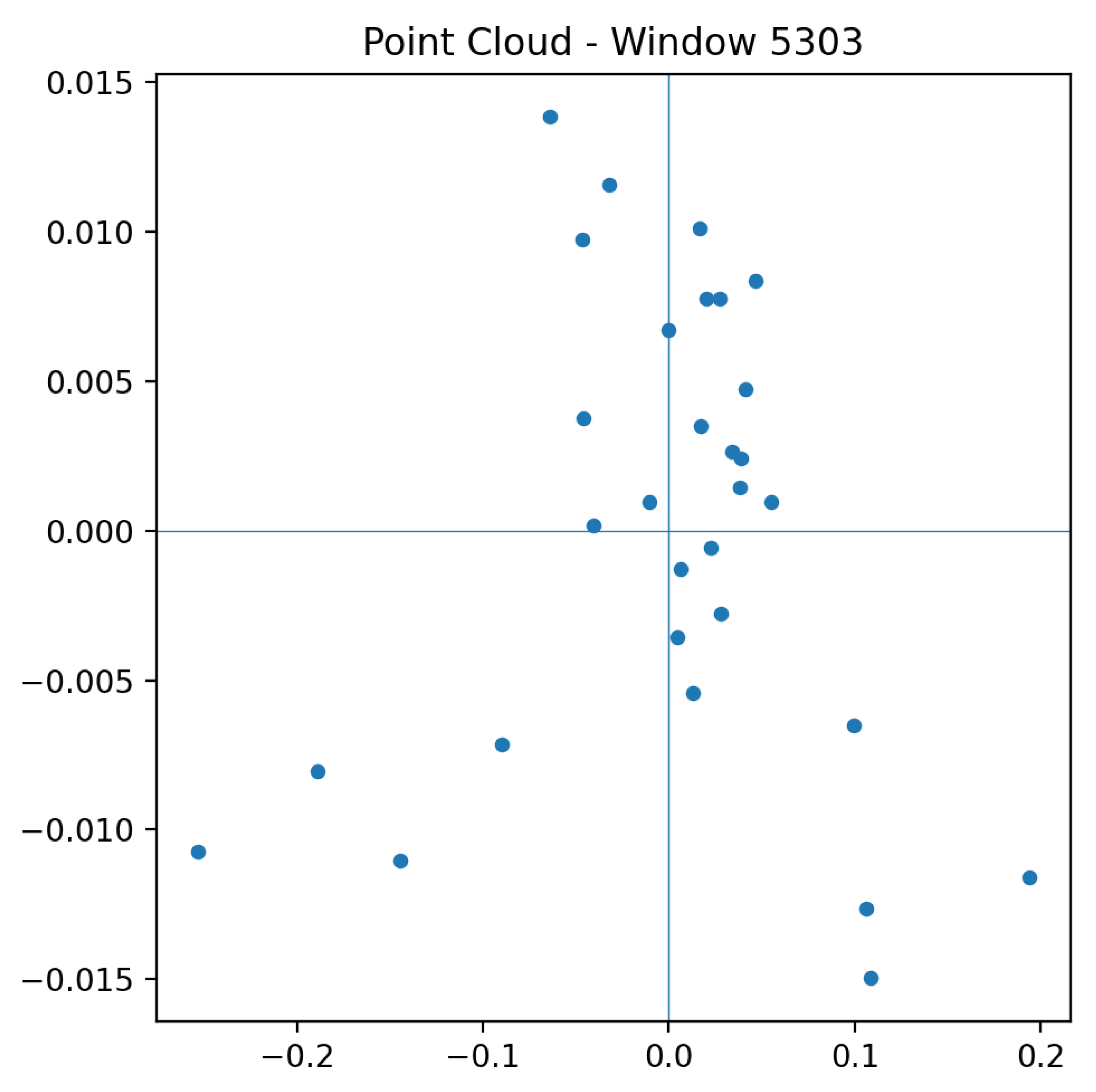
Using a sliding window of $w=30$ trading days, we generate 5506 overlapping point clouds in ${\mathbb{R}}^4$. Each cloud encodes the joint behaviour of the indices during a short horizon. For visualization purposes, clouds may be projected into lower dimensions using Principal Component Analysis (PCA), though persistent homology is computed in the full four-dimensional space. Figure 2 and Figure 3 show representative point clouds for both stable and turbulent market periods.

4.2. Crisis Labeling and Ground Truth

Ground truth crisis periods are defined using a hybrid strategy. First, four canonical systemic events are identified: the dot-com bubble (2000), the global financial crisis (2008), the US sovereign debt downgrade (2011), and the COVID-19 crash (2020). These are well-established crises in financial history and serve as reference benchmarks.

Second, to reduce reliance on purely historical annotation, we add a quantitative rule: periods are labeled as crises if realized volatility exceeds the 95th percentile of its historical rolling distribution. This dual approach balances interpretability with reproducibility and helps capture periods of exceptional stress that may not fit neatly into the four canonical events.

4.3. Topological Feature Extraction

Each point cloud is transformed into a Vietoris–Rips complex using the giotto-tda library, with maximum filtration value $r=0.15$ and Euclidean distance as the metric. Homology groups $H_0$ (connected components) and $H_1$ (loops) are computed.

Persistence diagrams are obtained with the VietorisRipsPersistence transformer. They encode the birth and death of topological features as the filtration radius grows. Points close to the diagonal correspond to short-lived, noisy features, while points far from the diagonal reflect persistent structures. Figure 4 and Figure 5 illustrate persistence diagrams for a stable and a turbulent period, highlighting how crises yield longer-lived features.

Persistence barcodes offer a complementary visualization by representing feature lifetimes as horizontal line segments. Longer bars correspond to persistent components or loops, while shorter bars represent transient features likely attributable to noise. Figure 6 and Figure 7 show barcodes for the same windows as above, confirming the structural differences between stable and crisis periods.

For statistical analysis, persistence diagrams are mapped into persistence landscapes using the PersistenceLandscape transformer, with five layers and 100 bins. Landscapes convert discrete diagram points into functional summaries of persistence. Scalar indicators are derived by computing $L^1$ and $L^2$ norms:

$${\parallel \lambda \parallel }_p={\left(\sum _{k=1}^{\infty }{\int }_{-\infty }^{\infty }\lambda {(k,t)}^{p}dt\right)}^{1/p}.$$

(17)

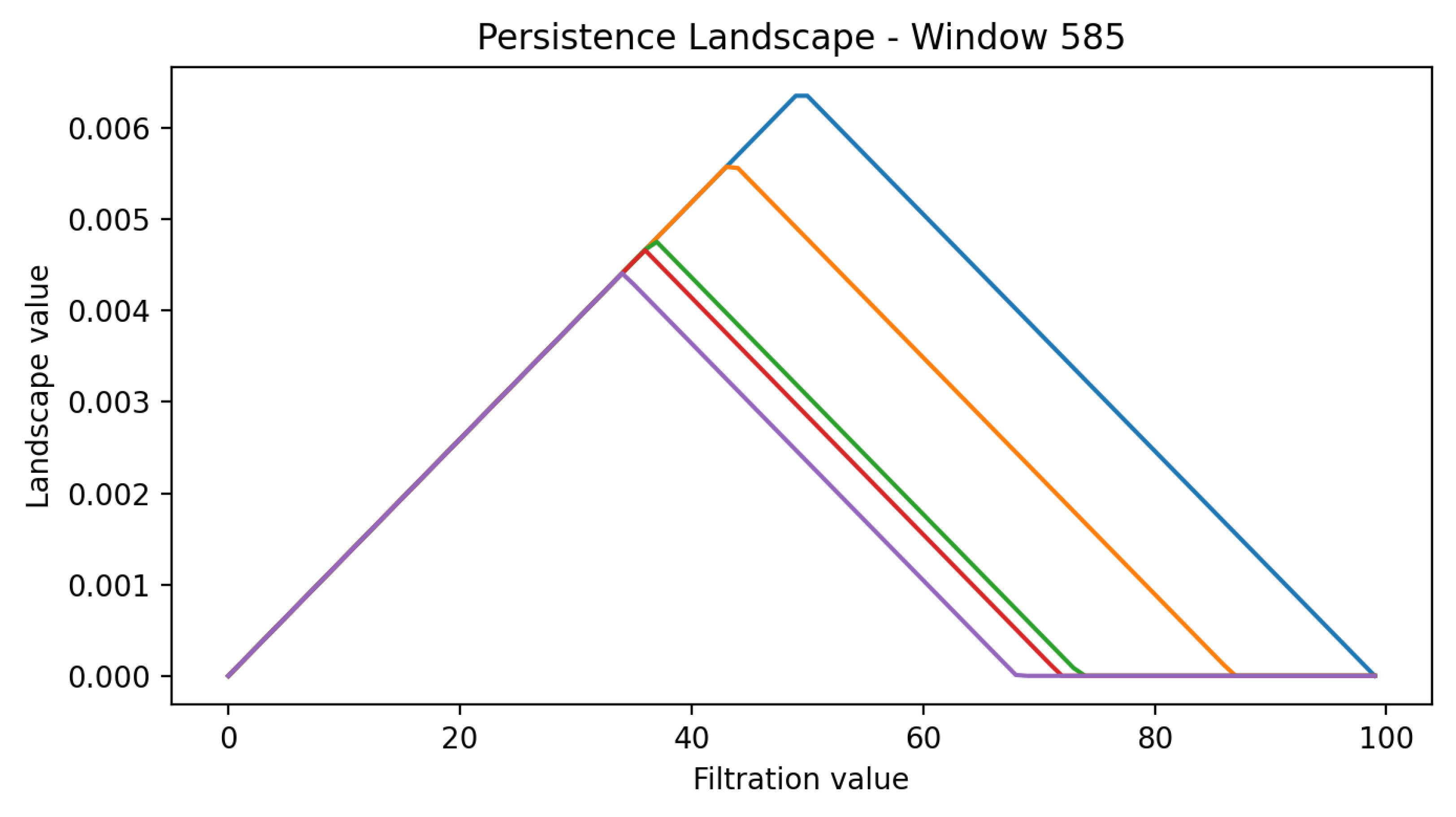
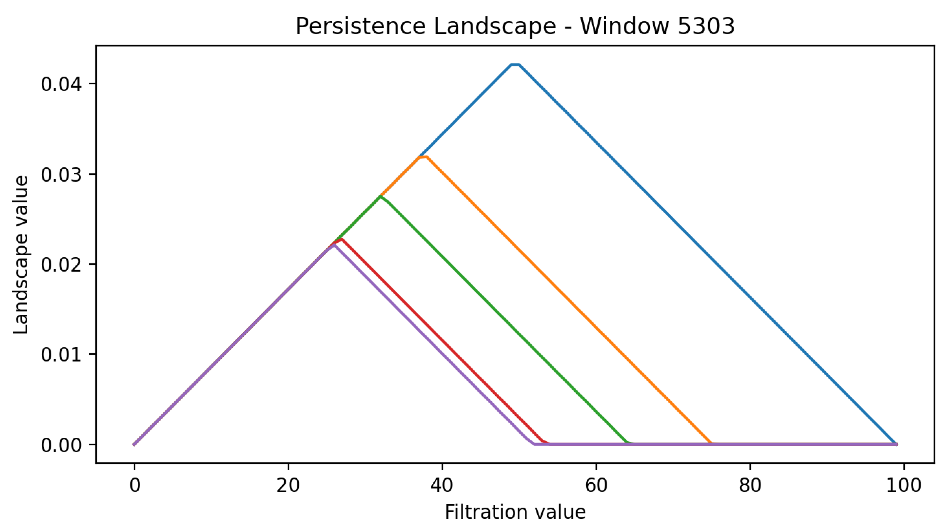
In Figure 8 and Figure 9, the coloured curves are the first layers of the persistence landscape computed on the shown rolling window. Given a persistence diagram, $\lambda (k,t)$ encodes, at filtration value t, the magnitude of the k-th most persistent homology class: lower layers (small k) capture dominant, long-lived features, while higher layers represent progressively weaker features. The x-axis reports the filtration value and the y-axis the landscape amplitude. We plot the first five layers to highlight regime differences: windows preceding crises exhibit taller and broader peaks across multiple layers, whereas tranquil windows display flatter profiles.

4.4. Causal Detection of Early Warning Signals

The norm time series extracted from persistence landscapes is processed through a strictly causal detection rule, ensuring that only past information informs decisions. At each time j, three conditions are applied:

(i)

Sudden local increase: ${\displaystyle \frac{N_j}{N_{j-1}}\ge \alpha }$,

(ii)

Short-term deviation: ${\displaystyle \frac{N_j}{Q_j^{\left(s\right)}}\ge \beta }$, where $Q_j^{\left(s\right)}$ is the mean of the past s values,

(iii)

Sustained elevation: ${\displaystyle \frac{Q_j^{\left(s\right)}}{Q_j^{\left(t\right)}}\ge \beta }$, where $Q_j^{\left(t\right)}$ is the mean of the past t values.

If all conditions are satisfied, j is flagged as the onset of an early warning signal. Consecutive detections are collapsed into single bursts to avoid redundancy.

Detected signals are compared with ground truth crises under the following rules:

• True positive (TP): signal within a 180-day lead window before a crisis,
• Late detection: signal within a 30-day lag window after a crisis,
• False positive (FP): signal outside lead/lag windows,
• False negative (FN): crisis with no associated signal.

From these, we compute Precision, Recall, and F1. Additional indicators include the false alarm rate (FAR), mean lead time, and mean delay time.

The contribution of each component of the pipeline is quantified through an ablation study. Holding the dataset, sliding window, and detector parameters fixed $(\alpha =3.1,\beta =3.1,s=57,t=16)$, we vary one factor at a time: the norm (L1 vs. L2), the homology content (H₀ vs. H₁), the topological summary (landscape vs. raw diagram sum vs. persistence image), and each causal condition (local jump, short-term deviation, sustained elevation), with/without burst collapsing. Signals are matched to canonical crisis onsets using a 180-day lead window and a 30-day late window. Event counts (TP/Late/FN/FP), total signals, precision, recall, F1, false-alarm rate, and mean lead/late times (

Table 2. Ablation study.

Variant	TP	Late	FN	FP	Signals	Precision	Recall	F1 Score	False Alarm Rate	Mean Lead Time	Mean Delay Time
Full (L2, causal i–iii, bursts)	2	0	2	2	4	0.500000	0.500000	0.500000	0.500000	33.500000	0.000000
L1 instead of L2	2	1	1	5	8	0.250000	0.500000	0.333000	0.625000	33.500000	18.000000
H0 only	2	0	2	2	4	0.500000	0.500000	0.500000	0.500000	33.500000	0.000000
H1 only	2	0	2	29	31	0.065000	0.500000	0.114000	0.935000	148.500000	0.000000
Raw diagram sum	0	0	4	0	0	0.000000	0.000000	0.000000	0.000000	0.000000	0.000000
Persistence image + causal detector	0	0	4	0	0	0.000000	0.000000	0.000000	0.000000	0.000000	0.000000
w/o cond (i)	2	1	1	4	7	0.286000	0.500000	0.364000	0.571000	33.500000	11.000000
w/o cond (ii)	2	0	2	2	4	0.500000	0.500000	0.500000	0.500000	33.500000	0.000000
w/o cond (iii)	2	0	2	9	11	0.182000	0.500000	0.267000	0.818000	33.500000	0.000000
no burst collapsing	2	0	2	2	4	0.500000	0.500000	0.500000	0.500000	33.500000	0.000000

) are reported. All indicators are finite (no NaN/Inf).

As per Table 2, the full pipeline (landscape + L2, causal conditions i–iii with burst collapsing) balances anticipation and selectivity (F1 $=0.50$, mean lead $\approx 34$ days). Removing the local jump condition (i) reduces precision (more spurious day-to-day spikes pass through), while removing sustained elevation (iii) yields the largest precision drop, confirming both filters are important. The short-term deviation (ii) is comparatively less influential on this dataset. Regarding topological content, H₀-only nearly matches the full pipeline, whereas H₁-only generates many false positives, indicating connectivity features dominate loop structure for these point clouds. As negative controls, the raw diagram sum and the persistence image produce no warnings under the same strict causal detector, underscoring the stability of persistence landscapes for this task.

4.4.1. Baselines

Realized-volatility thresholds (global and rolling) and a simple TDA+critical-slowing-down hybrid do not outperform the causal TDA pipeline (

Table 3. Baselines and comparators.

Method	TP	Late	FN	FP	Signals	Precision	Recall	F1 Score	False Alarm Rate	Mean Lead Time	Mean Delay Time
Realized vol 95th	0	3	1	10	13	0.000000	0.000000	0.000000	0.769000	0.000000	12.667000
Realized vol (rolling 95th)	2	2	0	31	35	0.057000	0.500000	0.103000	0.886000	30.000000	7.500000
Toponorm non-causal (95th, L2)	1	3	0	10	14	0.071000	0.250000	0.111000	0.714000	66.000000	11.667000
TDA + CSD hybrid	0	0	4	0	0	0.000000	0.000000	0.000000	0.000000	0.000000	0.000000
Persistence image + causal	0	0	4	0	0	0.000000	0.000000	0.000000	0.000000	0.000000	0.000000

. A non-causal toponorm threshold attains some recall but with worse precision and a higher false-alarm rate. These comparisons highlight that (i) the landscape normalization and (ii) the causal detection logic are key drivers of performance.

4.4.2. Qualitative Evidence

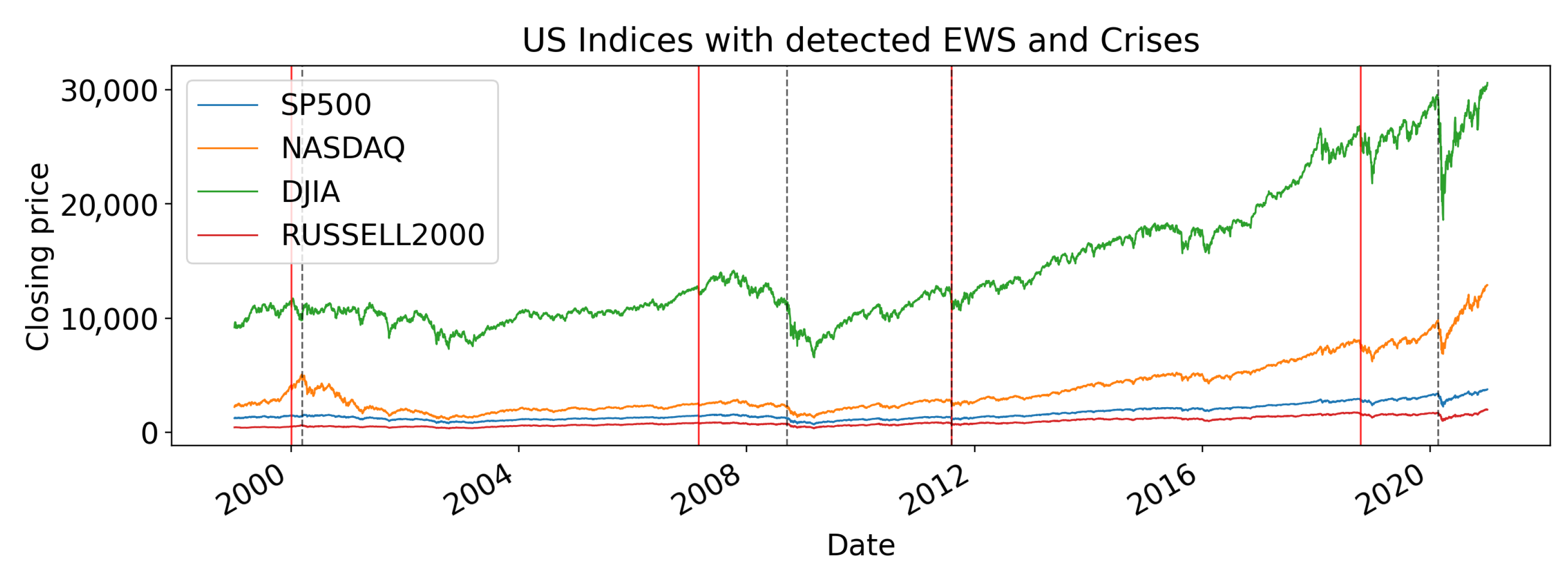
Figure 10 and Figure 11 provide the underlying series and log-returns. Figure 12, Figure 13 and Figure 14 show that warnings occur near major build-ups in the landscape norms, while Figure 15 situates the selected early warnings on the price trajectories alongside crisis onsets.

5. Discussion

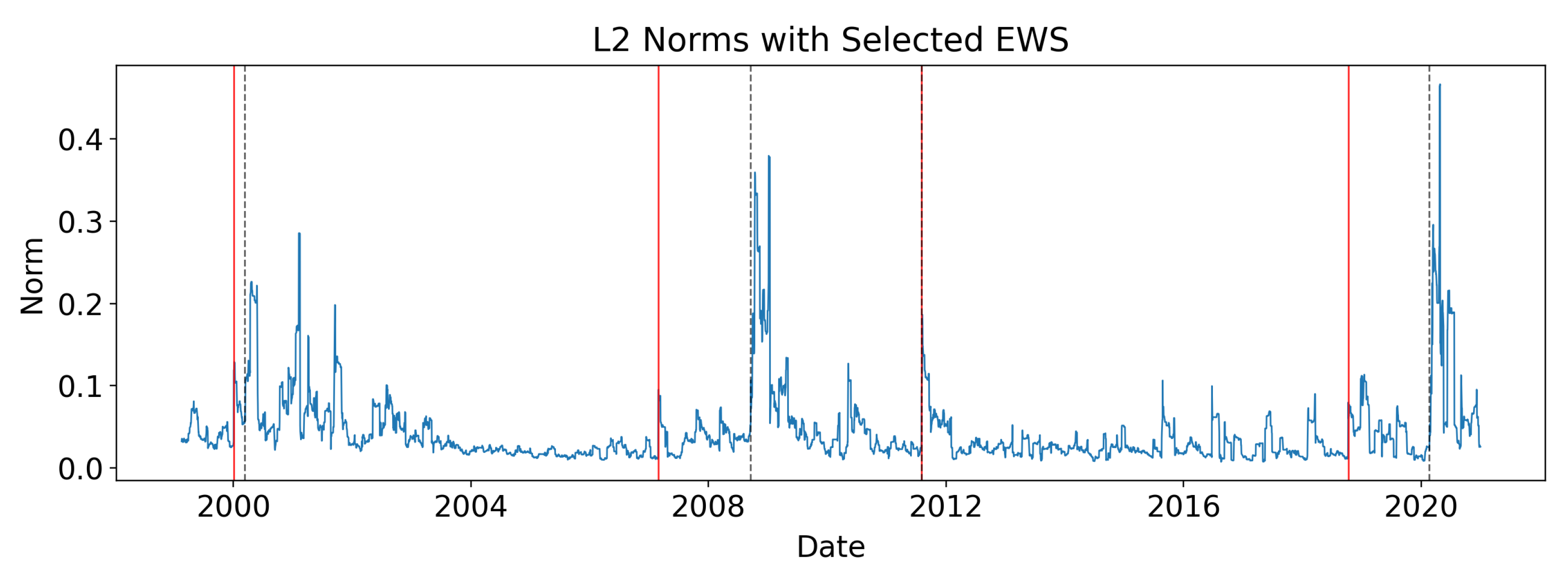
Figure 16 shows the $L^2$ norm series with detected signals. Spikes in the topological indicators cluster around known crises and often appear months in advance, suggesting that persistent homology captures structural changes in market co-movements before conventional stress measures. This anticipatory ability is crucial for systemic risk monitoring, as it provides decision-makers with valuable lead time for intervention.

At the strictly causal operating point used throughout ($\alpha$ = 3.1, $\beta$ = 3.1, s = 57, t = 16), the aggregate performance is $F_1\approx 0.50$ with a mean lead time of about 34 days (Table 2). This reflects a conservative decision rule that balances anticipation and selectivity under identical scoring across all variants.

5.1. Sensitivity Analysis

To probe robustness, we consider two complementary views. (i) For the strictly causal detector, varying $(\alpha ,\beta )$ traces the usual precision–recall trade-off (Figure 17), with recall higher at permissive settings and precision improving as thresholds tighten. (ii) As a permissive baseline, we also examine a simple spike detector controlled by a single z-score threshold $\tau$;

Table 4. Spike baseline sensitivity across z-score thresholds $\tau$. Low $\tau$ ensures high recall but causes frequent false alarms; high $\tau$ reduces false positives but misses events. Intermediate values ($\tau =2.0$–$2.5$) achieve the best trade-off for this baseline, albeit with small absolute $F_1$ values.

Threshold $\mathit{\tau }$	Detections	TP	Late	FN	FP	Precision	Recall	${\mathit{F}}_1$	FAR
1.5	775	4	0	0	771	0.005	1.00	0.010	0.995
2.0	382	3	1	0	378	0.008	0.75	0.016	0.990
2.5	182	3	0	1	179	0.016	0.75	0.032	0.984
3.0	84	1	1	2	82	0.012	0.25	0.023	0.976

reports its behaviour as $\tau$ varies (1.5–3.0), showing the expected reduction in false alarms at the cost of lower recall at stricter thresholds. These results are methodologically distinct from the causal detector and are reported for context.

Figure 17 (spike baseline) shows that recall remains high at low-to-intermediate thresholds, while precision increases as $\tau$ tightens. This illustrates the central trade-off: permissive settings capture most events but issue many false alarms, whereas stricter settings suppress noise but risk missing events.

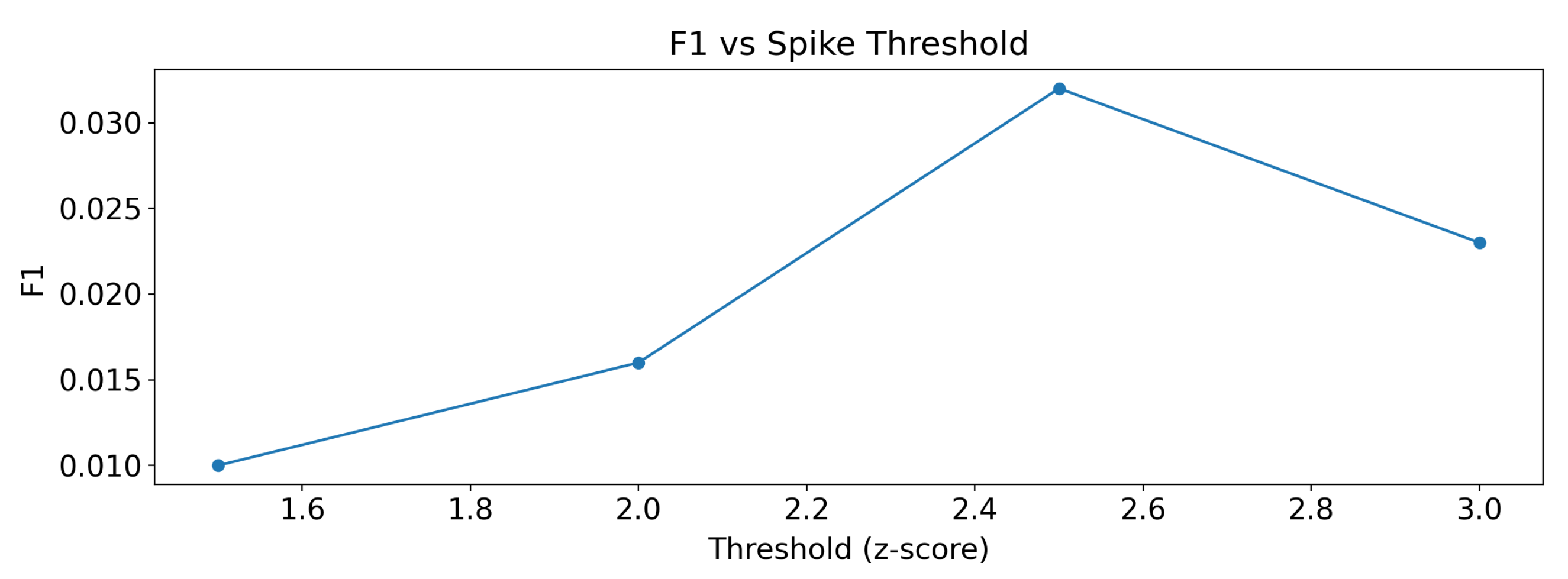
Figure 18 complements this view by plotting the $F_1$ score for the spike baseline. The curve exhibits a modest maximum around $\tau \approx 2.0$–$2.5$; however, absolute $F_1$ values remain small, consistent with the large number of false alarms at permissive settings.

5.2. Validation Against External Indicators

Validation against independent benchmarks is crucial. Using the VIX index with spikes above 43 as markers of extreme volatility, four stress episodes are identified (2001, 2008, 2011, 2020). Figure 19 and Figure 20 show that all episodes are anticipated by the topological signals, with no false positives or late detections.

Figure 19 demonstrates close alignment with VIX spikes: every extreme volatility episode is preceded by a topological signal, confirming that the method detects systemic stress in advance.

Figure 20 provides a more permissive alignment, showing that even beyond the strict spike threshold, topological warnings consistently lead to VIX surges. This highlights the anticipatory character of the signals relative to a widely used benchmark of market stress.

5.3. Comparison with Literature

We re-implemented the core ideas that recur in prior work and evaluated them under the same strictly causal protocol (180-day lead, 30-day late window, identical crisis calendar):

(a)

TDA landscape norms as early signals (e.g., pre-crash rises in $L^p$ norms): already the backbone of our method; we keep the landscape summary but evaluate it with a formal, causal event detector.

(b)

TDA + critical slowing down (CSD) trend–based ideas (e.g., high AR(1)/variance together with a topological signal): implemented as a hybrid baseline (high realized volatility ∧ high AR(1)∧ high toponorm).

(c)

Conventional financial EWS used in the crisis literature: (i) realized-volatility exceedance at a global 95th percentile and (ii) a rolling 95th-percentile realized-volatility rule.

(d)

Controls within TDA to probe representation choice: a non-causal toponorm threshold (95th) and a persistence-image+causal variant.

Under identical settings, the proposed pipeline (landscape $L_2$ + causal conditions with burst collapsing) achieves a balanced precision–recall with F1 = 0.50 and a mean lead of ≈34 days. In contrast:

• Realized-volatility thresholds (global and rolling) and the TDA+CSD hybrid do not anticipate crises under the strict causal scoring (F1 $\approx 0$ in our dataset).
• The non-causal toponorm threshold recovers some recall but at the cost of many false alarms (e.g., Precision $\approx 0.07$, Recall $\approx 0.25$, F1$\approx 0.11$).
• The persistence-image + causal control rarely triggers, reinforcing that persistence landscapes are the more effective summary here.

The comparison highlights and contributions are, therefore, the following:

• Causal event detection and accounting. Prior TDA work often reports pre-crash trends; we formalize a strictly causal detector (local jump, short-term deviation, sustained elevation, and burst collapsing) and report TP/Late/FN/FP with per-crisis matches (CSV provided), enabling transparent benchmarking rather than relying on visual inspection alone.
• Representation choice matters. Persistence landscapes yield selective, auditable warnings; persistence images and raw diagram sums act as negative controls under the same detector.
• Module-level evidence. Results show that $H_0$ features and conditions (i) and (iii) contribute most to precision on this dataset.

Finally, with regard to the limitations of this work, it is possible to see that the number of canonical crises is small; results depend on dating conventions and the lead/late windows (fixed ex-ante for all methods). On these US equity indices, $H_1$ carries less predictive value than $H_0$; we caution against over-generalizing that finding to other markets.

6. Conclusions

This work introduced a strictly causal early–warning framework for financial crises that extracts topological signals from multivariate return streams. Sliding windows of daily log–returns are embedded as point clouds, Vietoris–Rips persistent homology is computed, and persistence landscapes provide an interpretable summary whose $L_2$ norm acts as a single scalar indicator. A simple, transparent decision rule—parameterised by $(\alpha ,\beta )$ and run–length controls $(s,t)$—suppresses isolated spikes and collapses bursts into time–stamped warnings, yielding a pipeline that is auditable end–to–end.

On four major U.S. equity indices (S&P 500, NASDAQ, DJIA, Russell 2000) over 1999–2021, the method attains, at a fixed strictly causal operating point $(\alpha =\beta =3.1,s=57,t=16)$, a balanced precision–recall ($F_1\approx 0.50$) with an average lead time of about 34 days. It anticipates two of the four canonical crises and issues a contemporaneous signal for the 2008 global financial crisis. Sensitivity analyses show that varying $(\alpha ,\beta )$ traces the expected precision–recall trade–off without altering the qualitative behaviour of the detector, while an external alignment against VIX spikes corroborates the anticipatory content of the signals.

Ablation studies clarify the contribution of each stage. The full pipeline—landscape summary with $L_2$ norm, causal conditions (i–iii), and burst collapsing—dominates simplified variants. Removing individual causal conditions increases false alarms; using $L_1$ instead of $L_2$ reduces discrimination; restricting to a single homology dimension ($H_0$ or $H_1$ only) degrades performance, with $H_1$ alone producing many spurious detections. Raw diagram aggregates and persistence–image baselines are weaker under the same scoring. Against non–topological comparators (e.g., realised–volatility thresholds or permissive spike rules), the causal topological pipeline achieves substantially fewer false alarms at comparable recall.

The approach is interpretable: landscape layers visualise the emergence and growth of topological features within a window, while the norm condenses this multi–layer structure into a transparent time series of geometric stress. The resulting warnings are therefore traceable both to specific windows and to visible changes in the shape of the data.

The present study is confined to U.S. equity indices at daily frequency and a fixed window length; results may vary across assets, horizons, and market microstructures. Crisis labels carry inherent dating uncertainty, and the small number of major events limits statistical power. The detector is threshold–based rather than probabilistic and is not evaluated as a trading strategy. Future work will extend the analysis to cross–asset and cross–market settings, explore multiscale and adaptive windowing, investigate alternative filtrations and distances, and integrate calibrated learners (e.g., conformal or Bayesian post–processing) for probabilistic warning scores. Formal uncertainty quantification for topological summaries and tighter couplings with macro–financial covariates are also promising directions.