Article

Self-Adaptive Evolutionary Info Variational Autoencoder

Department of Aeronautical and Automotive Engineering, Loughborough University, Loughborough LE11 3TU, UK
*
Authors to whom correspondence should be addressed.
Computers 2024, 13(8), 214; https://doi.org/10.3390/computers13080214
Submission received: 28 June 2024 / Revised: 12 August 2024 / Accepted: 21 August 2024 / Published: 22 August 2024

Abstract

:
With the advent of increasingly powerful machine learning algorithms and the ability to rapidly obtain accurate aerodynamic performance data, there has been a steady rise in the use of algorithms for automated aerodynamic design optimisation. However, long training times, high-dimensional design spaces and rapid geometry alteration pose barriers to this becoming an efficient and worthwhile process. The variational autoencoder (VAE) is a probabilistic generative model capable of learning a low-dimensional representation of high-dimensional input data. Despite their impressive power, VAEs suffer from several issues, resulting in poor model performance and limiting optimisation capability. Several approaches have been proposed in attempts to fix these issues. This study combines the approaches of loss function modification with evolutionary hyperparameter tuning, introducing a new self-adaptive evolutionary info variational autoencoder (SA-eInfoVAE). The proposed model is validated against previous models on the MNIST handwritten digits dataset, assessing the total model performance. The proposed model is then applied to an aircraft image dataset to assess the applicability and complications involved with complex datasets such as those used for aerodynamic design optimisation. The results obtained on the MNIST dataset show improved inference in conjunction with increased generative and reconstructive performance. This is validated through a thorough comparison against baseline models, including quantitative metrics reconstruction error, loss function calculation and disentanglement percentage. A number of qualitative image plots provide further comparison of the generative and reconstructive performance, as well as the strength of latent encodings. Furthermore, the results on the aircraft image dataset show the proposed model can produce high-quality reconstructions and latent encodings. The analysis suggests, given a high-quality dataset and optimal network structure, the proposed model is capable of outperforming the current VAE models, reducing the training time cost and improving the quality of automated aerodynamic design optimisation.

1. Introduction

As machine learning algorithms continue to develop into powerful tools, they have become increasingly capable in aiding aerodynamic design optimisation. Many different algorithms have shown promise in solving the physical governing equations of aerodynamics and producing accurate predictions based on these, provided the model is well trained with sufficient high-quality data. In their review of machine learning applications in aerodynamic shape optimisation, Li et al. address three key use cases for these algorithms: compacting the geometric design space, fast aerodynamic analysis and efficient optimisation architecture [1]. This study focuses on the variational autoencoder (VAE), a generative probabilistic model capable of inferring a low-dimensional representation of high-dimensional datasets [2,3,4]. Therefore, this work falls within the remit of design space compression, although the VAE has also been applied successfully to the other two use cases.
Saha et al. [5] demonstrate that the VAE can become an extremely powerful tool, successfully training a point cloud VAE capable of generating 3D vehicle geometries. In conjunction, they use computational fluid dynamics (CFD) to analyse the performance of the original vehicle models, combining the data into a multi-layer perceptron. This secondary network maps the performance data to the respective geometry, allowing the network to predict the performance of new samples generated by the VAE. The authors integrate both networks into a simple user interface, within which, the latent variables of the model can be manipulated, altering the design in almost real time. Performance data predictions, provided by the secondary network, are provided in the same time frame, resulting in a rapid generative analysis tool for vehicle design. Rios et al. [6] also successfully implement the VAE to obtain a low-dimensional representation of the design space for a series of 3D vehicles. The authors show that the low-dimensional representation and generative capabilities increased performance when they performed automated aerodynamic design optimisation using CFD. In addition, Mroesk et al. [7] introduce the VAE + I model, which combines a β -VAE model with an interpolation model. The model is trained on different geometry permutations of the DrivAer model and the corresponding CFD data. After successful training, the VAE + I model was able to accurately predict the velocity field of a given geometry after interpolation of the latent variables. Figure 1 presents a workflow outlining the general idea and methods behind using the VAE as part of an automated aerodynamic optimisation problem.
Although VAEs have already been proven as an extremely powerful tool, they face issues, largely because they balance the conflicting objectives of inference and reconstructive performance. It has been observed that the standard VAE struggles to learn a disentangled representation of the data on simple datasets such as MNIST [8]. Further issues, including the information preference problem, modelling bias and dynamic uncertainty, have also been observed in previous research. Attempts to rectify these issues have led to a number of different models being proposed. The main approaches, such as β -VAE and InfoVAE, introduce hyperparameters to improve the balance between reconstruction and inference [8,9]. Other approaches have also emerged, such as ControlVAE, a VAE model that actively tunes the beta hyperparameter through proportional–integral–derivative (PID) control [10]. Despite these efforts, recent research reveals that these modifications are still insufficient in balancing the trade-off between reconstruction and inference. Furthermore, these models require tuning of the hyperparameters to achieve optimal performance, significantly reducing the algorithm’s attractiveness for fast and efficient optimisation, given the current tuning methods. Recently, eVAE has been introduced, and this model uses evolutionary processes for the optimisation of the VAE and its hyperparameters. The model jointly tackles the random search problem associated with hyperparameter tuning and VAE performance issues.
Evidently, VAE is not the only solution to computer vision and generative image modelling. Generative adversarial network (GAN) models are particularly popular for image generation and are often directly compared to VAE models. The GAN model utilises an entirely different framework, employing two models, a generator and a discriminator, pitted against each other in a form of minimax game. Due to their nature, as the discriminator improves, the gradients become increasingly small, often causing divergence and significant instability in the training [11]. Despite these issues, GAN models have successfully been applied to design problems, such as the study into non-pneumatic tire pattern design conducted by Seong et al. [12]. Another successful method for image generation and restoration is random field-based models, which use local pixels to estimate unknown or noisy pixels, hence enabling them to both restore and improve the quality of images. Andriyanov et al. [13] employ this to successfully restore satellite images, even when 50% of the original information has been artificially removed. Several GAN models have been proposed for the purposes of shape parameterisation and aerodynamic design optimisation of aerofoils [14,15,16]. Perhaps the best of these is AirfoilGAN, a framework based on VAEGAN [17], proposed by Wang et al. [18]. The AirfoilGAN model combines the VAE and GAN models by implementing the encoder-decoder of the VAE as the discriminator of the GAN model. The authors apply the model successfully to 2D aerofoil coordinates, training the network to successfully synthesise novel aerofoil shapes. The aerofoils are analysed in XFoil to find the lift and drag coefficients, and the model then adjusts the shape based on a simple loss function, driving the model to produce aerofoils closer to the target lift and drag coefficients.
It is clear from the literature that there are a number of machine learning models available for generative design and optimisation. VAE is the ideal candidate for these applications due to its dimensionality reduction and ability to learn a meaningful latent encoding. However, it appears that the GAN models currently lead the way in successful application to aerodynamic design optimisation. It is therefore necessary to investigate new VAE models to improve their performance and applicability to the field of aerodynamic design optimisation. This study investigates the possibility of combining ELBO objective modification with evolutionary tuning in an attempt to extract maximal performance in the shortest time frame. This culminates in the new self-adaptive evolutionary info variational autoencoder (SA-eInfoVAE) model and a demonstration of the resulting improvements in performance and time cost. The main contributions of this paper are as follows:
  • We combine the implementation of the InfoVAE model ELBO objective with the evolution strategy of the eVAE model to create a new eInfoVAE model.
  • We improve on the evolution strategy from eVAE, by implementing the higher search power self-adaptive simulated binary crossover, to introduce the novel SA-eInfoVAE model.
  • We comprehensively analyse and validate the improved performance of the proposed SA-eInfoVAE model on the MNIST dataset against existing models. Performance metrics include reconstructive, generative and disentanglement performance and latent encoding strength.
  • We assess the performance of the SA-eInfoVAE model on a complex dataset to determine its applicability and capability to improve on aerodynamic optimisation problems that are being solved using machine learning algorithms.

2. Related Works

2.1. The Variational Autoencoder

The VAE, first introduced by Kingma and Welling [2], combines variational Bayesian methods with the autoencoder structure to create a powerful generative probabilistic model. The algorithm is a latent variable generative model, meaning it models the underlying distribution between an input space x X and a latent space z   Z . The latent space, Z , contains the latent variables, z , which describe the most important factors and dependencies of a complex dataset. For example, three latent variables may be scale, rotation and colour. By learning and manipulating the latent variables, the generative performance can be controlled, i.e., altering the latent variables for rotation only changes the rotation of the output. This is the ideal encoding of the latent variables; more often than not, several factors are encoded into the same latent variable, a poor encoding. Altering the variable in this case changes both the scale and rotation of the object simultaneously, hence showing the model has been unable to disentangle the key features of the data.
In contrast to the original autoencoder, where the latent variables are described by a single discrete value, the latent variables of the VAE are described by a probability distribution. By sampling from the distribution, the value of the latent variable changes, hence producing variation in the generative output. The VAE uses Bayes theorem to learn the posterior distribution p ( z | x ) , which maps the input data, x , to the latent variables, z . To compute the posterior distribution, Equation (1) shows that Bayes theorem requires the likelihood p x ˆ z between the output, x ˆ , and the latent variables, the true prior p ( z ) and the marginal probability, also called the evidence, of the output p ( x ˆ ) .
p z x = p x ˆ z p ( z ) p ( x ˆ )
Unfortunately, in this case, the marginal probability is considered intractable; that is, the integral required to calculate the evidence has no closed form or, in cases where it does, requires an exponential time to compute [19]. Instead, variational inference is used, introducing an approximate posterior distribution q z x , which is then manipulated until it matches closely to—or, in theory, exactly to—the true posterior distribution p ( z | x ) . The approximate posterior distribution is manipulated by the weights of the encoder and decoder that comprise the neural network. In turn, the weights of the network are updated in accordance with the loss function—in this case, the evidence lower bound (ELBO). This is formulated to provide a lower bound estimation to the previously intractable evidence. The ELBO takes the form of Equation (2), assuming an encoder parametrised by weights ϕ and a decoder parametrised by weights θ . It is common to assume that the true prior, p ( z ) , is in the form of a simple distribution, such as the standard normal distribution, and the likelihood is a complex conditional distribution.
L E L B O ( x ) = E q ϕ z x log p θ x ˆ z D K L ( q ϕ ( z | x ) | | p θ z )
In Equation (2) the term D K L represents the Kullback–Liebler (KL) divergence, a statistical measure that determines the difference in information between two distributions. When the KL divergence is zero, the two distributions are identical and therefore represent the same information [20]. The first term in Equation (2) represents the expectation of the output and measures the difference between the ground truth data x and the generated output x ˆ . To ensure varied generation, the VAE randomly samples the distribution q ϕ ( z | x ) , meaning stochastic gradient descent optimisation methods are no longer applicable [21]. To circumvent this issue, the encoder network structure is redesigned to output two parameters for each latent variable, the mean μ and the variance σ . The two parameters describe each probability distribution and, in conjunction with the random sampling, allow the sampled latent variable z * to be representative of the distribution and enable backpropagation through the re-parameterisation trick [2]. Figure 2 details this as part of the overall VAE workflow.

2.2. Issues with Variational Autoencoders

Even though the VAE has proven to be a powerful tool for low-dimensional representation learning of high-dimensional datasets, research shows they suffer from several issues. The first of these issues relates to the fact that the approximate posterior distribution inferred by the model is often far from the true posterior distribution in the data, meaning the model learns a poor representation of the data. There are two primary reasons for this: the first relates to the nature of the ELBO objective itself, and the second is due to the difference in dimensional scale between the input and the latent variables. Regarding the first issue, Zhao et al. detail how the regularisation term ( D K L ) in the ELBO objective fails to stop the ELBO from being optimised. The authors prove mathematically that the estimation of the evidence can be maximised when the approximate posterior q ϕ z x and true posterior p θ ( z | x ) are distant, even infinitely far apart [9]. In these cases, the model appears to achieve an optimal solution, when, in reality, the model has completely failed to infer the underlying distributions of the data. Learning a poor representation of the data cripples the performance of the VAE, generating outputs that in no way relate to the input data. Modelling bias is another cause of poor model inference, a phenomenon caused by significant differences in dimensionality between the input and the latent variables. Consequently, when maximising the ELBO objective, the input incurs a much larger per dimensional modelling error. This encourages the model to sacrifice minimising the divergences in the latent space Z to instead minimise the divergence of the input space X and the reconstructive error. As a result, the model fails to learn a good approximation to the true posterior distribution, resulting in poor latent variable encodings and suboptimal model performance.
VAEs also suffer from the information preference problem, which encourages the model to completely ignore the latent variables. This issue typically arises when a powerful decoder network is used, allowing the likelihood distribution to become significantly flexible [22]. Generally, a powerful decoder is required when high-quality sample images are required from a complex natural image dataset, as is the case in many applications of the VAE [9]. Two examples of such decoders are PixelRNN [23] and PixelVAE [24]; both models are specifically designed for modelling the distribution of natural images and generating high-quality samples as a result. Due to the large amount of flexibility in the decoding distribution, p θ x ˆ z becomes the same for all latent variables z , and therefore, the input x becomes entirely independent of the latent variables. In this state, the ELBO objective can still be optimised, ignoring the latent variables, generating outputs x ˆ that are all extremely similar, no matter the value of z input into the decoder. As the ELBO objective is optimised, nothing encourages the model to learn the latent variables, resulting in a poor representation of the data in the latent space. This phenomenon is also commonly referred to as “model collapse” and is typically attributed to the KL divergence term reducing to zero [25].
Wu et al. uncovered further issues with the VAE, describing how dynamic uncertainty is caused by optimising the ELBO objective with only a small gap between the posterior and prior distributions [26]. The uncertainty disturbs the trade-off of reconstructive performance and representation learning. By favouring one side of the trade-off over the other, the model produces either a weak or strong KL divergence. The former case can lead to KL vanishing, causing the posterior distributions to match the prior closely, crippling the model’s generative capabilities and allowing the model to ignore the latent variables entirely [27]. In the latter case, a strong KL divergence causes an un-optimised ELBO objective and therefore a poor estimation of the likelihood. Concerning models that employ hyperparameters requiring tuning to extract the optimal performance, the authors highlight the issue of random search in large hyperparameter solution spaces. Even a model featuring only one hyperparameter in the ELBO objective can have a wide hyperparameter solution space due to network parameters such as the learning rate, number of latent dimensions and number of training epochs.

2.3. Modified Variational Autoencoder Models

2.3.1. The β -VAE Model

The β -VAE model, proposed by Higgins et al. [8], aims to build on the standard VAE with a model capable of an unsupervised generative approach to learning independent latent factors of variation in unlabeled data. The model introduces the β hyperparameter to the standard VAE ELBO objective, scaling the KL divergence term. The authors state that the hyperparameter limits the capacity of the latent information channel, in turn controlling and encouraging the model to learn the statistically independent latent variables. The resulting β -VAE model takes the form of Equation (3).
L β V A E = E q ϕ ( z | x ) l o g p θ x z β D K L ( q ϕ ( z | x ) | | p z )
The authors test their model on three common datasets for evaluation of the disentanglement performance: CelebA [28], chairs [29] and faces [30]. They compare the β -VAE model against the standard VAE, InfoGAN, an unsupervised generative adversarial network developed by Chen et al. [31], and DC-IGN, standing for deep convolutional inverse graphics network, developed by Kulkarni et al. [32]. The latter is a semi-supervised model, which utilises an architecture similar to that of the VAE, while the InfoGAN model is entirely unsupervised. This provides a state-of-the-art direct comparison to the standard VAE and β -VAE models. The authors go on to show that the β -VAE model significantly outperforms the standard VAE, InfoGAN and DC-IGN, particularly in disentanglement performance. This is particularly advantageous, as both the InfoGAN and DC-IGN models require some form of prior knowledge of the nature of the data’s generative factors.

2.3.2. The InfoVAE Model

The InfoVAE model, as detailed by Zhao et al. [9], aims to avoid the information preference problem and inference failures experienced by the standard variational autoencoder. The authors achieve this by modifying the ELBO objective, introducing the scaling parameter λ to control the divergence between the approximate prior q ϕ ( z ) and the true prior p ( z ) . This aims to counteract the imbalance in dimensionality between the input space X and the latent space Z . A mutual information maximisation term, scaled by the parameter α , is added to encourage the model to favour high levels of mutual information between x and z , hence avoiding the information preference problem [33]. Given these modifications, the ELBO objective takes a new form seen in Equation (4), assuming an encoder parametrised by ϕ and a decoder parametrised by θ , where the term MMD represents the maximum mean discrepancy. The maximum mean discrepancy is a kernel-based statistical measure of the difference between two distributions. Specifically, the metric measures the distance between the means of the two distributions but can also differentiate between distributions with different variances [34].
L I n f o V A E     E q ϕ z x log p θ x z 1 α K L ( q ϕ z x | | p θ z x ) α + λ 1 M M D ( q ϕ ( z ) | | p θ z )
The authors test the InfoVAE model by performing experiments on the MNIST dataset, in the first instance, to demonstrate the InfoVAE model is able to overcome the modelling bias and information preference problem. The authors validate this by presenting a series of probability distribution plots demonstrating the InfoVAE model’s ability to learn a smooth and accurate distribution, while the standard VAE significantly overestimates the distribution. The authors then go on to qualitatively compare generative and reconstructive image samples against the standard VAE, in which the InfoVAE model consistently produces higher-quality images.

2.3.3. The Evolutionary Variational Autoencoder Model

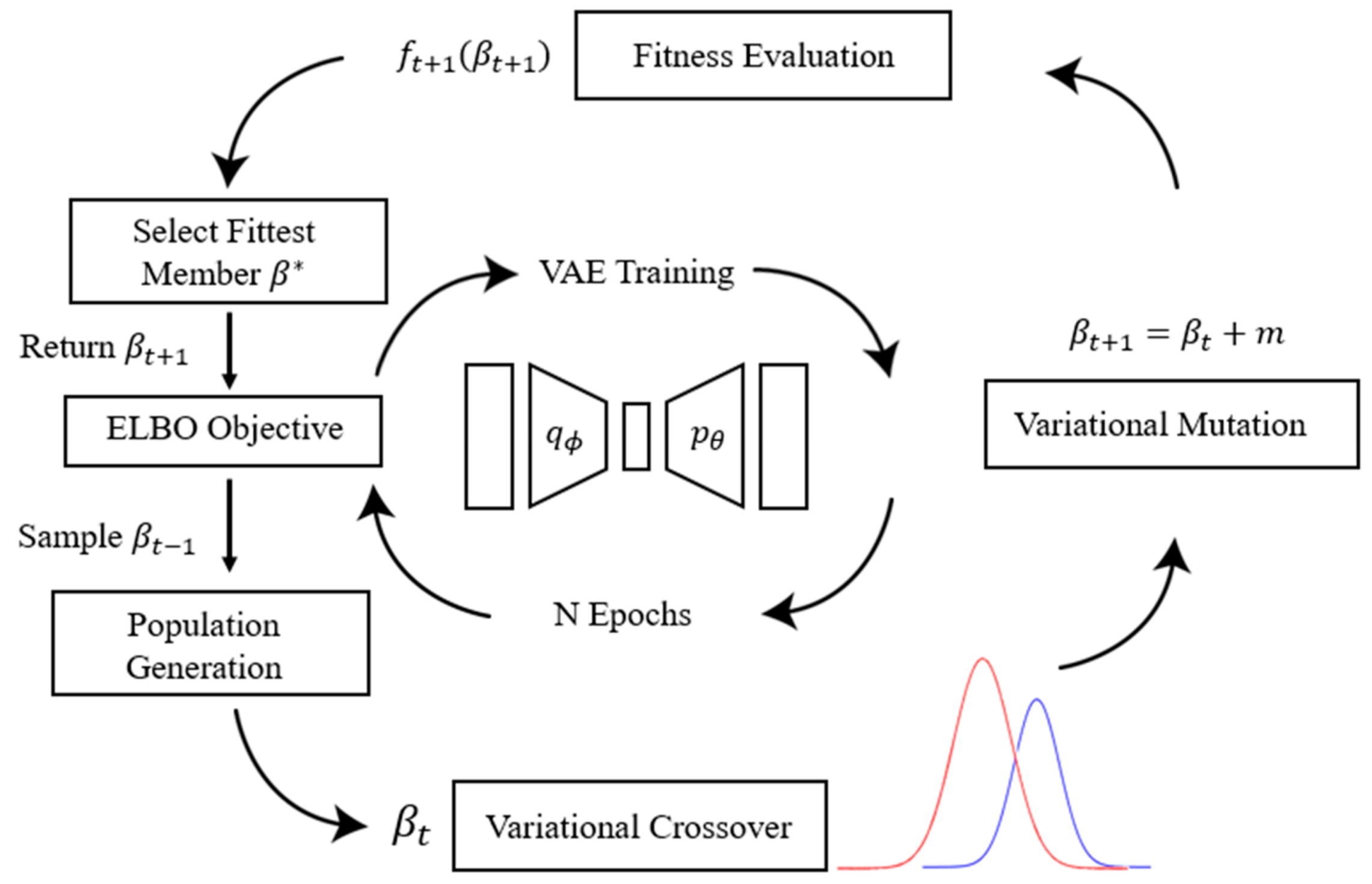
The evolutionary variational autoencoder (eVAE) introduced by Wu et al. [26] addresses the issues faced by VAEs via a different approach. The proposed model aims to address the dynamic uncertainty experienced when optimising the ELBO objective whilst simultaneously tackling the hyperparameter tuning problem. The eVAE framework, shown in Figure 3, operates two loops in an inner–outer architecture, the inner loop training a VAE model and the outer loop performing variational evolutionary processes to tune the hyperparameters of the ELBO objective. The authors choose to apply evolutionary processes to the β -VAE model. The model takes the form of Equation (3), with the added β hyperparameter scaling the KL divergence term. One full cycle of eVAE training involves training the VAE for a specified number of epochs, passing β to the evolutionary outer loop where a population is sampled from a distribution centred on the previous value of β . Each member of the population is assigned a random variable to determine whether it will undergo variational crossover or mutation processes. Once each member of the population has undergone evolutionary processing (or not, in some cases), the new population is evaluated for fitness. The strongest performing member, designated β * , is passed back to the inner loop to continue training the VAE and restarting the cycle. The cycle continues, dynamically updating the β hyperparameter until the value of β converges or another stopping criteria is met. The authors validate the improved performance of the eVAE model in comparative tests against the standard VAE, β -VAE and ControlVAE on the CelebA [28] and dSprites datasets. The authors present a series of loss function graphs, showcasing how eVAE improves the generative performance on the CelebA dataset and gives better disentanglement of the latent factors on dSprites. The authors explore the elementwise KL divergence of these latent factors and present latent traversal plots from the models, exploring qualitatively the strength of the latent encodings. The images demonstrate eVAE’s improved ability to disentangle latent factors, with each row representing an independent latent factor, while the previous models remain much less independent.

2.4. Genetic Algorithms and Evolution Strategies

2.4.1. Simulated Binary Crossover and Cauchy Distributional Mutation

The eVAE model employs variational crossover and mutation operations, specifically simulated binary crossover and Cauchy distributional mutation. Simulated binary crossover (SBX) is a real-coded genetic algorithm developed by Deb and Agrawal that aims to fix issues associated with binary-coded genetic algorithms whilst retaining their search power [35]. Binary-coded genetic algorithms face a number of inherent issues, including those associated with the binary mapping of the problem variables, insufficient precision and the Hamming cliff problem. The latter is an issue of binary coding itself, where two neighbouring numbers have binary encodings that are far apart and require a large number of bits to be flipped to reach the neighbour. The fixed string length of a binary representation has also been shown to limit the precision of a solution, and posing further issues is the fact that the optimal string length is unknown prior to evaluation [35]. Therefore, when the search space is continuous, it is advantageous to use a real-coded genetic algorithm capable of dealing with hyperparameter values directly.
Simulated binary crossover replicates the process of binary single point crossover, a binary genetic algorithm in which a crossover site is selected and two parent binary strings are crossed, generating two new child strings. There are two fundamental properties of binary single point crossover. Firstly, the mean value of the parent strings is the same as the mean value of the child strings after the crossover operation has occurred. Secondly, the parents and children are always equidistant about the midpoint (mean). The crossover process can have three effects: the child solutions become closer and are enclosed by the parents, i.e., contract; the child solutions move further apart and enclose the parent solutions, i.e., expand; or the child solutions remain the same as the parent solutions, a stationary crossover. The authors calculate the probability distribution for expanding, contracting and stationary crossovers of the binary single point crossover and use this to build a matching distribution for the simulated binary crossover operation. They define the process of simulated binary crossover to involve sampling a random number, determining the “spread factor” ( β ) and use this factor to blend the two solutions according to Equation (5) [36].
x 1 n e w = 0.5 1 + β x 1 + 1 β x 2
x 2 n e w = 0.5 1 β x 1 + 1 + β x 2
It can be shown that Equation (5) preserves the properties of the binary single point crossover detailed previously, meaning the search power of the algorithm is maintained. In this sense, Deb and Agrawal successfully translate the binary single point crossover to the real-coded domain. The probability distribution for contracting and expanding distributions is controlled by the exponent η , also called the distribution index. By altering the value of the distribution index, the probability density function can be altered, and small values create a wide distribution, enabling child solutions further from the parents. In contrast, high values create a narrow distribution, allowing for little deviation of the child solutions from the parent solutions. The eVAE model also implements variational mutation; in this case, the authors choose Cauchy distributional mutation, where the mutation is randomly sampled from a Cauchy distribution and added to the value of the hyperparameter.

2.4.2. Self-Adaptive Simulated Binary Crossover

The self-adaptive property proposed by Deb et al. builds on the base operator, introducing a dynamic probability density distribution [37]. As previously discussed, the distribution index, which takes the form of the exponent, controls the spread of the probability distribution and, hence, of the parent and child solutions. The authors note that, when searching a function space for the optimal solution, selecting the appropriate value of the exponent significantly impacts whether it is possible for the function to locate the optimal solution or not. The authors propose the solution to introduce a set of rules to update the exponent dynamically based on the fitness of the child and parent solutions. According to these rules, the distribution index is updated, narrowing when approaching an optimal solution and widening when far from an optimal solution. Through this addition, the search power and precision of the genetic algorithm are increased, providing increased model performance and decreased training time cost.

3. The Self-Adaptive Evolutionary Info Variational Autoencoder Model

The self-adaptive evolutionary info variational autoencoder (SA-eInfoVAE) model combines the ELBO modification of the InfoVAE model with the evolutionary optimisation of the eVAE model. The SA-eInfoVAE model builds on the evolutionary optimisation process of eVAE by using the self-adaptive simulated binary crossover operator and, hence, increased search power. The following sections detail the implementation of the SA-eInfoVAE. The model was implemented in Python using the Google Colab hosted Jupyter Notebook service. The neural networks were implemented using the PyTorch machine learning module, and all results in Section 4 were run on a NVIDIA Tesla T4 GPU, designed specifically for machine learning applications [38]. The implemented code of the SA-eInfoVAE model and the previous baseline models used for comparison are available at the GitHub repository detailed in the Data Availability Statement section.

3.1. Implementation of the InfoVAE ELBO Objective

The first step in implementing the SA-eInfoVAE model is to compute each component of the InfoVAE ELBO objective seen in Equation (4). In Equation (4), the form of the ELBO objective is defined using the probability distributions; however, these are not directly available during training. Therefore, the ELBO objective must be computed in an alternative form. The first term of the InfoVAE ELBO objective ( E q ϕ z x log p θ x z ) measures the reconstruction error between an input x and the reconstructed output x ˆ . The reconstruction error is measured by calculating the pixel-wise mean squared error (MSE), calculating the squared error between input–output pixel pairs and taking the mean over the batch. This process is shown in Equation (6), where ϕ and θ represent the weights of the encoder and decoder, respectively.
L M S E θ , ϕ = 1 N i = 1 N x i f θ g ϕ x i 2
The second term of the ELBO objective measures the KL divergence between the inferred and true posterior distributions, encouraging the model to accurately infer the latent variables of the dataset. Classically, the KL divergence is calculated by finding the expectation of the logarithmic differences between the probability distributions p and q . Unfortunately, in the case of the VAE, this form is not computable due to the network requirements for backpropagation, forcing the distribution to be reconstructed from the mean and variance. It is therefore necessary to modify the KL divergence formula to one that is computable using the values output by the encoder. Equation (7) shows the computable KL divergence formula implemented in the code.
D K L [ q ϕ ( z | x ) | N ~ 0 ,   1 = 0.5 i = 1 N ( 1 + log z σ i 2 z μ i 2 z σ i 2 )
The final term of the ELBO objective is the maximum mean discrepancy between the true and approximate prior distributions. Unlike the KL divergence, the maximum mean discrepancy can be readily computed in the empirical form using the kernel trick [34], where k represents the inverse multiquadric kernel [39], shown in Equation (9). Here, c is the scaling parameter. The maximum mean discrepancy is therefore calculated via Equation (8), where z represents the true prior and z * represents the approximate prior.
D M M D ( q | | p ) = 1 n ( n 1 ) E p z , p z * k z , z * + 1 n ( n 1 ) E q z , q ( z * ) k z , z * 2 n 2 E q z , p z * [ k ( z , z * ) ]
k ( z , z * ) = 1 z z * 2 + c 2
The final aspect of InfoVAE ELBO objective that requires implementation is the re-parameterisation trick, needed to ensure proper backpropagation of gradients through the network. The encoder is structured to output the mean and variance parameters that describe the distribution, while the decoder expects a randomly sampled value of the latent variable. To satisfy these conditions, the re-parametrised variable z * is constructed from the encoder outputs according to Equation (10), where ϵ is sampled randomly from ϵ ~ N ( 0,1 ) .
z i * = μ i + σ i     ϵ

3.2. Implementation of Evolution Strategy

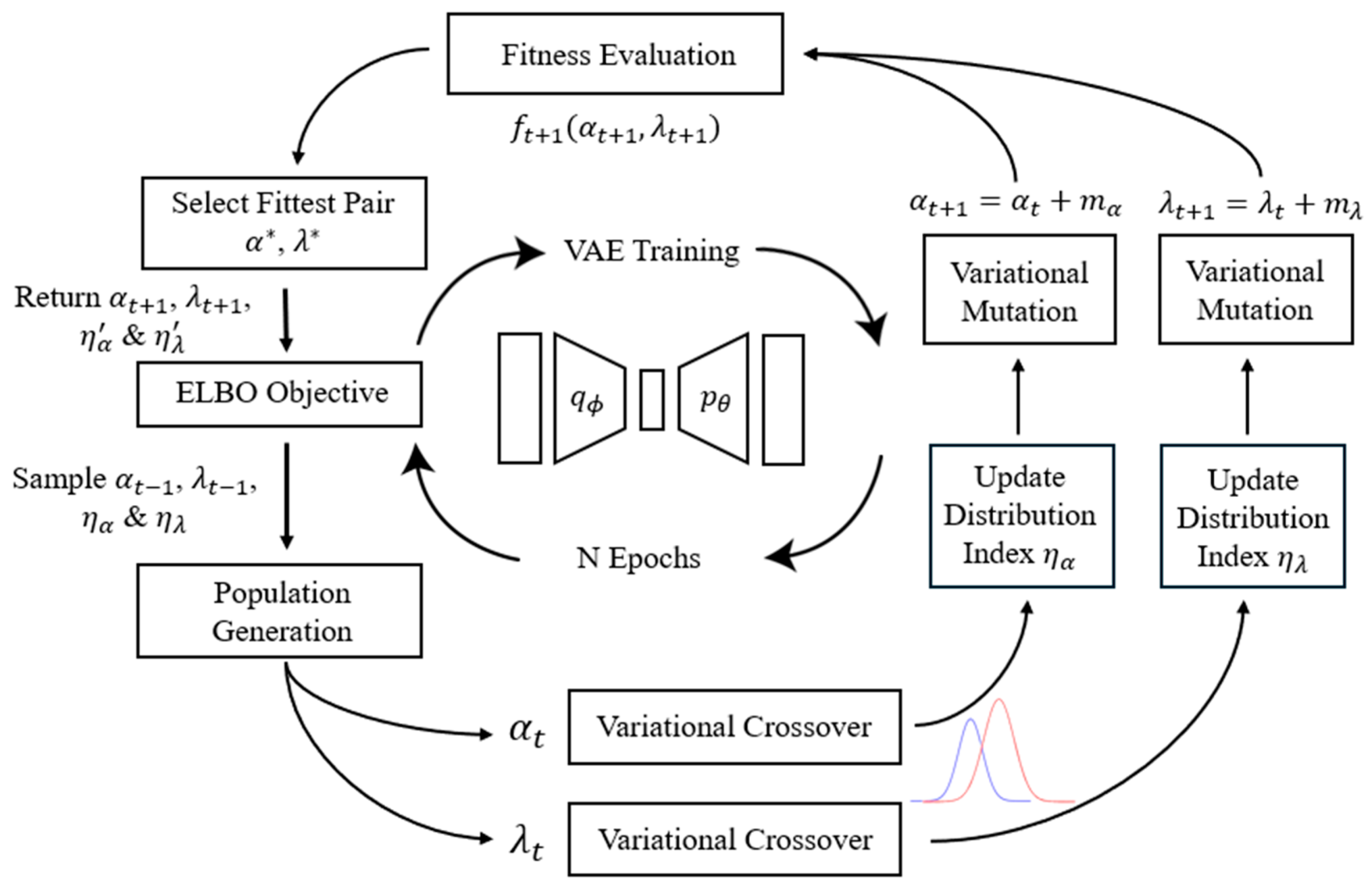
The outer evolutionary loop takes the following order: generate population, sample random variable, determine whether crossover and mutation operations will occur, perform the crossover and mutation operations and evaluate the child solutions for fitness. The fittest pair of hyperparameters from the generation are passed on to the next generation. The InfoVAE ELBO objective contains two hyperparameters ( α and λ ), and both have separate probability distributions and exponents that update individually. The following implementations of self-adaptive simulated binary crossover and Cauchy distributional mutation are shown for the λ scaling parameter but occur for both parameters simultaneously.
The training loop begins by generating a population of “chromosomes” based on the value of λ t 1 passed from the previous round of InfoVAE training. The population is then generated by sampling the given number of the members from a Gaussian distribution λ t ~ N ( λ t 1 ,   1 ) . The crossover and mutation rate parameters are user-defined and allow crossover and mutation when n , sampled randomly from the uniform distribution n     [ 0 ,   1 ] , is less than the mutation or crossover rate. This process occurs for every member of the population. Members that do not undergo evolutionary operations remain perturbed only by the initial sampling distribution. The process for a member undergoing both crossover and mutation operations is outlined below. The first step in the process is to undergo self-adaptive simulated binary crossover, defined by the following steps:
  • Sample u randomly from the uniform distribution u     [ 0 ,   1 ] .
  • Calculate r c from Equation (11) below.
    r c = 2 u 1 η + 1 1 2 1 u 1 η + 1 if   u   0.5 , otherwise
  • Calculate the two child solutions by blending the current population member λ t i with the previous value λ t 1 , shown by Equation (12) below.
    C : λ t + 1 1 = 0.5 · [ 1 + r c λ t i + ( 1 r c ) λ t 1 ] λ t + 1 2 = 0.5 · [ 1 r c λ t i + ( 1 + r c ) λ t 1 ]
  • Evaluate the fitness, f , of both child solutions according to the fitness function in Equation (13) and select the fitter child solution to be passed to the final population.
    f = 1 L I n f o V E ( α t + 1 i , λ t + 1 i )
After the child solution has been selected, the distribution index needs to be updated in accordance with the rules outlined by Deb et al. This allows the probability distribution for the next cycle to be updated in accordance, moving the distribution closer to the optimal solution. The process for this is outlined below:
  • Set the exponent update factor γ λ .
  • Calculate the spread factor β according to Equation (14) below.
    β = 1 + 2 ( λ t + 1 λ t ) ( λ t λ t 1 )
  • Evaluate the fitness of λ t + 1 , λ t and λ t 1 according to the fitness function in Equation (13).
  • Determine whether the child solution lies within the region bounded by the parents or outside of this region. In the latter case, the nearest parent must also be determined.
  • Update the distribution index η using the appropriate equation determined by the following set of rules detailed by Deb et al. [37]. If the child solution lies outside of the region bounded by the parents and is a better solution compared to the nearest parent, the updated distribution index η is calculated using Equation (15) below.
    η   = 1 + η + 1 l o g ( β ) l o g ( 1 + γ β 1 )
  • If the child solution lies outside the region bounded by the parents and is a worse solution compared to the nearest parent, η is calculated using Equation (16) below.
    η   = 1 + ( η + 1 ) l o g ( β ) l o g ( 1 + ( β 1 ) γ )
  • If the child solution lies in the region bounded by the two parents and is a better solution compared to either parent, η is calculated using Equation (17) below.
    η = 1 + η γ 1
  • If the child solution lies in the region bounded by the two parents and is a worse solution compared to either parent, η is calculated using Equation (18) below.
    η = γ 1 + η 1
In all cases, the value of η is limited to the bounds [0, 50], i.e., if η < 0 , the value is reset to 0, and similarly, if η > 50 , the value is reset back to 50. This ensures that the probability distribution determining expansion and contraction and the accompanying equations to determine r c remain meaningful and do not cause the distribution to take an extreme or distorted form. The updated values for η are stored paired with the respective hyperparameter. In cases where the crossover operation does not occur, the current value for the distribution index is passed on, i.e., η = η .
Following the crossover operation is the mutation operation, which simply involves sampling a random variable l from a uniform distribution l   [ 4 ,   4 ] The random variable is then used to sample from the Cauchy distribution described in Equation (19) below.
r m = 1 π ( 1 1 + l 2 )
The value sampled from the Cauchy distribution is then simply added to the value of the hyperparameter to perturb the values further, as seen by Equation (20).
λ t + 1 = λ t + 1 + r m
Once all the crossover and mutation operations have occurred for each member of the population, the new hyperparameters (and distribution indexes) form the final population. This final population is evaluated by the fitness function seen in Equation (13), and the best performing pair of hyperparameters is passed to the inner loop for VAE training, restarting the cycle of the SA-eInfoVAE model. Figure 4 shows the workflow of this implementation.

3.3. Implementation of Qualitative Comparisons and Quantitative Performance Metrics

Due to the nature of the VAE and its variety of applications, there is no single agreed-upon metric to measure the model performance. The following details the implementation of a number of common metrics and comparisons. These are used to ascertain the performance of the proposed and baseline models, providing methods for comparison.

3.3.1. Loss Function Logging and Generated Images

The ELBO objective of the VAE serves as the loss function for iterative optimisation, allowing the weights of the model to update accordingly through backpropagation. The ELBO objective is designed to be minimised; given the same dataset and architecture, it provides an easy way to monitor training and compare model performances. Furthermore, the ELBO objective is composed of three different loss components: the reconstruction loss, KL divergence and the maximum mean discrepancy. Monitoring these individual elements along with the overall value of the loss function can provide significant insight into the performance of the models. “Weights and Biases” is a platform designed to develop and monitor machine learning and artificial intelligence algorithms [40] and was integrated into the code to directly monitor the loss function.
One of the key motivations for using the VAE is the ability to use the trained model for its generative capability. It is therefore crucial to assess the quality of the samples generated by the trained model. This process simply involves sampling each latent variable from the standard normal distribution to build the latent vector and passing it through the trained decoder to receive a string of pixels as the output. Arranging the pixels back into an image provides a gauge of the models’ generative quality, allowing comparison of the performance of different models. The process can be repeated many times to capture a range of outputs across the latent space, offering insight into the models’ encodings.

3.3.2. Reconstructive Performance Metrics

Despite the fact generative performance is a key motivation for using the VAE, it is also imperative to ensure the model can produce high-quality samples, close to those in the original dataset. The easiest way to measure this aspect of model performance is to directly measure the reconstructive performance of a specific input to the model. The process to measure this involves training the model and inputting a specific image into the encoder, hence generating the latent vector. Passing the latent vector through the trained decoder and rearranging the pixels produces a direct reconstruction of the input. The quality of the reconstruction can be measured quantitatively by calculating the pixel-for-pixel square error and dividing by the number of samples to find the mean square error, as per Equation (6). This method can also serve as a qualitative metric; using the same inputs across a range of models allows for comparisons of the image quality.

3.3.3. Visualisation of the Latent Space

Another key motivation for the use of the VAE was the models’ ability to compact a high-dimensional design space into a low-dimensional representation. A well-trained model should have clearly independent latent variables, i.e., each variable encodes only one property, such as rotation or scale. It is possible to manually traverse through a latent variable, changing its value in increments. In doing so, this generates a number of outputs that show how the data have been encoded across the latent space. Constricting the number of latent dimensions to 2 allows traversal of the latent vectors to be visualised in a two-dimensional grid, showcasing where specific inputs are encoded and the strength of the latent encodings. Comparing these visuals across models can provide an insight into the encoding performance of the different models.
Similarly to the latent traversal, when the number of latent dimensions is restricted to two, it is possible to visualise the inferred prior distribution in a 2D contour plot. Plotting the true prior gives insight into the encoding strength of the models and allows for comparison between models. The process of plotting the latent space is as follows: two sets of data, z 1 * and z 2 , * are sampled according to Equation (10), with ϵ ~ N ( 0,1 ) and μ and σ being the mean values across the dataset. These sets of data are then passed to a Gaussian kernel density estimator, a function available from the SciPy module capable of estimating a probability density function from sampled data [41]. A square grid is then generated, ranging from −4 to 4 in both dimensions, passing each grid position through the kernel to calculate the probability density of that position. After the probability density has been calculated over the entire 2D space, it can be visualised through the utilisation of a contour plot.

3.3.4. The Disentanglement Metric

Higgins et al. provide a way to quantify the strength of VAE latent encodings through what they call the “disentanglement metric” [8]. The authors state that a disentangled representation mirrors that of a strong encoding i.e., the factors governing the data are encoded into separate latent variables. The VAE learning a low-dimensional, disentangled representation is not only incredibly useful for user-guided generative capabilities but also shows improved model performance. The authors propose the quantitative metric, which involves fixing one latent variable and finding the difference between latent vectors after a series of encodings and decodings. The process follows the steps below [8]:
  • Randomly select the latent variable to be fixed, y ~ U n i f 1 k , where k represents the number of latent dimensions.
  • Generate two latent vectors, v 1 and v 2 , by sampling each variable randomly and enforcing v 1 k = v 2 ( k ) .
  • Use the decoder to generate images x 1 and x 2 from the latent vectors v 1 and v 2 .
  • Pass the generated images x 1 and x 2 to the encoder and infer the latent vectors z 1 = μ ( x 1 ) and z 2   = μ ( x 2 ) .
  • Compute z d i f f l = z 1 z 2 , the absolute difference between the inferred latent representations.
  • Repeat the process for a batch of L samples.
  • Compute the average z d i f f b = 1 / L l = 1 L z d i f f l and report this as a percentage disentanglement score.

3.4. Experimental Setups

3.4.1. Experimental Setup on the MNIST Dataset

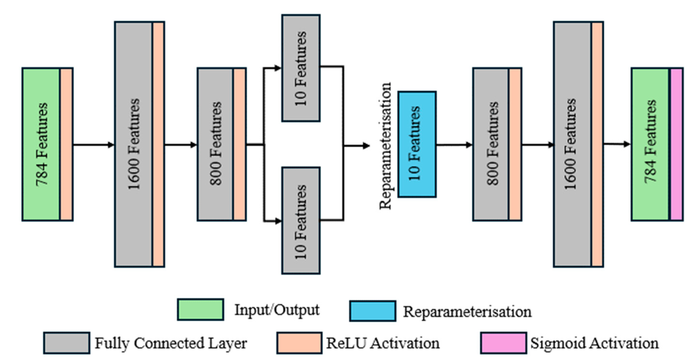
To validate the improved performance of the self-adaptive eInfoVAE, an initial case study is carried out on the MNIST handwritten digits dataset. Different VAE models are compared: standard VAE, β -VAE, untuned InfoVAE, tuned InfoVAE, eVAE, eInfoVAE using standard SBX and the newly proposed eInfoVAE using self-adaptive SBX. The models are trained on the same architecture, maintaining the same network parameters for fair comparison and performance analysed across the metrics outlined in Section 3.3. Figure 5 shows the structure of the linear network employed, resembling the structure of an autoencoder due to the bottleneck present in the middle of the network. When training VAEs, it is important to avoid entering the previously discussed mode of model collapse. To prevent model collapse, the loss function is continually monitored during training through the weights and biases interface, including the individual components of reconstruction loss, KL divergence and the MMD loss where applicable. At the end of training, the reconstruction quality is assessed both qualitatively and quantitatively, while the latent space is traversed to ensure there is no evidence of model collapse. Additionally, a comprehensive hyperparameter sweep was conducted for all base models, ensuring the hyperparameters did not initiate extreme values in the ELBO objective.
The MNIST dataset is a real-world dataset containing approximately 60,000 images of handwritten digits taken from the Modified National Institute of Standards and Technology (MNIST) database [42]. The digits vary in their construction due to the large number of handwriting styles seen in the real world, thus producing a simple yet suitably varied dataset that is perfect for training machine learning algorithms. The training dataset used in the experiments consisted of the first 50,000 images, while the evaluation dataset was composed of the final 10,000 images.
A number of network parameters appear across all seven models, these being the learning rate, number of latent dimensions, number of training epochs and the batch size of the training data. These parameters are kept constant across all the experiments to compare the models fairly and ensure the ELBO objectives and evolution strategies provide the differences in model performance. Table 1 gives the details and values of these parameters. It should be noted that, as per Section 3.3.3, to plot a meaningful latent space, the number of latent dimensions must be restricted to two. However, all other metrics were run on the ten latent dimensions model. Adam is selected as the optimiser used to update the network weights, while the number of training epochs is determined by the comparison of the evaluation and training datasets.
Across the models compared, there are a number of hyperparameters to be set. These are summarised in Table 2, where η α and η λ are the distribution indexes for α and λ , respectively. Hyperparameters were sampled randomly for the evolutionary models to allow for variation and location of the optimal solution. All distributions are random uniform distributions. The β -VAE and untuned InfoVAE models are designed to replicate experiments by the respective authors [8,9], and the parameters for the tuned InfoVAE model were determined after using the Weights and Biases sweep feature to sweep the hyperparameter space over many runs, hence locating an optimal tuning. It should also be noted that alpha is always bounded by α < 1 at all times to ensure a positive KL divergence value and model stability.

3.4.2. Experimental Setup on the Aircraft Image Dataset

To further assess the performance of the SA-eInfoVAE, it is trained on a more challenging aeronautical dataset, a set of 17,741 images of aircraft models that were sourced from the ShapeNetCore repository [43]. The dataset contains images of a wide range of aircraft models, including civil airliners, private and business jets, military fighter jets, cargo aircraft and a range of propellor aircraft, featuring both historic and modern models. The images are of 3D CAD models, taken from the default angles, i.e., front, left, back, right, top, bottom and a number of orientations of the isometric view. They are initially coloured images but converted to greyscale images, as colour does not impact geometry generation and adds an extra two channels, unnecessarily increasing the computational cost of training. Each image is square and shaped as 100 × 100 pixels, totalling 10,000 pixels per image to ensure significant amounts of detail in the dataset. The training and evaluation data are split 80–20% after a random shuffle, meaning the training dataset contains 14,195 images and the evaluation dataset contains 3549 images. The number of training epochs is once again set at 20; this is largely due to the far larger image size, resulting in a much greater computational and time cost. However, while there is scope for further training, it also provides direct comparison with the quality of the qualitative results on the MNIST dataset.
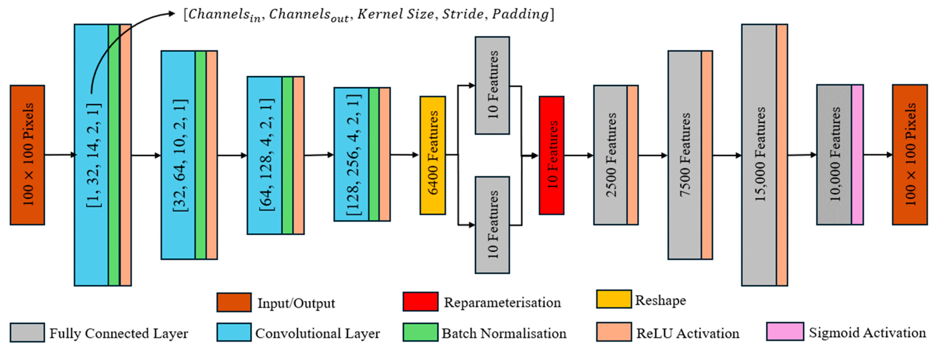
Although the network architecture outlined in Figure 5 is powerful, a new network structure was built to increase the power of the encoder. The new model architecture, detailed in Figure 6, employs convolutional layers to improve the model’s feature recognition on an increased complexity dataset. A linear decoder is still employed to ensure that the decoding distribution does not become too complex, avoiding the information preference problem. Table 3 and Table 4 detail the network parameters and hyperparameter settings and initialisations, and once again, Adam is chosen as the model optimiser.

4. Results

4.1. Validation on the MNIST Dataset

4.1.1. Loss Function and Hyperparameter Evolution

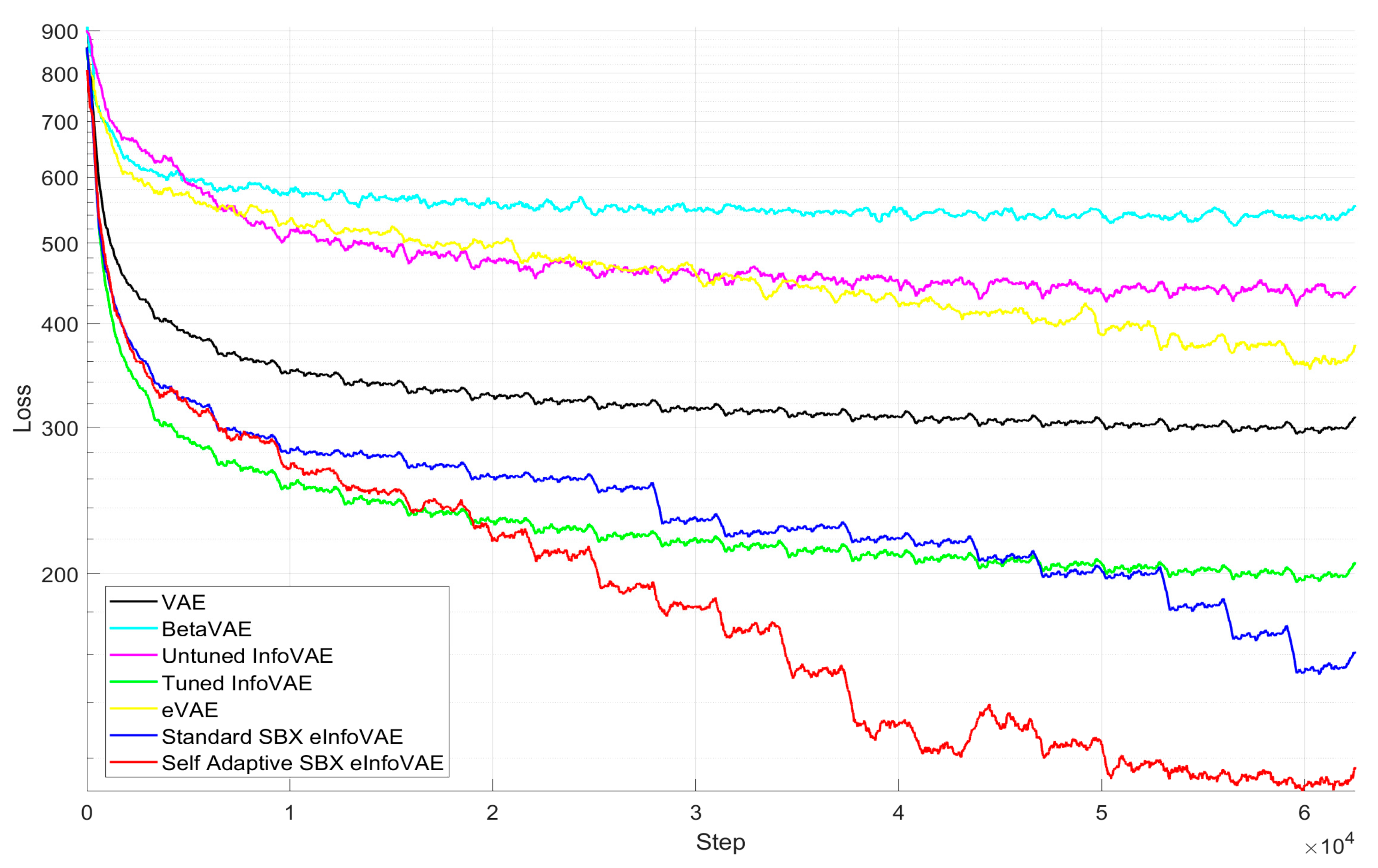
Figure 7 shows a comparison of the loss function for all five models, logged over the course of the 20 training epochs, where each step on the x -axis represents a batch of 16 images. The general trend is evident. The loss values start high and rapidly decrease as the weights of the model begin to adjust accordingly. After a short period, the model weights tend towards the optimal values and the gradient declines into a plateau, shown clearly by the standard VAE and untuned InfoVAE models. The addition of evolutionary optimisation has a clear impact on the loss function, introducing a step-like nature to the function as the hyperparameters are updated over time.
Several initial insights can be drawn from further analysis of Figure 7, the most significant of these being the levels of performance achieved by each model. SA-eInfoVAE produces the lowest loss value by some margin, with both Info evolutionary models outperforming the standard VAE and InfoVAE models. This highlights the impact a hyperparameter evolution strategy can have on loss function performance, efficiently outperforming a well-tuned model over the course of a single training run. The differing search power of the evolution strategies is shown in Figure 7, causing a significant difference in model performance. The self-adaptive SBX operation has an increased search power and precision over the standard form, moving below the tuned InfoVAE model significantly earlier. The end of training is also interesting to note, with the self-adaptive SBX model starting to converge, demonstrating improved accuracy. In contrast, the standard SBX model takes large steps in the final epochs, suggesting it has not converged to an optimal solution.
Despite being outperformed, the non-evolutionary models still provide useful insights. The fact that the untuned InfoVAE is found to be the worst performing model of the Info family highlights the importance of hyperparameter tuning. Meanwhile, the tuned InfoVAE model demonstrates the advantages of modifying the ELBO objective with hyperparameters can have, showing significantly improved performance over the standard VAE model.
In contrast, the β -VAE family of models, including eVAE, perform poorly in comparison to the Info family of models, showing the importance of designing an effective ELBO objective. Again, the evolutionary aspect of eVAE allows it to improve on the baseline set by β -VAE and beating out the untuned InfoVAE model, demonstrating the improvement an evolution strategy brings.
Figure 8 details the progression of the evolutionary models’ hyperparameters over the course of the training. There is a clear trend for α , rising toward 1 in both cases, whilst neither model displays a significant trend for λ ; however, both agree the 20–30 range is the optimal value. The trend of α in Figure 8 is not surprising upon further inspection of the ELBO objective of the InfoVAE model, detailed in Equation (4). In Equation (4), the KL divergence term is factored by 1     α ; hence, when α = 1 , the term is zero, and the KL divergence can become infinitely large without impacting the performance of the loss function. This phenomenon was noted during training, as values of α > 1 would cause large instability in the model, as the distributions diverged rapidly after this condition was met. It is for this reason that α is bounded to α < 1 , demonstrated well by the self-adaptive SBX model in Figure 8, as it plateaus just before reaching 1.
Figure 8 also demonstrates the improved search power of the self-adaptive model, producing a consistent gradient of α , while the standard model wanders significantly, changing direction numerous times up to epoch 15.

4.1.2. Generative Performance

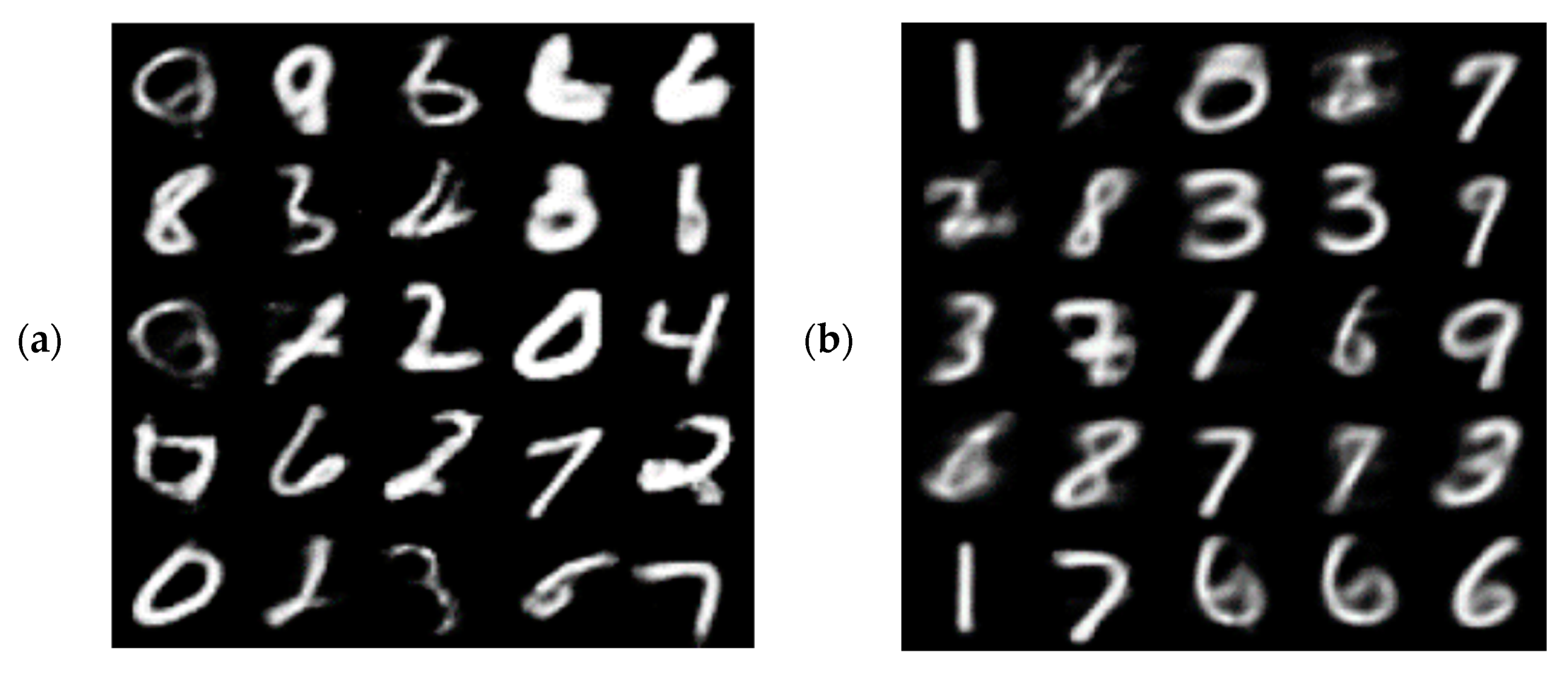
Figure 9 shows the generative performance of the models when the latent vector is sampled from the standard normal distribution; a set of ground truth images from the dataset is provided in Figure 9h for comparison. At first glance, there is clearly a range of performances, both between the models and within the digits generated by a single model.
The VAE and tuned InfoVAE (Figure 9a and Figure 9c, respectively) display the worst performance with roughly half the digits significantly distorted or incomplete. A prime example of this is the first image in row four of Figure 9a, which more closely resembles a square than a smooth zero. Despite these issues, the images generated by these models are generally sharp in the event a full digit is decipherable.
The untuned InfoVAE model, shown in Figure 9b, produces a curious result. Overall, the model generates clearly decipherable digits but with a clear fuzziness to the overall image. The untuned model has a significantly higher value of the scaling parameter λ compared to the other models, suggesting that a high value may result in improved model inference, as was the reason for introducing the parameter initially. Figure 9b does, however, suggest that the value of λ in this case is too high, and the reconstructive performance is negatively impacted by this. However, these shortcomings may be overcome by the use of pixel thresholding, a technique in which pixels below or above a given intensity have their value set to the maximal value—0 and 1, in this case [44]. Given that the MNIST dataset is binarized and, therefore, the results are greyscale images, the technique would rectify the issue here but may not be applicable on more complex natural image datasets.
The β -VAE models shown in Figure 9e,f exhibit better generative performance compared to the standard VAE and base InfoVAE models. Interestingly, the β -VAE model shows similar traits to the untuned InfoVAE model, producing generally fuzzier images but with a stronger encoding in comparison to the eVAE model, showing some significant distortion in Figure 9f.
The evolutionary Info models (shown in Figure 9d,g, respectively) outperform the previous models, with the large majority of generated samples sharp and clearly distinguishable as digits. There are still a few examples of distorted images, suggesting further model performance could potentially be extracted. However, sharp and distinguishable digits demonstrate both strong latent encodings and reconstructive performance. It is also interesting to note across Figure 9a–g that the shaper images tend to have thicker strokes, especially in comparison to Figure 9h, suggesting the model finds the thicker digits of the dataset easier to encode.

4.1.3. Reconstructive Performance

Figure 10 shows the results of the digit reconstruction process for each model, with the original input images also shown for direct comparison. Figure 10 shows that the models generally achieve far better reconstructive performance than the generative performance achieved in Figure 9. However, this is likely due to the random sampling aspect of the generative method, which gives no control over where the latent vector is sampled from, thus producing a weak generation. It is therefore evident that generating the latent vector from an input significantly increases the generative performance of the decoder.
The performance trends of Figure 10 replicate those seen in both Figure 7 and Figure 9, with the order or model performance matching that of Figure 7. The β -VAE and untuned InfoVAE models perform the worst, generating depictable but largely fuzzy images, providing further evidence for the conclusions drawn from Figure 9 and suggesting the Info model is very poorly tuned, as expected. Once again, there is a clear improvement in the tuned InfoVAE over the standard VAE model shown in Figure 10c and Figure 10a, respectively, demonstrating both the importance of hyperparameter tuning and of modifying the ELBO objective using hyperparameters to improve model performance. It is interesting to note the digits that perform particularly poorly across the range, these being the digits 2, 4 and 5. This is most evident in Figure 10a,b, where the reconstructed 5 digit is largely curved compared to the zigzag style seen in the input image. The 2 digits suffer from a lack of sharpness and general definition of the shape across the board, while the 4 digits lack finesse in their shape.
Both β -VAE models in Figure 10d,e perform relatively poorly in comparison to the InfoVAE models, producing fuzzy reconstructions and showing the importance of a good ELBO objective. The β -VAE in Figure 10d even features a distorted 8 digit; however, the eVAE model in Figure 10e significantly improves on the original, once again showing the benefits of evolutionary hyperparameter tuning.
Both Info evolutionary models, seen in Figure 10f and Figure 10g, respectively, outperform the other models, narrowly beating the tuned InfoVAE model of Figure 10c. The InfoVAE model performs well but still reproduces a slightly curved 5 digit and suffers with quality on digits 2 and 8. A qualitative comparison shows the evolutionary models produce the best reconstructive performance, demonstrating the benefits of a hyperparameter tuning evolution strategy on the model performance. However, the differences between Figure 10f,g are minimal, and so it is useful to employ a quantitative metric to further differentiate between the performance of the models. Table 5 details the result of calculating the pixel-wise mean square error between the input and the reconstructed output.
Table 5 provides further evidence for the conclusions drawn from Figure 10, agreeing with the order of performance of the models. This order is, from worst to best, β -VAE, untuned InfoVAE, eVAE, standard VAE, tuned InfoVAE, standard SBX eInfoVAE and, finally, self-adaptive SBX eInfoVAE outperforming all the other models. Table 5 can also offer new insights, showing that, on average, the self-adaptive SBX model outperforms the standard version; however, the latter does show better performance for the digits 0, 2 and 7, showing the differences are minimal. Table 5 also suggests that digits 0, 8 and 9 were reconstructed poorly, although this is less evident from the qualitative comparisons seen in Figure 10. This is potentially due to the fact that these images are still high quality in nature, i.e., sharp and clear, but the physical shape of the digit does not match that of the input as well as it should.

4.1.4. Disentanglement Performance

Table 6 shows the results of the disentanglement metric when run on the 10 latent dimension model, where a score of 100% represents a fully disentangled representation. The results give a quantitative insight into the level of encoding, acting to measure how well the approximate posterior matches the true posterior. The results follow a similar pattern as before, with both Info evolutionary models outperforming the base Info models, and the β -VAE models perform particularly poorly, even losing out to the standard VAE. It is however interesting to note the untuned InfoVAE model outperforms it’s tuned counterpart, providing further evidence to the conclusions drawn from Figure 9b that a high scaling parameter λ results in improved model inference, even when the α hyperparameter is not optimally tuned.

4.1.5. Comparison of the Latent Space

Figure 11 shows the visualised approximate prior distributions in comparison to the standard normal ground truth distribution p ( z ) . The SA-eInfoVAE model of Figure 11h shows the closest distribution to the true prior, displaying a well-rounded, slightly smaller distribution that exhibits a much sharper peak around the mean compared to the prior. The standard SBX model in Figure 11g has a more rounded peak around the mean but displays deviation, with three spikes clearly protruding. Both the VAE and untuned InfoVAE model, shown in Figure 11b and Figure 11c, respectively, underestimate the distribution significantly and produce oddly shaped mappings.
For the untuned InfoVAE model, this is in direct contrast to the previously drawn conclusions that a large scaling parameter value improves the model inference. However, there are other possible explanations for this poor latent space. It is possible the poor mapping is the result of a poorly tuned α parameter, as this hyperparameter is designed to increase the inference between X and Z , hence improving the quality of the approximate prior. However, if this value is poorly selected, the model has little reason to encourage mutual information between X and Z , resulting in the poor latent mapping seen in Figure 11c. This result suggests, along with the trends of Figure 8, that α is the dominant hyperparameter in the InfoVAE ELBO objective and has a greater impact on the model performance compared to λ . It is also interesting to note that the tuned InfoVAE model significantly overestimated the distribution, suggesting a balance of the hyperparameters is necessary for the optimal model performance.
The β -VAE models once again perform poorly, with the β -VAE model estimating an extremely narrow distribution in Figure 11e. The eVAE model displays a much more rounded distribution, much closer to that of the standard VAE model, showing the benefits of an evolution strategy. It is also interesting to note that the eVAE distribution is the only distribution to be significantly off-centre, suggesting a very poor encoding, seen in Figure 11f.
Figure 12 visualises the latent space in a different manner, by traversing across the two latent dimensions and showing the generated output at each grid position. By analysing these plots, it is possible to evaluate the quality of the latent space and map the location specific digits in the encoded latent space. This is incredibly useful for a user looking to exploit the VAE for generative modelling, allowing the user to specify the values of the latent vector to obtain a specific digit or style of digit. Unfortunately, due to the limitations of a three-dimensional world, this technique does not scale well above two or three dimensions. However, for higher dimensional spaces, the use of other dimensionality reduction algorithms such as t-SNE can be applied to map a latent space to a two-dimensional space while retaining the relationship between local variables [45]. Although not presented here, the t-SNE algorithm is useful for producing similar feature maps for higher dimensional latent spaces.
Figure 12 shows the capability of the VAE model to compress a high-dimensional space into a low-dimensional representation. The plots also visualise how the model encodes features into the latent space, perhaps shown best by the far-right column of Figure 12d. The column begins by encoding the digit 7; progressing down the column, the encoding shifts to increasingly poorly written 7s as the top stroke of the digit becomes absent. Progressing further shows the encoding progresses seamlessly into the section of digit 1s, which slowly increases in slant angle until the significantly slanted 1 digit forms the central part of the digit 2 at the bottom of the column.
Smooth encodings such as these where digits seamlessly integrate into one another suggest a high level of inference by the model. A few examples of poor encodings do occur, particularly with the eVAE model in Figure 12f, where several digits are missing from the encoding. In Figure 12a, the bottom-right corner is trying to encode both 7 and 1 digits slanted in opposite directions to each other, resulting in increasingly poor generative performance as the two digits fight over the space. Another example arises in Figure 12g along the central column encoding the digit 5; at the top, the 5s and 1s are again at conflicting angles, causing the generative performance to suffer.
Unfortunately, due to the inability to visualise 10 dimensions, Figure 12 cannot provide insight into the disentanglement performance of the model with 10 latent dimensions. However, it is assumed that, based on the quality of the encodings in Figure 12, using a representation algorithm such as t-SNE would show the digits are well encoded into the latent space with 10 dimensions. In terms of generative performance, Figure 12 shows little difference between models, with all models producing generally high-quality outputs.

4.1.6. Final Remarks on the MNIST Dataset

Throughout Section 4.1, the SA-eInfoVAE model has been comprehensively analysed and compared against previously proposed models. Analysis of the proposed model’s performance on the MNIST dataset provides valuable insight into its fundamental capabilities. The results presented show that the SA-eInfoVAE model consistently outperforms the previous models. The model has shown it is capable of successfully learning meaningful low-dimensional representations of data, a property that will be essential when applied to high-dimensional aerodynamic design problems. Further to this, the results display other important model properties, namely the fact that the model is robust and stable to train and is able to generate high-quality images. The initial testing also allows for tinkering with the evolution strategy; using a simple dataset for this provides clarity to any changes made. This validation and the resulting insights can be extrapolated with confidence to suggest that the SA-eInfoVAE model will be well suited to tackling more complex challenges in aerodynamic design optimisation, eventually leading to more efficient aerodynamic design processes.

4.2. Results on the ShapeNetCore Aircraft Image Dataset

Figure 13 displays a series of selected image inputs, deliberately selected to provide a range of views and aircraft models, along with the reconstructed images that resulted from passing the image through the trained model. It is initially clear that the SA-eInfoVAE model has enforced a high level of model performance, resulting in a generally high-quality reconstructive performance across a range of inputs in Figure 13. Images 3, 4, 6 and 7 are particularly impressive, reproducing images that, at eye level, are near identical to the model inputs.
However, some defects are also apparent, particularly with images 8 and 9, where the output is particularly grainy, producing a static-like effect in contrast to the solid shades seen in the input. This suggests these models have not been well encoded into the latent space but could also be the result of the pixel thresholding applied to the outputs, where pixel values greater than 0.85 are set to 1 (white). Image 5 also shows deformation, particularly on the wings, where the pixels appear jumbled, despite forming a relatively accurate wing shape. A comparison of images 2 and 10 provides encouraging results, showing that even small details such as engine positioning in two very similar models can be accurately differentiated by the model. On the whole, Figure 13 suggests that, on a complex dataset, such as 3D aircraft point clouds, the SA-eInfoVAE model would provide an adequate performance, able to produce high-quality reconstructed models that can be easily meshed without significant work in post-processing such as mesh repair.
Figure 14 displays a visualisation of the latent space, similar to those seen in Section 4.1.6, generated by restricting the latent dimensions to two. Figure 14 provides a different insight into the performance of the self-adaptive eInfoVAE model, suggesting a significant portion of the dataset has not been well encoded by the model. The righthand side of Figure 14 shows that the civil airline-type aircraft has been well inferred and encoded by the model, shown through the higher quality of image generation and smoother transitions between different image viewpoints. However, the left side of Figure 14 displays a different story, showing poor generative performance and an inability to distinguish the specific features of these models, highlighted best by the initial images of rows 5 and 6, simply resembling a blob of pixels. It is clear the model does not distinguish the fine details of these models, only capturing the generic shape.
There are a few possibilities for why this could be occurring. Firstly, on average, military jets are typically more varied than civil airliners, which generally all take the same form and only essentially differ in the number of engines and their locations. In contrast, military aircraft display a large number of different wing, engine, control surface and tail configurations. It is possible the model fails to learn these details as a result of insufficient occurrences in the dataset resulting in a jumbled encoding as the model attempts to encode all the different configurations in the same space.
Secondly, the nature of the dataset may also play a role in this issue. Due to the normalised size of the images, the features of the civil airliner models tend to be smaller as the viewpoint is farther from the model. Therefore, when the convolutional layers are applied over the image, due to the smaller filter size, the smaller features are picked up faster and, hence, better encoded into the latent space. For an image of a fighter jet, where the aircraft body takes up a larger proportion of the image due to the closer viewpoint and larger proportions, it would require a larger filter size to distinguish these elements as a feature. This phenomenon is particularly evident in the bottom row of Figure 14, where, as the aircraft body length increases across the row and the proportions of the image change, the encoding and image quality improve significantly. This would also explain why the “front on” images of the airliners, which have the smallest features, are so well encoded and reconstructed by the model in the top right corner of the latent space.
Despite these, Figure 14 also shows signs of good encoding, most noticeable when tracking rows 8 and 9 from left to right. In these rows, the model flows steadily from a fighter jet-type shape into an airliner-type shape, rotating through a range of views in the process. As these rows represent the middle of the latent space, this may also suggest that, with a finer grid size, an increased number of image viewpoints would be seen in the latent encoding.

5. Conclusions and Discussion

This study has introduced a new self-adaptive evolutionary info variational autoencoder (SA-eInfoVAE) model, building on the work of both the InfoVAE and eVAE models to combine the approaches of improving model performance. Additionally, the evolution strategy used has also been modified to the self-adaptive simulated binary crossover operation, improving both the search power and precision of the evolution strategy. The implementation of this model, including network architecture, training loops and comparative metrics, was detailed in Section 3.
The new model was first validated on the MNIST dataset against six state-of-the-art models under the same training conditions. The results from this comparative testing proved that the SA-eInfoVAE model outperformed all six models across a range of metrics, displaying improved generative, reconstructive, disentanglement and latent encoding performance. The dynamic tuning allowed the model to find a better hyperparameter pair over the course of just one training run, outperforming a tuned InfoVAE model that had been manually tuned over the course of many runs, saving a significant amount of training time. This was largely due to the improved search power and precision of the self-adaptive simulated binary crossover operator in comparison to the standard version implemented in eVAE. These results show the SA-eInfoVAE model is capable of slashing training times and hence significantly reducing the computational cost to build a well-trained model, which will scale effectively on large and complex datasets.
The results of Section 4 also provided insight into potential issues faced by the SA-eInfoVAE model, largely stemming from the form of the InfoVAE ELBO objective. Figure 8 demonstrates the tendency of the evolution strategy to push α towards 1, hence eliminating the KL divergence term at α = 1 or allowing the inferred posterior distribution to diverge from the true distribution when α > 1 . Whilst this issue can be avoided by bounding α < 1 , it shows potential instability in the ELBO objective, particularly when the evolution strategy is aiming to push the limits of its performance. It is therefore suggested that future work should aim to mitigate the KL vanishing effect at α = 1 , potentially by utilising different ELBO objectives or even designing a new objective entirely. Whilst the results suggested the self-adaptive binary crossover operator to be sufficiently powerful and precise, further work could also include a comparison of evolution strategies to determine the best strategy for hyperparameter tuning. However, it should be noted that increasing the complexity of the evolution strategy is likely to increase the computational cost, negating one of the main benefits of the model, and so, future evolution strategies should be computationally minimal whilst improving the search capabilities. Whilst the performance on the MNIST dataset was impressive, many useful applications of the VAE involve far more complex datasets. The assessment of the SA-eInfoVAE model on a dataset of aircraft images produced mixed results, performing well in reconstructive tasks but displaying evidence of weak encoding for a significant proportion of the models in the latent space. In a workflow similar to that of Figure 1, it was hoped that the implementation of the SA-eInfoVAE model would provide an adequate geometry generation performance and, in comparison to other VAE models, significantly reduce both the training time and computational cost based on the conclusions drawn from the results of this study.

6. Future Work

Future work should investigate different network architectures; further validation on benchmarking datasets such as CIFAR-10 [46], CelebA [28] and chairs [29] and normalisation strategies. It is also suggested that, should the same or similar datasets be used, that the data be split into military and civil applications. This would allow different network architectures to be implemented to ensure detailed representations could be learnt instead of forcing the model to balance the two data types, diminishing the model performance. It is also necessary to bring quantitative and further qualitative analyses to the ShapeNet dataset to further validate the proposed models’ abilities on a more complex dataset. However, in the context of aerodynamic optimisation, future work should inevitably focus on extending this work initially to the 2D aerofoil domain for synthesis and analysis. After comprehensive evaluation at this level, especially against AirfoilGAN, this work should also be extended to the 3D domain, using point cloud data to synthesise novel aerodynamic aircraft designs. It is hopeful that the proposed model would be able to be combined with CFD data to predict the performance of newly synthesised geometries.

Author Contributions

Conceptualisation, T.A.E. and Y.Z.; methodology, T.A.E.; software, T.A.E.; validation, T.A.E.; formal analysis, T.A.E.; data curation, T.A.E.; writing—original draft preparation, T.A.E.; writing—review and editing, T.A.E. and Y.Z.; supervision, Y.Z. All authors have read and agreed to the published version of the manuscript.

Funding

This research received no external funding.

Data Availability Statement

Data and the Python program used in this study can be found from the GitHub repository: https://github.com/tobyemm7/Self-Adaptive-Evolutionary-Info-Variational-Autoencoder.git, accessed on 20 June 2024. The aircraft image dataset from ShapeNetCore is available to download at https://shapenet.org/ (accessed on 13 May 2024).

Conflicts of Interest

The authors declare no conflicts of interest.

References

  1. Li, J.; Xiasong, D.; Martins, J.R.R.A. Machine Learning in Aerodynamic Shape Optmisation. Prog. Aeronaut. Sci. 2022, 134, 100849. [Google Scholar] [CrossRef]
  2. Kingma, D.P.; Welling, M. Auto-Encoding Variational Bayes. arXiv 2013, arXiv:13.12.6114. [Google Scholar] [CrossRef]
  3. Rezende, D.J.; Mohammed, S.; Wierstra, D. Stochastic Backpropagation and Approximate Inference in Deep Generative Models. In Proceeding of the 31st International Conference on Machine Learning, Beijing, China, 21–26 June 2014. [Google Scholar]
  4. Burda, Y.; Grosse, R.; Salakhutdinov, R. Importance Weighted Autoencoders. arXiv 2015, arXiv:1509.00519. [Google Scholar] [CrossRef]
  5. Saha, S.; Minku, L.; Yao, X.; Sendhoff, B.; Menzel, S. Exploiting 3D variational autoencoders for interactive design. Proc. Des. Soc. 2022, 2, 1747–1756. [Google Scholar] [CrossRef]
  6. Rios, T.; Stein, B.V.; Wollstadt, P.; Back, T.; Sendhoff, B.; Menzel, S. Exploiting Local Geometric Features on Vehicle Design Optimization with 3D Point Cloud Autoencoders. In Proceeding of the 2021 IEEE Congress on Evolutionary Computation (CEC), Krakow, Poland, 28 June–1 July 2021. [Google Scholar] [CrossRef]
  7. Mrosek, M.; Othmer, C.; Radepsiel, R. Variational Autoencoders for Model Order Reduction in Vehicle Aerodynamics. In Proceeding of the AIAA Aviation Forum, Virtual, 2–6 August 2021. [Google Scholar] [CrossRef]
  8. Higgins, I.; Matthey, L.; Pal, A.; Burgess, C.; Glorot, X.; Botvnick, M.; Mohamed, S.; Lerchner, A. Beta-VAE: Learning Basic Visual Concepts with a Constrained Variational Framework. In Proceeding of the 5th International Conference on Learning Representations, Toulon, France, 24–26 April 2017. [Google Scholar]
  9. Zhao, S.; Song, J.; Ermon, S. InfoVAE: Balancing Learning and Inference in a Variational Autoencoders. In Proceedings of the 31st AAAI Conference on Artificial Intelligence, Honolulu, HI, USA, 27 January–1 February 2019. [Google Scholar] [CrossRef]
  10. Shao, H.; Yao, S.; Sun, D.; Zhang, A.; Liu, S.; Liu, D.; Wang, J.; Abdelzaher, T. ControlVAE: Controllable Variational Autoencoder. In Proceedings of the 37th International Conference on Machine Learning, Virtual, 13–18 July 2020. [Google Scholar]
  11. Bond-Taylor, S.; Leach, A.; Long, Y.; Willcocks, C.G. Deep Generative Modelling: A Comparative Review of VAEs, GANs, Normalizing Flows, Energy-Based and Autoregressive Models. IEEE Trans. Pattern Anal. Mach. Intell. 2022, 44, 7327–7347. [Google Scholar] [CrossRef]
  12. Seong, J.Y.; Ji, S.; Choi, D.; Lee, S.; Lee, S. Optimizing Generative Adversarial Network (GAN) Models for Non-Pneumatic Tire Design. Appl. Sci. 2023, 13, 10664. [Google Scholar] [CrossRef]
  13. Andriyanov, N.A.; Vasiliev, K.K.; Dementiev, V.E.; Belyanchikov, A.V. Restoration of Spatially Inhomogeneous Images Based on a Doubly Stochastic Model. Optoelectron. Instrument. Proc. 2022, 58, 465–471. [Google Scholar] [CrossRef]
  14. Bamford, T.; Keane, A.; Toal, D. SDF-GAN: Aerofoil Shape Parameterisation via an Adversarial Auto-Encoder. In Proceedings of the AIAA Aviation Forum and Ascend 2024, Las Vegas, NV, USA, 29 July–2 August 2024. [Google Scholar] [CrossRef]
  15. Du, X.; He, P.; Martins, J.R.R.A. A B-Spline-based Generative Adversarial Network Model for Fast Interactive Airfoil Aerodynamic Optimization. In Proceedings of the AIAA Scitech 2020 Forum, Orlando, FL, USA, 6–10 January 2020. [Google Scholar] [CrossRef]
  16. Chen, W.; Chiu, K.; Fuge, M. Aerodynamic Design Optimization and Shape Exploration using Generative Adversarial Networks. In Proceedings of the AIAA Scitech 2019 Forum, San Diego, CA, USA, 7–11 January 2019. [Google Scholar] [CrossRef]
  17. Yu, X.; Zhang, X.; Cao, Y.; Xia, M. VAEGAN: A Collaborative Filtering Framework based on Adversarial Variational Autoencoders. In Proceedings of the 28th International Conference on Artificial Intelligence, Macao, China, 10–16 August 2019. [Google Scholar]
  18. Wang, Y.; Shimada, K.; Farimani, A.B. Airfoil GAN: Encoding and synthesizing airfoils for aerodynamic shape optimization. J. Comput. Des. Eng. 2023, 10, 1350–1362. [Google Scholar] [CrossRef]
  19. Blei, D.M.; Kucukelbir, A.; McAuliffe, J.D. Variational Inference: A Review for Statisticians. J. Am. Stat. Assoc. 2017, 112, 859–877. [Google Scholar] [CrossRef]
  20. Shlens, J. Notes on Kullback-Leibler Divergence and Likelihood Theory. arXiv 2014, arXiv:1404.2000. [Google Scholar] [CrossRef]
  21. Doersch, C. Tutorial on Variational Autoencoders. arXiv 2016, arXiv:1606.05908. [Google Scholar]
  22. Tomczak, J.M.; Welling, M. VAE with VampPrior. In Proceedings of the International Conference on Artificial Intelligence and Statistics (AISTATS), Playa Blanca, Spain, 9–11 April 2018. [Google Scholar]
  23. Van Den Oord, A.; Kalchbrenner, N.; Kavukcuoglu, K. Pixel Recurrent Neural Networks. In Proceedings of the 33rd International Conference on Machine Learning, New York, NY, USA, 19–24 June 2016. [Google Scholar]
  24. Gulrajani, I.; Kumar, K.; Ahmed, F.; Taiga, A.A.; Visin, F.; Vazquez, D.; Courville, A. PixelVAE: A Latent Variable Model for Natural Images. arXiv 2016, arXiv:1611.05013. [Google Scholar] [CrossRef]
  25. Razavi, A.; Van Den Oord, A.; Poole, B.; Vinyals, O. Preventing Posterior Collapse with delta-VAEs. arXiv 2019, arXiv:1901.03416. [Google Scholar] [CrossRef]
  26. Wu, Z.; Cao, L.; Qi, L. eVAE: Evolutionary Variational Autoencoder. IEEE Trans. Neural Netw. Learn. Syst. 2024, accepted. [Google Scholar] [CrossRef] [PubMed]
  27. Fu, H.; Li, C. Cyclical Annealing Schedule: A simple Approach to Mitigating KL Vanishing. In Proceedings of the Annual Conference of the North American Chapter of the Association for Computational Linguistics, Minneapolis, MN, USA, 2–7 June 2019. [Google Scholar]
  28. Liu, Z.; Luo, P.; Wang, X.; Tang, X. Deep Learning Face Attributes in the Wild. In Proceedings of the IEEE International Conference on Computer Vision (ICCV), Santiago, Chile, 7–13 December 2015; pp. 3730–3738. [Google Scholar]
  29. Aubry, M.; Maturana, D.; Efros, A.A.; Russell, B.C.; Sivic, J. Seeing 3D Chairs: Exemplar Part-based 2D-3D Alignment using a Large Dataset of CAD Models. In Proceedings of the IEEE Conference on Computer Vision and Pattern Recognition (CVPR), Columbus, OH, USA, 23–28 June 2014; pp. 3762–3769. [Google Scholar]
  30. Paysan, P.; Knothe, R.; Amberg, B.; Romdhani, S.; Vetter, T. A 3D Face Model for Pose and Illumination Invariant Face Recognition. In Proceedings of the 2009 Sixth IEEE International Conference on Advanced Video and Signal Based Surveillance, Genova, Italy, 2–4 September 2009; pp. 296–301. [Google Scholar] [CrossRef]
  31. Chen, X.; Duan, Y.; Houthooft, R.; Schulman, J.; Sutskever, I.; Abbeel, P. InfoGAN: Interpretable Representation Learning by Information Maximizing Generative Adversarial Nets. In Proceedings of the Advances in Neural Information Processing Systems 29 (NIPS), Barcelona, Spain, 5–10 December 2016. [Google Scholar]
  32. Kulkarni, T.D.; Whitney, W.F.; Kohli, P.; Tenenbaum, J. Deep Convolutional Inverse Graphics Network. In Proceedings of the Advances in Neural Information Processing Systems 28 (NIPS), Montreal, QC, Canada, 7–12 December 2015. [Google Scholar]
  33. Alemi, A.; Poole, B.; Fischer, I.; Dillon, J.; Saurous, R.A.; Murphy, K. Fixing a Broken ELBO. In Proceedings of the 35th International Conference on Machnine Learning, Stockholm, Sweden, 10–15 July 2018. [Google Scholar]
  34. Gretton, A.; Borgwardt, K.M.; Rasch, J.M.; Schölkopf, B.; Smola, A. A Kernel Two-Sample Test. J. Mach. Learn. Res. 2012, 13, 723–773. [Google Scholar]
  35. Deb, K.; Agrawal, R.B. Simulated Binary Crossoer for Continuous Search Space. Complex Syst. 1995, 9, 115–148. [Google Scholar]
  36. Chacón, J.; Segura, C. Analysis and Enhancement of Simulated Binary Crossover. In Proceedings of the 2018 IEEE Congress on Evolutionary Computation (CEC), Rio de Janeiro, Brazil, 8–13 July 2018. [Google Scholar] [CrossRef]
  37. Deb, K.; Sindhiya, K.; Okabe, T. Self-Adaptie Simulated Binary Crossover for Real-Parameter Optimization. In Proceedings of the 9th Annual Conference on Genetic and Evolutionary Computation, London, UK, 7 July 2007. [Google Scholar]
  38. NVIDIA T4 Tensor Core GPU. Available online: https://www.nvidia.com/en-gb/data-center/tesla-t4/ (accessed on 10 April 2024).
  39. Fadel, S.; Ghoniemy, S.; Abdallah, M.; Abu Sorra, H.; Ashour, A.; Ansary, A. Investigating the Effect of Different Kernal Functions on the Performance of SVM for Recognizing Arabic Characters. Int. J. Adv. Comput. Sci. Appl. 2016, 7, 446–450. [Google Scholar]
  40. What is W&B? Available online: https://docs.wandb.ai/guides (accessed on 24 January 2024).
  41. Węglarczyk, S. Kernel Density Estimation and its Application. ITM Web Conf. 2018, 23, 00037. [Google Scholar] [CrossRef]
  42. Rani, E.G.; Sakthimohan, M.; Abhigna, R.G.; Selvalakshmi, D.; Keerthi, T.; Raja Sekar, R. MNIST Handwritten Digit Recognition using Machine Learning. In Proceedings of the 2022 2nd International Conference on Advance Computing and Innovative Technologies in Engineering (ICACITE), Greater Nodia, India, 28–29 April 2022. [Google Scholar] [CrossRef]
  43. Chang, A.X.; Funkhouser, T.; Guibas, L.; Hanrahm, P.; Huang, Q.; Li, Z.; Savarese, S.; Savva, M.; Song, S.; Su, H.; et al. ShapeNet: An Information-Rich 3D Model Repository. arXiv 2015, arXiv:1512.03012. [Google Scholar]
  44. Wellner, P.D. Adaptive Thresholding for the Digital Desk; EuroPARC Technical Report EPC-93-110; Xerox: Norwalk, CT, USA, 1993. [Google Scholar]
  45. Van Der Maaten, L.; Hinton, G. Visualizing Data using t-SNE. J. Mach. Learn. Res. 2008, 9, 2579–2605. [Google Scholar]
  46. The CIFAR-10 Dataset. Available online: https://www.cs.toronto.edu/~kriz/cifar.html (accessed on 3 August 2024).
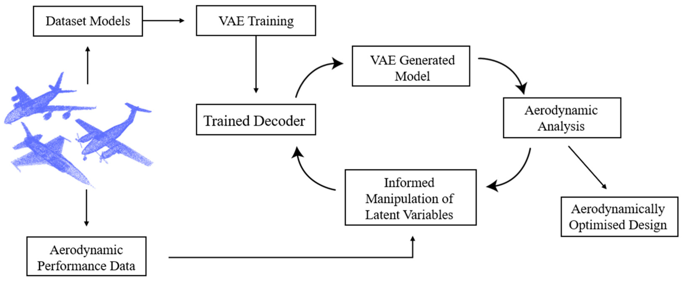
Figure 1. Workflow for automated aerodynamic design optimisation using a variational autoencoder (VAE).
Computers 13 00214 g001
Figure 2. Workflow representation of the variational autoencoder (VAE) model detailing the process of the re-parameterisation trick. The result of this is z * , computed by the workflow and designated a star to show it is representative of—not a true member of the distribution q ϕ ( z ) .
Computers 13 00214 g002
Figure 3. Workflow detailing the inner–outer training loop used in the eVAE model. The result of the cycle is β * , representing the best hyperparameter solution of the chromosome population, selected as the start of the next cycle. The red and blue distributions provide an intuitive representation of the crossover operation for distributions.
Computers 13 00214 g003
Figure 4. Workflow of the proposed self-adaptive evolutionary info variational autoencoder model. Similarly to the eVAE model, α * and λ * represent the strongest hyperparameter pair of the population and are selected to be the starting point of the next cycle. Again, the distribution in the bottom right depicts the variational crossover operation for distributions.
Computers 13 00214 g004
Figure 5. Structure of the neural network used for model comparison on the MNIST dataset.
Computers 13 00214 g005
Figure 6. Structure of the neural network used for the ShapeNetCore aircraft image dataset.
Computers 13 00214 g006
Figure 7. Comparison of the ELBO objective loss function values over a period of 20 training epochs.
Computers 13 00214 g007
Figure 8. Evolution of the α and λ hyperparameters over the course of the training run.
Computers 13 00214 g008
Figure 9. Generated image samples from (a) VAE, (b) untuned InfoVAE, (c) tuned InfoVAE, (d) standard SBX eInfoVAE, (e) β -VAE, (f) eVAE and (g) SA-eInfoVAE, and (h) ground truth images from the MNIST dataset.
Computers 13 00214 g009aComputers 13 00214 g009b
Figure 10. Comparison of the original input images and reconstructions from (a) VAE, (b) untuned InfoVAE, (c) tuned InfoVAE, (d) β -VAE, (e) eVAE, (f) standard SBX eInfoVAE and (g) SA-eInfoVAE.
Computers 13 00214 g010
Figure 11. Comparison of the visualised approximate prior distributions of the seven models with the ground truth prior.
Computers 13 00214 g011
Figure 12. Comparisons of the latent traversals of (a) VAE, (b) untuned InfoVAE, (c) tuned InfoVAE, (d) standard SBX eInfoVAE, (e) β -VAE, (f) eVAE and (g) self-adaptive SBX eInfoVAE.
Computers 13 00214 g012aComputers 13 00214 g012b
Figure 13. Comparison of the original input images and the reconstructions form the SA-eInfoVAE model on the ShapeNetCore aircraft image dataset.
Computers 13 00214 g013
Figure 14. Visualisation of the latent space for the SA-eInfoVAE model on the ShapeNetCore aircraft image dataset.
Computers 13 00214 g014
Table 1. Network parameters for experiments on the MNIST dataset.
Network ParameterLearning RateBatch SizeLatent DimensionsTraining Epochs
Value0.000351610 & 220
Table 2. Hyperparameters used for the seven models.
Hyperparameter
Model α λ β Crossover RateMutation Rate η α η λ
VAE-------
β -VAE--4----
Untuned InfoVAE01000-----
Tuned InfoVAE0.7100-----
eVAE-- β [ 3 ,   5 ] 0.30.2--
Standard SBX eInfoVAE α   [ 0.4 , 0.4 ] (Initially) λ   [ 25 , 150 ] (Initially)-0.30.283
Self-Adaptive SBX eInfoVAE α   [ 0.4 , 0.4 ] (Initially) λ   [ 25 , 150 ] (Initially)-0.30.28 (Initially)3 (Initially)
Table 3. Network parameters for the ShapeNetCore aircraft image dataset.
Network ParameterLearning RateBatch SizeLatent DimensionsTraining Epochs
Value0.000351610 & 220
Table 4. Hyperparameter settings and initialisation for the SA-eInfoVAE model on the ShapeNetCore aircraft image dataset.
ParametersInitialisations
Crossover RateMutation Rate α λ η α η λ
0.30.2 α     [ 0.4 ,   0.4 ] λ     [ 50 ,   200 ] 83
Table 5. Quantitative measures of the reconstructive performance of the compared models.
Digit Mean-Square Error (×10−1)
Model0123456789Average
VAE0.1330.0320.1590.1270.2310.3890.1160.1310.1540.1470.162
Untuned InfoVAE0.1930.0770.4540.2380.2450.4260.2860.1470.2540.3220.264
Tuned InfoVAE0.1160.0460.1630.1250.1180.2870.0940.0650.1230.1190.126
β -VAE0.2130.1170.4060.3080.2910.5280.2180.1730.2240.3720.285
eVAE0.1870.0870.2520.2670.1630.4260.1210.1600.2410.2600.216
Standard SBX
eInfoVAE
0.0890.0320.1220.1000.0800.1840.0660.0580.1200.1020.095
Self-Adaptive
SBX eInfoVAE
0.0900.0220.1300.0840.0690.1730.0450.0630.1080.0790.086
Table 6. Comparison of disentanglement metric scores across the seven models.
ModelVAEUntuned InfoVAETuned InfoVAE β -VAEeVAEStandard SBX
eInfoVAE
Self-Adaptive SBX
eInfoVAE
Disentanglement Performance/%85.490.890.345.757.191.196.6
Disclaimer/Publisher’s Note: The statements, opinions and data contained in all publications are solely those of the individual author(s) and contributor(s) and not of MDPI and/or the editor(s). MDPI and/or the editor(s) disclaim responsibility for any injury to people or property resulting from any ideas, methods, instructions or products referred to in the content.