Abstract
Predicting the future trajectories of multiple interacting pedestrians within a scene has increasingly gained importance in various fields, e.g., autonomous driving, human–robot interaction, and so on. The complexity of this problem is heightened due to the social dynamics among different pedestrians and their heterogeneous implicit preferences. In this paper, we present Information Maximizing Spatial-Temporal Graph Convolutional Attention Network (InfoSTGCAN), which takes into account both pedestrian interactions and heterogeneous behavior choice modeling. To effectively capture the complex interactions among pedestrians, we integrate spatial-temporal graph convolution and spatial-temporal graph attention. For grasping the heterogeneity in pedestrians’ behavior choices, our model goes a step further by learning to predict an individual-level latent code for each pedestrian. Each latent code represents a distinct pattern of movement choice. Finally, based on the observed historical trajectory and the learned latent code, the proposed method is trained to cover the ground-truth future trajectory of this pedestrian with a bi-variate Gaussian distribution. We evaluate the proposed method through a comprehensive list of experiments and demonstrate that our method outperforms all baseline methods on the commonly used metrics, Average Displacement Error and Final Displacement Error. Notably, visualizations of the generated trajectories reveal our method’s capacity to handle different scenarios.
1. Introduction
It is important to accurately predict pedestrian trajectories [1,2,3]. For example, in situations like crosswalks and crowded public areas, accurately predicting pedestrian trajectories can improve safety and prevent potential accidents [4,5,6,7,8].
In monitoring systems, predicting pedestrian trajectories is pivotal in facilitating the detection of anomalous behaviors [9,10,11]. Additionally, it can help optimize the planning of transportation systems with better insights into pedestrian flow and behavior modeling [12,13,14,15,16].
Forecasting the trajectory of a pedestrian still remains a significant challenge, primarily for two reasons: (1) the complexity of interactions among pedestrians in a given environment and (2) the heterogeneity in individual behavioral preferences. Regarding the first reason, there are multiple factors influencing a pedestrian’s trajectory, e.g., static obstacles like trees and roads and dynamic components including vehicles and other pedestrians. As reported by [17], up to 70% of pedestrians in a crowd move in groups, such as families or friends walking together. Such interactions are mainly driven by “social interactions” [18,19]. Regarding the second reason that this remains challenging, different individuals usually display varied behaviors under similar circumstances [20], which makes it complicated to establish a universal behavioral model that fully represents the entire population [21,22,23]. For instance, pedestrians of different ages may have distinct walking preferences [24]. Additionally, these walking preferences might further change significantly depending on whether individuals are walking alone or within a group [25]. The heterogeneity in behaviors across agents substantially influences their actions across various observational contexts [26].
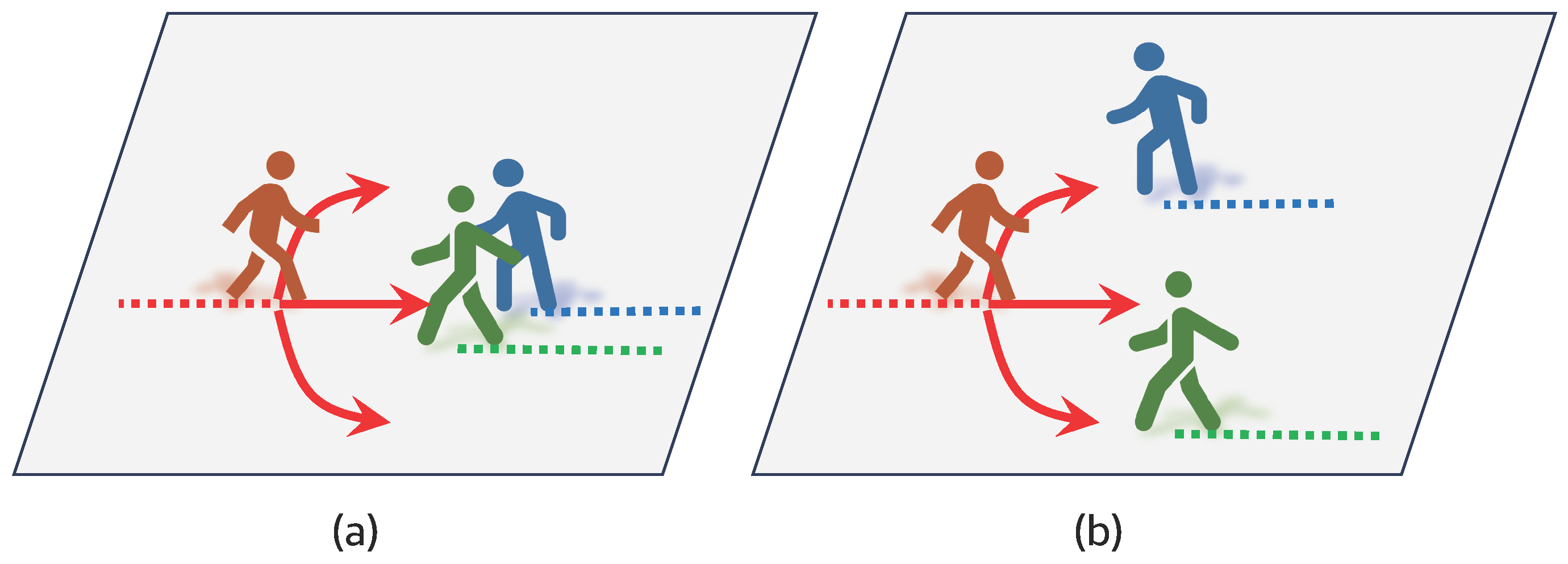
Figure 1 illustrates scenarios corresponding to the mentioned reasons, where Figure 1a shows how different pedestrians might favor different trajectories, and Figure 1b highlights the interactions of surrounding pedestrians on an individual’s decisions. Nevertheless, in the majority of the prior research, emphasis has been placed on the second aspect, i.e., how to model pedestrian interactions. One of the most classical approaches is called the “social force model” [18,19], which leverages forces such as attractive and repulsive forces to elucidate pedestrian behavior mechanisms in general.
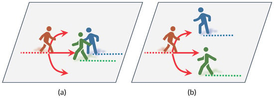
Figure 1.
(a) When an individual (in red) encounters a pair of pedestrians walking together, the reaction can vary from person to person. Some might prefer navigating to the left, while others might prefer going to the right. (b) In a scenario where a pedestrian encounters two pedestrians walking separately, the only feasible route is the middle path. For the individual (in red), choosing to go left or right might lead to a potential collision. As a result, social interactions among different pedestrians can significantly influence one’s decisions, given that individuals typically seek to avoid potential collisions with others.
Driven by the recent successes of deep learning techniques, there is a growing interest among researchers in developing deep learning-based methods to model the social interactions between pedestrians, incorporating the social attributes inherent in pedestrian movements. Social LSTM [27] is a deep learning-based method, which predicts pedestrians’ trajectories using recurrent neural networks. Subsequent research is developed based on such methodology, e.g., Peek Into The Future (PITF) [28] and State-Refinement LSTM (SR-LSTM) [29]. Another interesting direction is to use the Generative Adversarial framework [23,30,31,32,33], e.g., Social GAN [34] and Sophie [35].
Despite the existing body of research, there remains limited exploration into modeling pedestrian social interactions and heterogeneous individual behaviors simultaneously. To address the aforementioned problems, we propose InfoSTGCAN in this paper. Within this framework, we represent pedestrians’ trajectories through a spatial-temporal graph, integrating the spatial-temporal convolution and spatial-temporal attention mechanisms. Meanwhile, the behavior pattern of each pedestrian is modeled as a latent distribution based on the observed trajectory. Intuitively speaking, pedestrians with distinct latent codes have different styles of trajectories. As such, our approach not only improves predictive accuracy but also provides insights into the varied behavioral patterns exhibited by individuals.
1.1. Literature Review
1.1.1. Pedestrian Trajectory Prediction
In this section, we review the existing research focusing on the task of pedestrian trajectory prediction, which is the most related field to this paper. Generally, most pedestrian trajectory prediction methods can be typically categorized into two primary types: physics-based models and deep learning-based models.
Physics-based models One classical approach to tackle the challenge of pedestrian trajectory prediction is to utilize physics-based models. The physics-based models are usually characterized by some basic rules or generic functions, taking into account both physical constraints and pedestrians’ social or psychological factors [2,36,37,38,39,40]. One well-known physics-based model is the “cellular automaton model” [41,42]. The cellular automaton model is a discrete model, which is based on the discrete motions of pedestrians traversing a grid of cells, and it is assumed that each cell is in a finite number of states.
The second type of physics-based models is called the “social force model” [18]. The social force model is a microscopic continuous model, which studies the motions of pedestrians by some social forces, such as the destination choice and the need to avoid collisions with other pedestrians. Basically, the original social force model assumes that most of scenarios encountered by pedestrians are standard, such that behavioral strategies acquired through experience can be utilized.
Later, ref. [19] introduced “Nomad”, a generalized version of the social force model, which incorporates behavioral rules, and continuous route choice. This activity-based approach allows pedestrians to adapt their movements based on different traffic conditions, e.g., distance to a destination. In [36], the authors provided a comprehensive review of crowd motion simulation models, explaining their characteristics, applicability, and the underlying crowd movement phenomena. Interested in pedestrian behaviors at signalized crosswalks, ref. [43] adapted the social force model and calibrated its parameters using maximum likelihood estimation.
Another type of physics-based model is represented by the category of “velocity-based models”, which have been widely used in the game industry and robots [44,45,46,47]. Technically speaking, velocity-based models rely on differential equations, and their associated speed functions depend on the relative positions of the neighboring pedestrians and obstacles. For example, the reciprocal velocity obstacle model [45] is able to navigate multiple agents in real time and generates safe and oscillation-free motions. In [48], the authors proposed the optimal reciprocal collision avoidance (ORCA) model, which can provide local collision-free motions for a large number of agents within a time interval.
Deep learning-based trajectory prediction Inspired by the success of deep learning models [22,49,50,51,52,53], numerous research studies have focused on utilizing deep learning models for the task of pedestrian trajectory prediction. Social long short-term memory (Social LSTM) [27] is one of them. The Social LSTM model employs a type of recurrent network to learn the sequential movement of each pedestrian. To predict the trajectory afterwards, the “social pooling” mechanism is utilized to aggregate the output of the RNNs. Specifically, the model pools the neighbor hidden states of a pedestrian within a distance threshold. Later, based on LSTMs and Generative Adversarial Networks [30], Social GAN [34] was proposed. Social GAN designed a novel pooling mechanism that calculates interactions according to the relative distances among pedestrians.
Subsequent works have built upon Social LSTM and Social GAN [28,29,35,54]. For example, State-Refinement LSTM (SR-LSTM) [29] proposed a new pooling mechanism, which leverages the intentions of neighboring pedestrians. This approach iteratively refines the states of all pedestrians using a mechanism known as “social-aware information selection”. Peek Into The Future (PITF) [28] incorporates visual features and proposes modules that take pedestrian–scene interactions into consideration. The Sophie framework [35] is an LSTM-based generative adversarial network. It utilizes convolutional neural networks (CNNs) to extract scene features, followed by a dual attention mechanism. Subsequently, Sophie combines the attention outputs with the scene features.
Given that graph structures are able to explicitly represent the interactions of pedestrians, there has been a growing research interest in graph-based approaches [55,56]. Graph attention networks (GATs) [55] leverage the architecture of Bicycle-GAN and capture the pedestrian interactions with the help of the graph attention mechanism [55]. Recursive Social Behavior Graphs [56] utilize graph convolution networks, combined with additional social information from expert sociologists.
To directly utilize spatial and temporal information together, ref. [57] proposed the Social Spatial-Temporal Graph Convolutional Neural Network (Social-STGCNN). Social-STGCNN models pedestrian trajectories as a spatial-temporal graph, where the spatial edges represent social interactions between pedestrians, weighted by their relative distances. However, the graph kernel function in Social-STGCNN is still based on some predefined rules, e.g., pedestrians with shorter distances have higher weights. By incorporating the spatial-temporal attention mechanism, we are able to move beyond such “predefined rules”. Our proposed model learns to assign varying levels of importances to different neighbor nodes based on their features, while also taking the predefined rules into consideration.
In summary, while most previous works focus on modeling pedestrian interactions, the future trajectory of a pedestrian is usually uncertain and different pedestrians may exhibit distinct preferences regarding their behaviors. Therefore, it is not only crucial to model pedestrian interactions, but also imperative to explicitly quantify the inherent heterogeneity present within pedestrian trajectories. To bridge this gap, we introduce the InfoSTGCAN framework in this study. The proposed framework encapsulates pedestrian trajectories within a spatial-temporal graph, leveraging both convolutional and attention mechanisms across spatial and temporal dimensions. Furthermore, we model the behavioral patterns of each pedestrian as a latent distribution derived from their trajectories. This approach intuitively assigns unique latent codes to pedestrians, corresponding with distinct trajectory styles. Figure 1 illustrates such concept and Table 1 summarizes the differences between the proposed framework with the previous methods.

Table 1.
Existing research on pedestrian trajectory prediction.
1.1.2. Graph Neural Networks
Graph neural networks (GNNs) are well-suited for processing non-Euclidean data [59,60,61]. There are several kinds of GNNs [62,63,64,65,66,67,68,69]: Recurrent graph neural networks, convolutional graph neural networks, graph attention networks and so on.
Convolutional graph neural networks Basically, there are two major types of convolutional graph neural networks: spectral-based approaches and spatial-based approaches. Spectral-based approaches develop convolution operations based on the graph Fourier transform, e.g., GCNs [60],and ChebNet [62]. Spatial-based approaches perform convolution directly on the edges, making them suitable for asymmetric adjacency matrices, e.g., GraphSage [63] and DGCNN [64]. To deal with the spatial-temporal data, ST-GCN [70] expands the spatial GCN into a spatial-temporal version for the task of skeleton-based action recognition, incorporating information from a localized spatial-temporal context.
Graph attention networks Attention has been widely used in a series of tasks, e.g., machine translation [71], entity resolution [72] and so on. Proposed by [73], graph attention networks bring attention mechanisms to graph neural networks, which calculate the relative weights between two connected nodes by the attention scores. Later, [74] proposed GeniePath, which controls the flow of information by some LSTM-style gating mechanisms.
1.2. Contributions
Specifically, the main contributions of this paper are highlighted as follows:
- We formulate the task of pedestrian trajectory prediction as a spatial-temporal graph and propose a novel trajectory prediction model, InfoSTGCAN. This model takes both pedestrian interactions and heterogeneous behavior choice modeling into consideration. Through a comprehensive list of experiments, we demonstrate the superiority of InfoSTGCAN in comparison to existing baseline methods.
- Our proposed method integrates spatial-temporal graph convolution and spatial-temporal graph attention. This fusion enables our method to more effectively model pedestrian interactions by evaluating pedestrian importance using a combination of prior knowledge and data-driven features.
- Based on the technique of variational mutual information maximization, our model generates an individual-level latent code for each pedestrian. These distinct latent codes facilitate the generation of trajectories with heterogeneous behavior choices.
The remainder of this paper is organized as follows: Section 2 presents the preliminaries and major notations and defines the problem of human trajectory prediction. In Section 3, we explicate the proposed method, focusing on the spatial-temporal graph network, the variational mutual information maximization, and the multi-objective loss function. The proposed model is then evaluated in Section 4, and the design is validated through a process that includes performance comparison, results visualization, and ablation studies. Finally, we draw conclusions and discuss future research directions in Section 5.
2. Problem Statement
Suppose there are N pedestrians within a scene. Given their past observed trajectories during a period of time , our objective is to predict their future trajectories over the forthcoming time period . In this study, we jointly predict the future trajectories of all pedestrians.
To clarify, we begin by defining the observed trajectory of a pedestrian n (). Specifically, for pedestrian n, its observed trajectory can be formulated as follows:
where are a pair of random variables that indicate the location distribution of the pedestrian at time step t. Following a similar formulation in [27,57], the probability distribution of is modeled by a bi-variate Gaussian distribution , where denotes the mean of the distribution, and denotes the covariance matrix.
Next, we define the future trajectory of pedestrian n. For pedestrian n, her or his future trajectory is represented as , which is formulated as follows:
where are a pair of random variables that indicate the predicted location distribution of the pedestrian at time step t. follows the estimated distribution , i.e., . The corresponding ground truth trajectory is represented as . Note that can be different from , signifying that the observation length can differ from the prediction length.
Before delving into our proposed model, we first specify the major notations that will be utilized in this paper.
3. Methodology
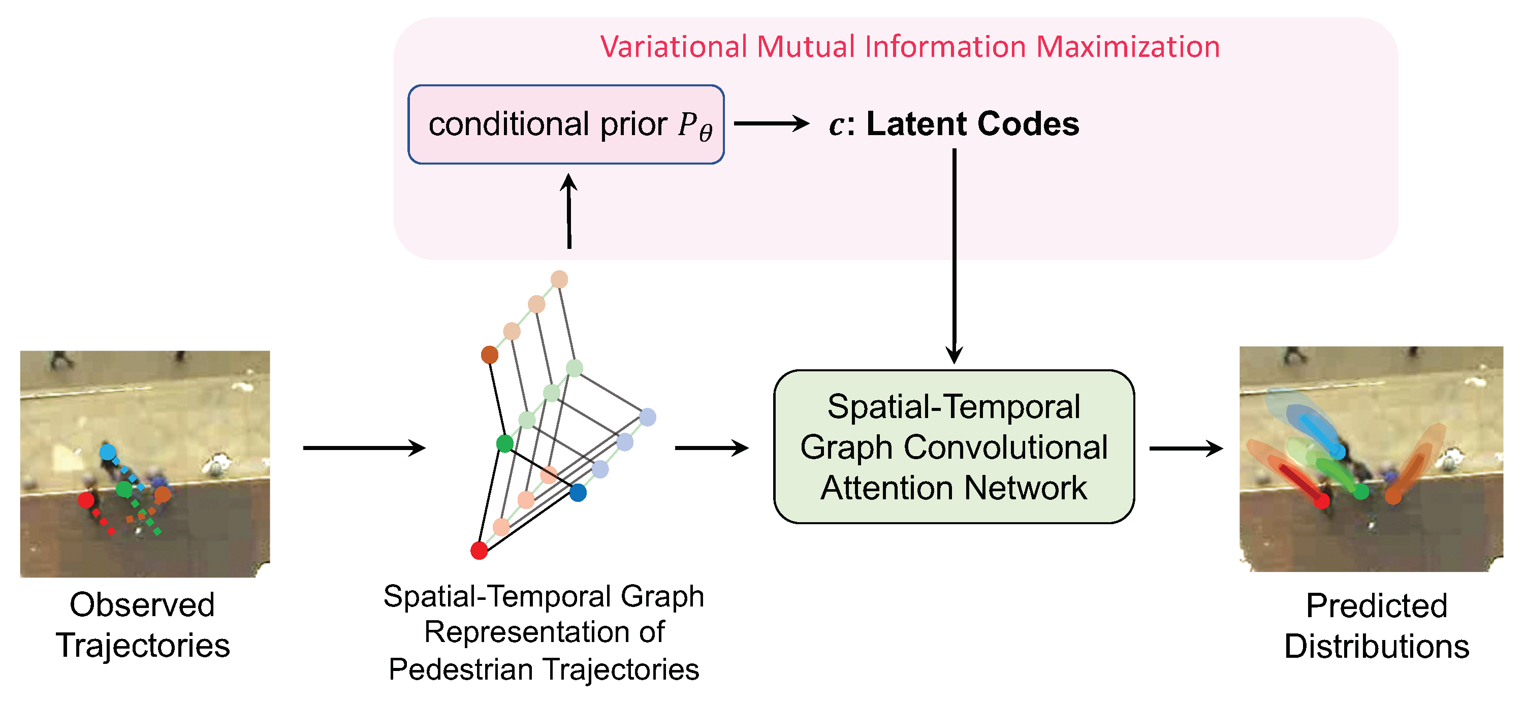
As depicted in Figure 2, there are two primary components at the core of our proposed method: the spatial-temporal graph network (Section 3.1) and variational mutual information maximization (Section 3.2). To begin with, we construct the spatial-temporal graph representation from the pedestrian trajectories (Section 3.1.1). Following this, the spatial-temporal graph convolutional attention network (STGCAN) comes into play. STGCAN serves a significant role in comprehensively modeling pedestrian interactions across both spatial and temporal dimensions. Delving deeper into its composition, this network is composed of two parts: spatial-temporal graph convolution (Section 3.1.2) and spatial-temporal graph attention (Section 3.1.3).

Figure 2.
The overview structure of the proposed method.
Spatial-temporal graph convolution applies convolution filters or kernels to the graph. On the other hand, spatial-temporal graph attention implicitly computes the relative weights among different nodes in a data-dependent way. For clearer differences and understanding how these two components work together to model pedestrian interactions, readers are directed to the end of Section 3.1.3.
For the second primary component, based on information theory, the technique of variational mutual information maximization (Section 3.2) helps to optimize the latent distribution through the proposed information-theoretic loss. Specifically, the model learns to predict an individual-level latent code for each pedestrian that possesses high mutual information with the future predicted trajectory. As a result, it enables the model to effectively capture the complexity and inherent heterogeneity of the pedestrian trajectories.
To summarize, the proposed approach is not only able to present a holistic view of their interactions but also able to capture the heterogeneity in pedestrian movements. Details regarding the optimization of the proposed method, including the multi-objective loss function, can be found in Section 3.3.
3.1. Spatial-Temporal Graph Convolutional Attention Network
3.1.1. Spatial-Temporal Graph Representation of Pedestrian Trajectories
To begin with, we need to construct the spatial-temporal graph representation from pedestrian trajectories. Essentially, a spatial-temporal graph is an attributed graph where the node attributes evolve through time [59]. The key idea behind the spatial-temporal graph is its capacity to simultaneously account for both spatial and temporal dependencies.
To build a spatial-temporal graph, we commence by formulating a sequence of spatial graphs. For every step t, a spatial graph is constructed to represent the locations of pedestrians within a given scene. Each is composed of three parts: a set of vertices , a set of edges , and an adjacency matrix , i.e., .
Elaborating further, the vertex set is given by , where each vertex represents a pedestrian. The edge set is composed of edges between two vertices, i.e., . Specifically, the edge represents whether the vertex and the vertex are connected or not. If and are connected, ; if and are not connected, . The adjacency matrix is defined as follows:
Each item () models the influence between the vertex and the vertex . As such, a spatial-temporal graph is finally constructed, consisting of a series of spatial graphs .
3.1.2. Spatial-Temporal Graph Convolution
Based on the spatial-temporal graph representation developed in Section 3.1.1, we introduce the spatial-temporal graph convolution (ST-GC) operation in this subsection. Before diving into the complete technical details of ST-GC, we start with a more general version of the convolution operation, which is on a two-dimensional grid or feature map.
In deep learning, neural networks that employ convolution operations are referred to as “convolutional neural networks (CNNs)” [49,53]. Typically, a CNN consists of multiple convolutional layers, and within each layer, multiple learnable filters or kernels are applied to the input feature map. These filters help to capture local patterns or features, enabling CNNs to learn hierarchical representations from the input data. Additionally, CNNs significantly benefit from the idea of “parameter sharing”, which reduces the number of parameters compared to fully connected layers.
For example, suppose the kernel size is equal to k, denotes the feature map at layer l, and denotes the feature map at layer . Through the training process, convolution operations are able to learn to aggregate the information from the neighbors centering around each location in . Therefore, the convolution operation on layer l can be summarized as:
where denotes the sampling function, represents the weight function at layer l, and denotes an activation function, e.g., ReLU or Sigmoid [53]. Note that the weight function is shared across different locations in .
Transitioning to the context of graph neural networks (GNNs), as different instances might have inconsistent structures, the convolution operation on graphs should be node-order agnostic [60,63,75,76,77]. As a result, some important modifications for convolution operations shown in Equation (5) are required. In consequence, the spatial-temporal graph convolution operation is formulated as follows:
where denotes the normalizing term, and
which denotes the neighbor set of the vertex . Specifically, denotes the minimum path connecting and , determines the spatial range of nodes to be contained in the neighbor set, and determines the temporal range of nodes to be contained in the neighbor set.
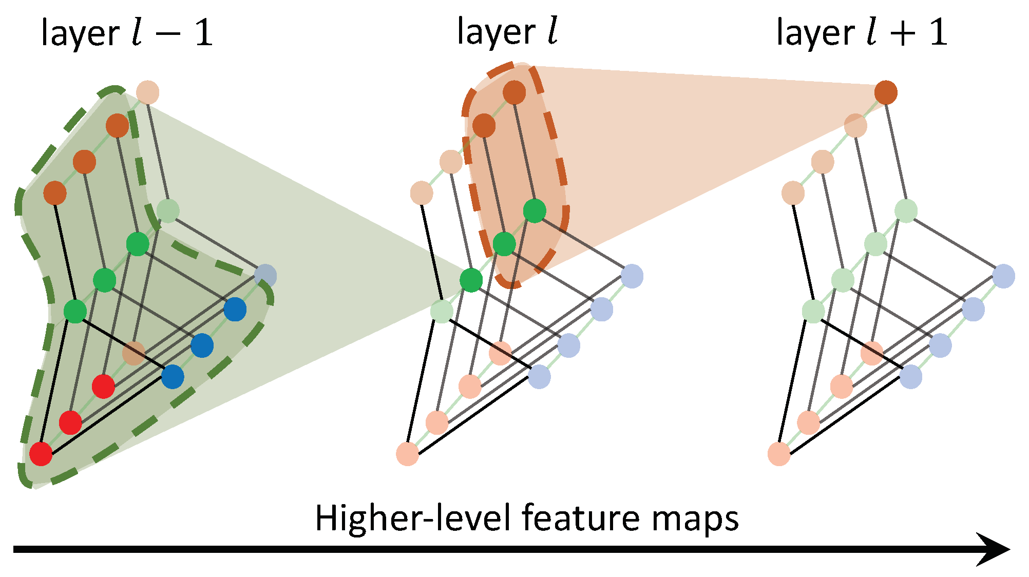
Based on the discussions above, the convolution operation on graphs can be defined by adapting the aforementioned formulation to scenarios where the input features map resides on a spatial-temporal graph. Figure 3 illustrates this concept, where nodes of different colors represent different pedestrians. In order to model how a certain pedestrian is walking in the future, information is aggregated from his or her past trajectories and the nearby pedestrians. As the feature map’s level increases, predictions utilize a greater number of pedestrians and longer temporal information.

Figure 3.
Multiple layers of spatial-temporal graph convolution (ST-GCN) will be applied and gradually generate higher-level feature maps on the graph.
3.1.3. Spatial-Temporal Graph Attention
We begin by introducing a generalized version of the attention mechanism and providing insights into its underlying principles. Following that, we elucidate our approach to investigating attention within the context of a spatial-temporal graph.
Generally, in urban environments, pedestrians tend to know which other pedestrians require their attention to prevent possible collisions. This intuitive awareness allows us humans to determine which pedestrians might pose a higher risk of collision and adjust our own paths accordingly to maintain a smooth and safe walking experience. Therefore, different pedestrians have different relative importance. Inspired by recent significant success [55,71,72,73,78], we leverage this principle by applying the “attention” mechanism to the constructed spatial-temporal graph.
Typically, an attention mechanism consists of three major components: a query, a key, and a value [72]. Intuitively speaking, the query is a representation of the current item or context that the model is trying to process. It serves as a reference for determining essential elements within the input data. The key represents an item in the input sequence, which the model compares with the query to determine their similarity or relevance. The value represents the significant information associated with each element in the input data.
The attention mechanism computes a score for each key–query pair, typically using a dot product, scaled exponential, or some other similarity function [71,72,73,79,80]. These scores are then passed through a softmax function and are converted into a probability distribution, which represents “the attention weights”. Intuitively speaking, when a weight between a query and a key is higher, the corresponding key–value pair is more important; thus, the attention mechanism pays more “attention” to this pair.
Finally, the attention mechanism computes a weighted sum of the values using the obtained attention weights, effectively selecting and aggregating the relevant information from different elements. This aggregated context vector is then used in subsequent layers of the model to make predictions. The process can be summarized into the following equation:
where is the dimension of each query, and the term can enhance the numerical stability of attention mechanisms.
In the context of GNNs, the previously mentioned three components, namely, a query, a key, and a value, are employed to learn meaningful representations of nodes, based on their local features and the structure of the underlying graph. As discussed in Section 3.1.1, each vertex represents a pedestrian, and represents pedestrian n at step t. We represent his or her corresponding query vector as , the key vector as , and the value vector as .
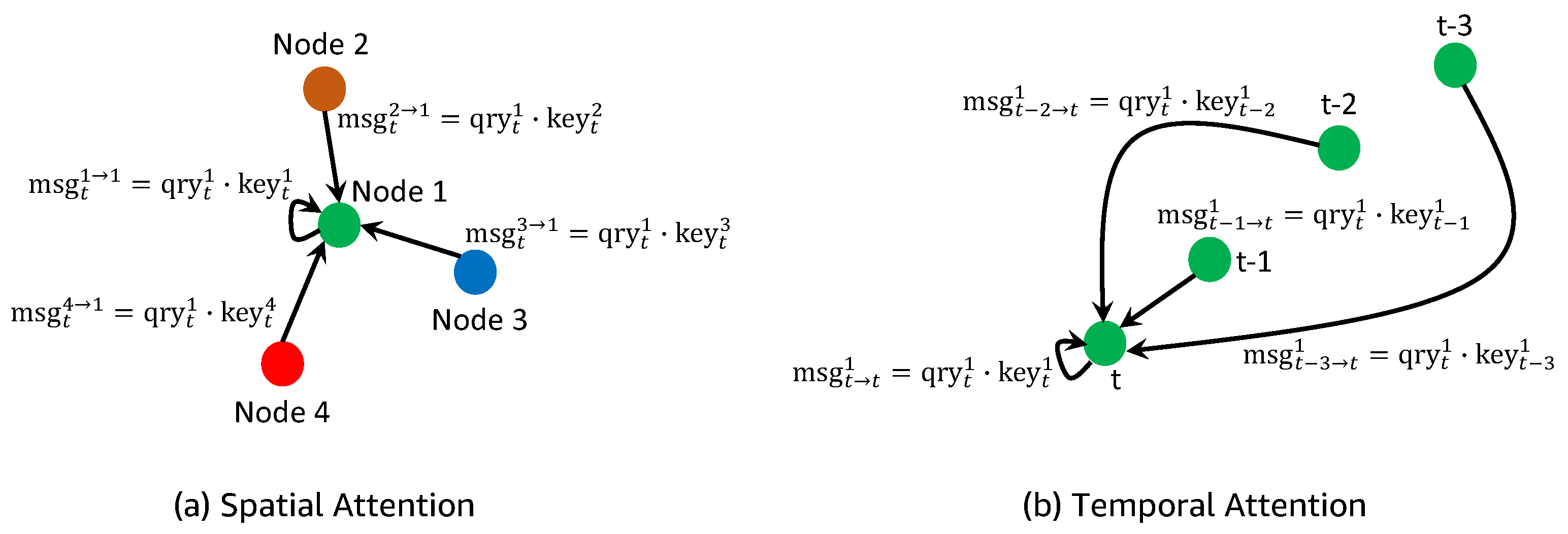
As illustrated in Figure 4, there are two major kinds of attention mechanisms in our framework: spatial attention and temporal attention. Both of them can be viewed as a way of message passing on a connected graph [73,81].

Figure 4.
stands for the message passed from node to , and stands for the temporal message of passed from to t. There are two primary types of attention mechanisms in our framework: spatial attention and temporal attention. (a) Spatial attention models the crowd as a graph and helps to predict a pedestrian’s trajectory based on the movements of her or his neighboring pedestrians. (b) Temporal attention, on the other hand, focuses on each individual pedestrian and primarily assists in capturing her or his trajectory trends over time.
Spatial attention focuses more on message exchanges among nodes within the same time step. Intuitively speaking, it helps to generate feasible trajectories by aggregating information from other pedestrians. Suppose the message passed from node to is , which is defined as:
and based on Equation (8), we may formulate spatial attention as:
On the other hand, temporal attention focuses more on the process of temporal message passing by aggregating information through the relevant time steps. Intuitively speaking, it helps to generate feasible trajectories by incorporating the temporal significant features of pedestrians.
Here, we show how the temporal message of passed from to t:
and based on Equation (8), we may formulate temporal attention as follows:
Difference Between ST-GC and ST-GAT Spatial-temporal graph convolution (ST-GC) and spatial-temporal graph attention (ST-GAT) are two commonly used techniques in GNNs. Both of them can learn meaningful representations of pedestrian trajectories through the spatial and temporal dimensions. Their major difference lies in how they aggregate information from neighboring nodes.
- In ST-GC, information from neighboring nodes is communicated by applying convolution filters or kernels on the graph, which typically involves a weighted sum of features across neighboring nodes. Usually, those weights can be identical (e.g., GraphSAGE [63]), predetermined, or learnable ([60,70]). Therefore, the weights are considered to be “explicitly” assigned to the neighborhoods of the focused node during the aggregation process [59].
- However, in ST-GAT, the weights between two connected nodes are considered to be “implicitly” computed. Specifically, those weights are learned based on the similarity of their feature representations, which takes into account the relative importance for different node pairs [59,73]. Typically, more important nodes tend to have higher similarity scores, resulting in them being assigned larger weights.
Social Interaction Modeling In this subsection, based on the discussed ST-GC and ST-GAT, we aim to clarify how they capture the modeling of pedestrian social interactions.
As introduced in Section 3.1.1, the adjacency matrix can be considered as a representation of the graph edge attributes. In the spatial-temporal graph convolution part, we incorporate our prior knowledge about the social relations among different pedestrians into a kernel function, e.g., pedestrians closer in distance tend to be more important. The kernel function maps node attributes at and to the attribute value , which is defined as follows:
Equation (13) is consistent with the intuition that pedestrians are more likely to be influenced by each other if they are closer. Additionally, the kernel function is symmetric:
However, since the form of the kernel function is predetermined, and some pedestrian interactions are asymmetric, the interaction modeling in a purely spatial-temporal graph convolution-based model might be insufficient. Therefore, we integrate the spatial-temporal graph attention mechanism into our model. As discussed in Section 3.1.3, the relative importance of pedestrian m to pedestrian n is data-dependent, which is determined by the value of . Therefore, there is not any predetermined kernel in the the spatial-temporal graph attention mechanism. Generally, the spatial-temporal graph attention mechanism is able to capture the asymmetric importance:
which stems from the fact that, in general, and .
3.2. Variational Mutual Information Maximization
In real-world scenarios, when a pedestrian encounters other pedestrians, their reactions can vary from person to person. This variance can be influenced by factors like age, with different age groups having distinct walking behaviors [24]. Furthermore, an individual’s walking preference might have notable changes depending on whether walking alone or in a group [22,25]. Although few frameworks have been employed to produce such diverse trajectory styles (e.g., the variety loss [34]), there is still a need to understand how to effectively capture the intrinsic heterogeneity within the pedestrian trajectories.
In this subsection, to solve the mentioned issue, we introduce the technique of variational mutual information maximization. We begin by considering the principles of information theory [82,83,84,85]. Suppose X and Y are random variables. If we want to measure the “amount of information” learned about Y by providing the knowledge of X or vice versa, mutual information is utilized. The mutual information can be expressed as the difference between the self-entropy of Y and the conditional entropy of Y given X:
where denotes the self-entropy of X, and denotes the self-entropy of Y. denotes the conditional entropy of X given Y, and denotes the conditional entropy of Y given X.
The conditional mutual information is defined as below:
Intuitively speaking, can be treated as how much uncertainty is reduced in X when Y is observed, given Z. If X and Y are independent, the knowledge of X does not provide any information about Y and vice versa. As a result, the mutual information between X and Y is zero. However, given Z, if the knowledge of X provides extensive information about Y, then can be extremely high.
This interpretation helps to formulate the idea: given the past trajectory , in order to learn meaningful representations for the future pedestrian trajectory, there should be high conditional mutual information between the latent code and the generated trajectory . In other words, should be high. As such, we propose an information-theoretic loss:
However, in practice, directly maximizing the mutual information is extremely challenging, as it requires the truth unknown posterior . Therefore, we utilize a common technique in statistics and machine learning to address this problem, i.e., variational inference [85,86,87,88]. By defining an approximate posterior over the original unknown posterior , we are able to construct a lower bound over the original quantity :
where G is the abbreviation for , stands for the Kullback–Leibler (KL) divergence, and the last step holds true because KL divergence is always always non-negative [82,84]. Therefore, we may construct a lower bound over the original objective Equation (21):
As the approximate posterior approaches the true posterior distribution , approaches zero. Therefore, the lower bound approaches the mutual information and becomes tighter. It is worth mentioning that we also optimize the conditional entropy of the latent code , so that we the latent variable distribution and the predictor are learned simultaneously.
To summarize, the final objective of the variational mutual information maximization part can be written as:
where is the conditional prior distribution for the latent code .
The primary differences between Equation (20) and the mutual information-inspired objective in [85] are:
- In ref. [85], there is only one latent code for each training example. However, in this paper, there are multiple latent codes for each training example. Different pedestrians may have distinct preferences and walking styles. It is generally infeasible to assume all pedestrians follow the same preference or walking style. Therefore, for each pedestrian n, he or she has its own latent code , and different pedestrians generally have different latent codes, allowing the proposed framework to effectively model the latent patterns in pedestrian trajectories.
- In this paper, the proposed information-theoretic loss is based on the conditional mutual information. However, in ref. [85], the loss is based on the mutual information.
- Different from the previous research taken in [85], where the prior latent code distribution is assumed to be fixed, we opt to optimize the prior distribution as well.
3.3. Multi-Objective Loss Function
To optimize the proposed method, we utilize the multi-objective loss defined below:
where denotes the prediction loss, denotes the generative adversarial loss, and denotes the information loss. , and control the relative importance of each loss.
- : The prediction loss relies on negative log-likelihood, which is defined as:where . Intuitively speaking, when is decreasing, the log-likelihood of is increasing. The model and the posterior distribution together are encouraged to accurately predict the ground-truth future trajectory.
- : The generative adversarial loss relies on the generator G and the discriminator D, in which two models are jointly trained. The generator G captures the distribution for the future trajectory, and the discriminator distinguishes whether a sample comes from the training data or the generator G.
- : The information-theoretic loss relies on the conditional prior distribution , the model , and the approximate posterior , which has been discussed in Section 3.2.
Notably, in order to enable effective backpropagation through the discrete latent code, we utilize the Gumbel–Softmax reparameterization trick [89,90]. Basically, the sampling process from a categorical distribution is usually non-differentiable. The Gumbel-Softmax reparameterization allows us to relax the discrete sampling process into a continuous and differentiable one, thereby enabling gradient-based optimization.
To summarize, the pipeline depicted in Figure 5 outlines the primary structure of our proposed framework, and Algorithm 1 describes the training procedure. Initially, a spatial-temporal graph is constructed from the pedestrian trajectories. Following this, spatial-temporal graph convolution (ST-GC) and spatial-temporal graph attention (ST-GAT) are deployed to extract meaningful information from pedestrian interactions in both spatial and temporal dimensions. In the meantime, latent codes will be inferred for all pedestrians, enabling the model to capture the intrinsic heterogeneity within their trajectories, and forecast their future paths. The optimization process integrates the prediction loss, the generative adversarial loss, and the information loss, which helps to achieve a more accurate and reliable result.
| Algorithm 1: Training Procedure of InfoSTGCAN |
|

Figure 5.
The structure of our proposed method. We model pedestrian interactions through the integration of spatial-temporal graph convolution and spatial-temporal graph attention. By leveraging the conditional prior distribution and the approximate posterior , individual-level latent codes are estimated so that inherent heterogeneity in pedestrians’ behavior preferences can be properly captured.
4. Experiments and Results
In this section, we first outline the experimental settings, including the datasets and evaluation metrics. Subsequently, we delve into the implementation details, present the experiment results, provide a comprehensive analysis of these results, and conclude with ablation studies.
4.1. Datasets and Evaluation Metrics
Datasets The proposed method is evaluated on multiple publicly accessible datasets: ETH [91] and UCY [92]. The ETH dataset contains approximately 750 different pedestrians and is divided into two scenarios: ETH and HOTEL. The UCY dataset contains approximately 786 unique pedestrians and is divided into three scenarios: ZARA1, ZARA2, and UNIV. These datasets consist of real-world pedestrian trajectories with complex human interactions. Specifically, lots of challenging pedestrian behaviors are covered in the datasets, such as pedestrians crossing each other, walking together, avoiding collision, and groups assembling and disbanding [91]. In accordance with a similar strategy utilized in previous studies [27,34], all trajectories are sampled every 0.4 s.
Evaluation Metrics In accordance with prior work [27,34,57,93], we choose to use the following evaluation metrics:
- Average Displacement Error (ADE): The average distance between the predicted trajectory and the ground truth trajectory across all time steps, which is defined as follows:where are the real locations, and are the predicted locations.
- Final Displacement Error (FDE): The distance between the predicted final destination and the true final destination at the end of the prediction period , which is defined as follows:
Intuitively speaking, different metrics serve as different purposes. ADE evaluates the average prediction error across the whole trajectory, whereas FDE focuses solely on the prediction error at the destination.
4.2. Implementation Details
In this section, we provide important details on appropriately implementing the proposed model. To facilitate the learning process [60,70], we normalize the adjacency matrix at each time step t as follows:
where I is an identity matrix, which serves to add self-connections to all nodes. is the diagonal node degree matrix of . We use to denote the stack of all adjacency matrices , and to denote the stack of matrices . Suppose the vertices values at the layer l as , which is a stack of vertices values across all steps . We can now employ the matrices defined to implement the ST-GC layers:
where represents the learnable parameters at the l-th layer. The above Equation (38) follows similar ideas in [57,70].
Model Architecture and Training Setup The proposed model consists of a series of ST-GC and ST-GAT layers, which helps to extract spatial-temporal node embeddings from the input data. Later, those node embeddings are concatenated with latent codes, and then, several convolutional layers are followed such that the output time dimension is manipulated to match the length of predicted horizon .
Unless noted otherwise, we choose to use PReLU [94] as the activation function through our model. During training, we used a batch size of 128 and the default optimizers were chosen to use Stochastic Gradient Descent (SGD). The initial learning rate was 0.01, and it was decreased based on exponential scheduling with a decay factor 0.97. To prevent overfitting to the training data, we randomly dropped out the features at a probability of 0.5.
4.3. Results Analysis
In this subsection, we begin by comparing our results with baseline models. Subsequently, we provide a comprehensive qualitative analysis of how our proposed method models pedestrian interactions and takes heterogeneous behavior choices into account. We illustrate cases where InfoSTGCAN successfully predicts collision-free trajectories for scenarios such as pedestrians walking in the same direction, approaching from opposing directions, or merging at angles. Moreover, our model is able to generate socially acceptable trajectories based on the predicted personalized latent codes.
4.3.1. Comparison with Baseline Models
Baselines We compare the proposed method with the following baselines:
- Linear: A linear regression model characterized by minimizing the least square error.
- Social LSTM (S-LSTM) [27]: An LSTM approach that incorporates the “social pooling” mechanism for hidden states.
- S-GAN-Pooling [34]: A GAN-based approach that utilizes global pooling for pedestrian interactions.
- SR-LSTM-2 [29]: An LSTM-based method that leverages a state refinement technique.
- GAT [55]: A graph attention network leveraging the sequence-to-sequence architecture.
- Sophie [35]: A GAN-based method that takes both scene and social factors into account through a dual attention mechanism.
- SCAN [58]: An LSTM-based encoder–decoder framework that incorporates a novel spatial attention mechanism to predict trajectories for all pedestrians.
- Social-STGCNN [57]: A spatial-temporal graph-based approach that employs a spatial-temporal graph convolutional network to handle complex social interactions.
The performance of the proposed method is evaluated against other benchmark models on ADE/FDE metrics, as presented in Table 2. In general, our method outperforms all baseline methods on the two metrics. Our proposed model achieves an error of 0.62 on the average FDE metric, representing an approximate 20% improvement over the previous best performance (0.75). For the average ADE metric, the proposed model is better than the previous best performance by 5%. Interestingly, although our model does not need the vision signal containing scene context information, it can still outperform methods that utilize such information, such as SR-LSTM and Sophie.

Table 2.
ADE/FDE metrics for several baselines and our method on all the datasets. All methods are evaluated with an observation length of 8 frames (3.2 s) and a prediction horizon of 12 frames (4.8 s). The model with lower values of metrics has a better performance.
4.3.2. Results Visualization
Figure 6 illustrates the validation losses over successive epochs for the considered datasets, where the x-axis corresponds to the training epoch index, and the y-axis represents the value of the validation loss. Each line in the figure represents the progression of the validation loss for a specific dataset. As observed from Figure 6, the proposed method exhibits convergence across all datasets.
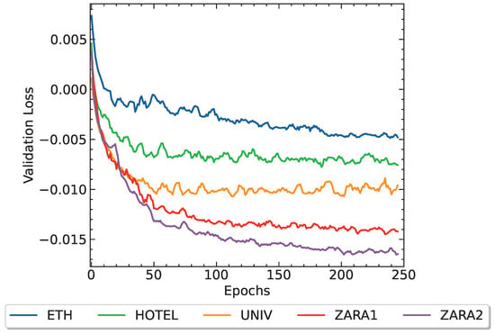
Figure 6.
The validation loss calculated for each dataset vs. number of epochs.
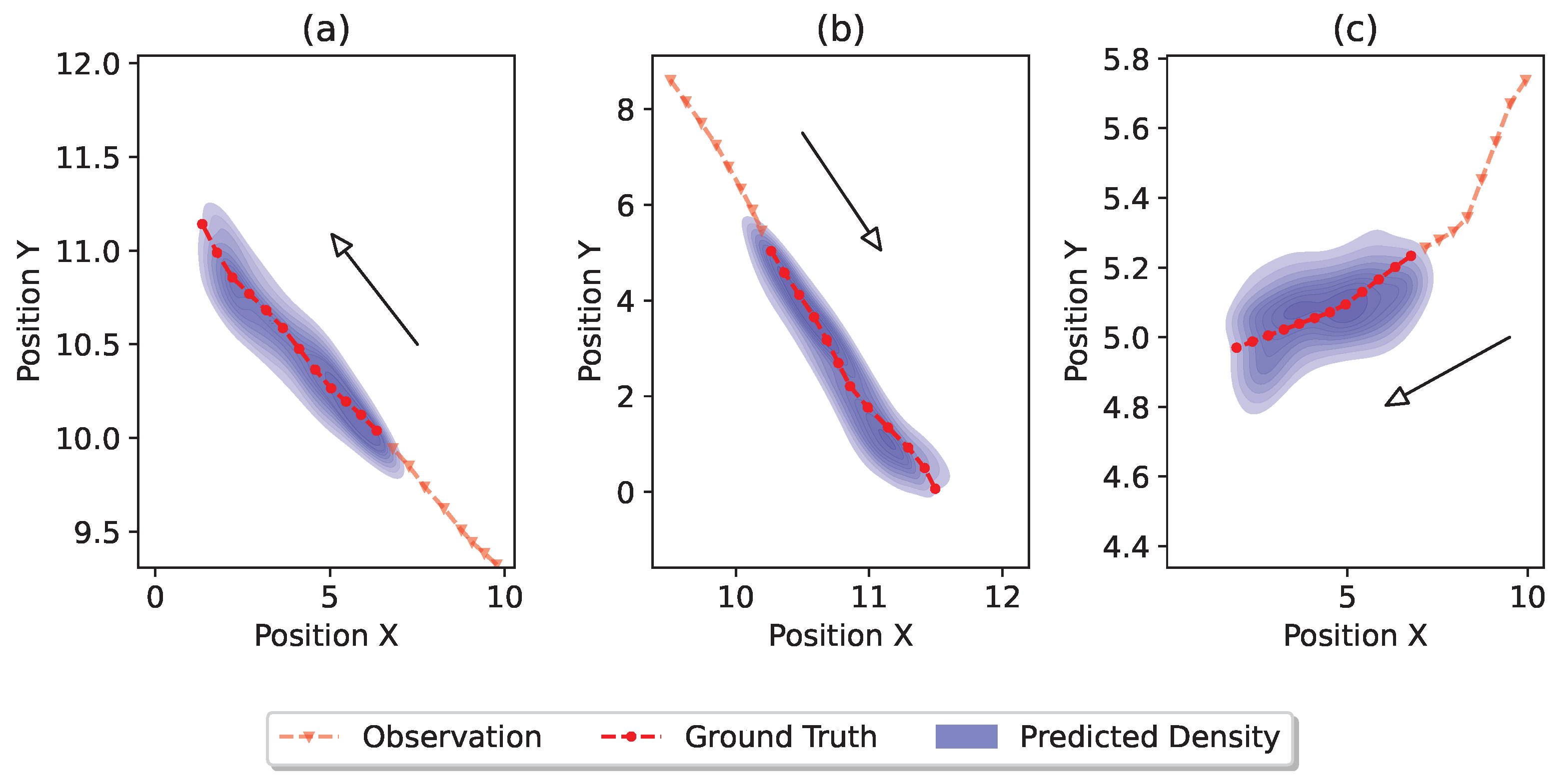
In Figure 7, we present multiple qualitative examples and the trajectory distributions generated by our proposed method. In Figure 7a,b, pedestrians are moving straight in different directions. Our model successfully captures these trends, and accurately covers the ground truth future trajectory. In Figure 7c, the pedestrian makes an initial right turn before proceeding straight. As the observed trajectory in (c) is more curved compared to the trajectories in (a,b), we observe a broader predicted distribution. This broader prediction is intuitive, since a turn in the observed trajectory increases uncertainty, making the accurate prediction of the future trajectory more challenging.
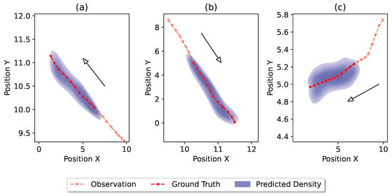
Figure 7.
Visualization of the distributions of the predicted trajectories. Different sub-figures (a–c) represent different scenarios. For each scenario, the dashed red line with triangle markers denotes the observed trajectory, the dashed red line with circle markers denotes the ground truth trajectory, and the blue density represents the predicted trajectory distribution.
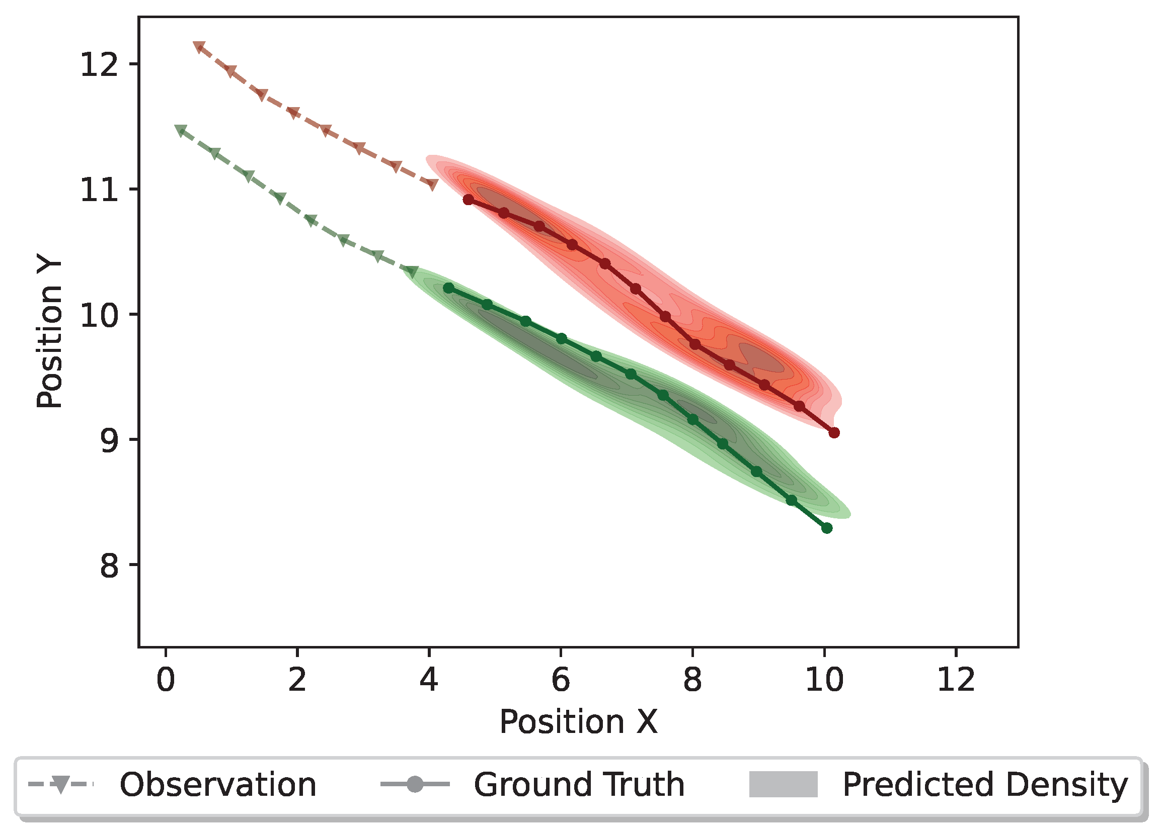
Additionally, we present the trajectory distributions for the scenarios of multi-pedestrian interactions in Figure 8 and Figure 9. Figure 8 depicts a scenario where two pedestrians are walking together in parallel from the same direction. Typically, when pedestrians are walking together in parallel, their connections are usually tight and their momentum should be preserved in the future. Predictions generated by InfoSTGCAN support this observation, indicating that both pedestrians are likely to continue walking in parallel without colliding. Additionally, the predicted density demonstrates a close alignment with the ground truth trajectory.
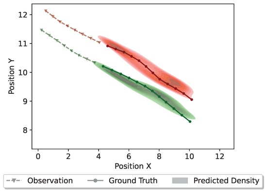
Figure 8.
Distributions of the predicted trajectories for two pedestrians walking together from the same direction. Different colors denote different pedestrians. The dashed line with triangle markers denotes the observed trajectory, the solid line with circle markers denotes the ground truth trajectory, and the colorful density represents the predicted trajectory distribution.
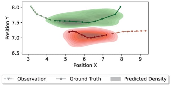
Figure 9.
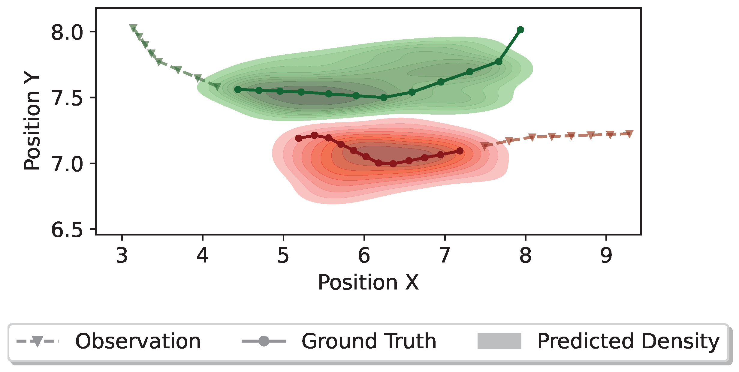
Distributions of the predicted trajectories for two pedestrians meeting from different directions. Different colors denote different pedestrians. The dashed line with triangle markers denotes the observed trajectory, the solid line with circle markers denotes the ground truth trajectory, and the colorful density represents the predicted trajectory distribution.
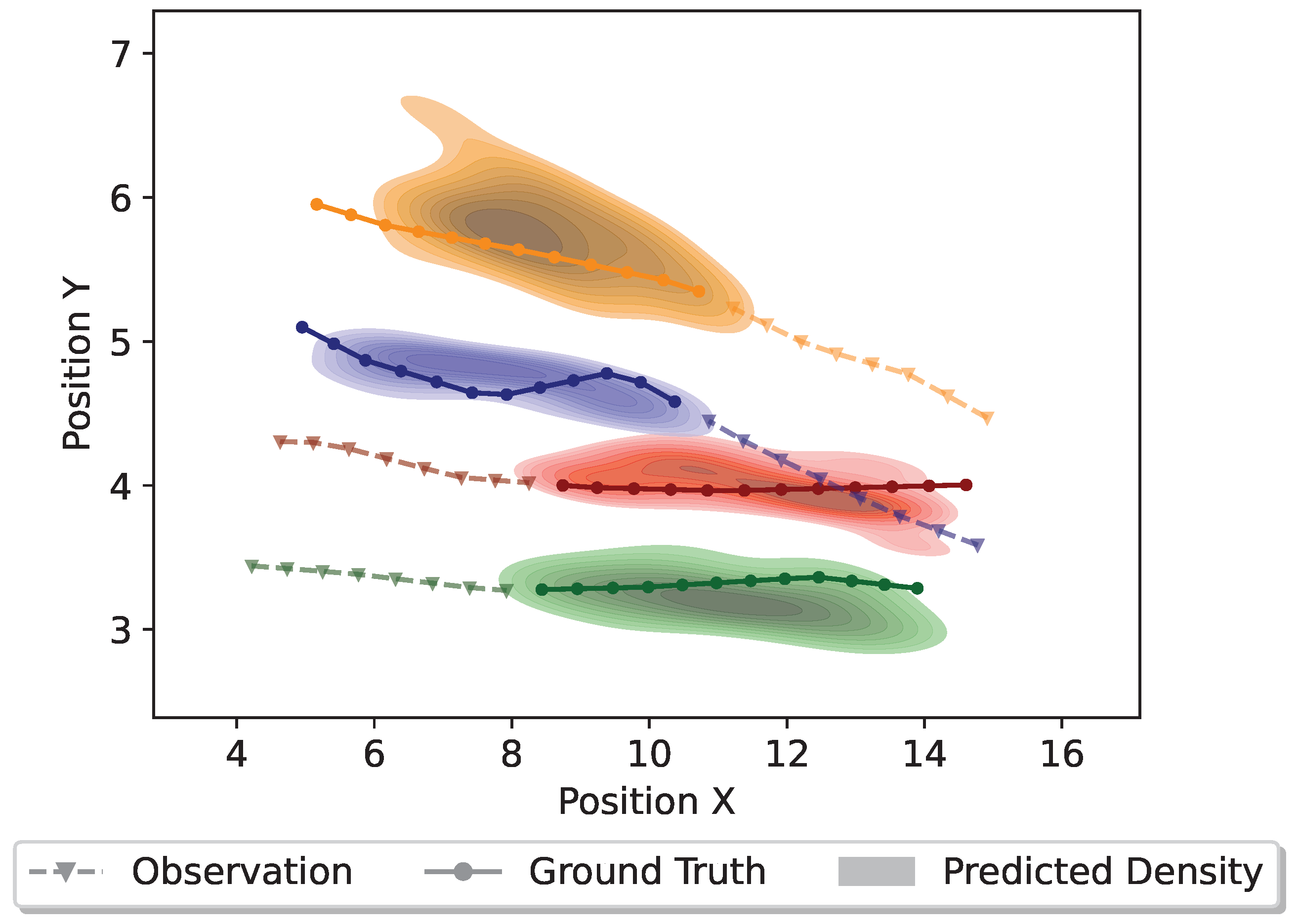
On the other hand, Figure 9 depicts a scenario where two pedestrians are approaching each other from different directions. If both pedestrians maintain their original directions and momentum, a collision could happen. Accordingly, such a scenario requires the proposed model to generate plausible collision-free trajectories. The finding suggests that the proposed model achieves it effectively by capturing the social dynamics among different pedestrians. Furthermore, Figure 10 illustrates a scenario involving four pedestrians meeting from different directions.
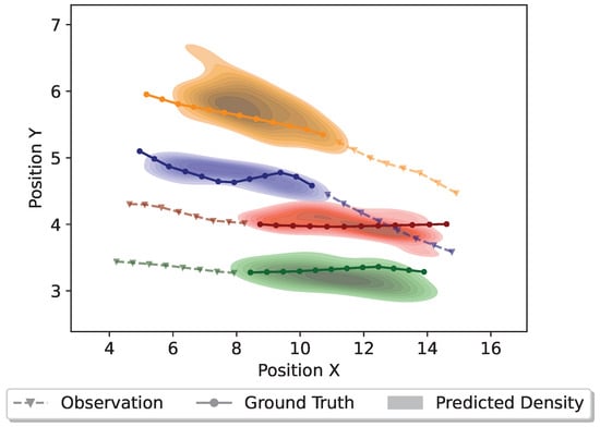
Figure 10.
Distributions of the predicted trajectories for four pedestrians meeting from different directions. Different colors denote different pedestrians. The dashed line with triangle markers denotes the observed trajectory, the solid line with circle markers denotes the ground truth trajectory, and the colorful density represents the predicted trajectory distribution.
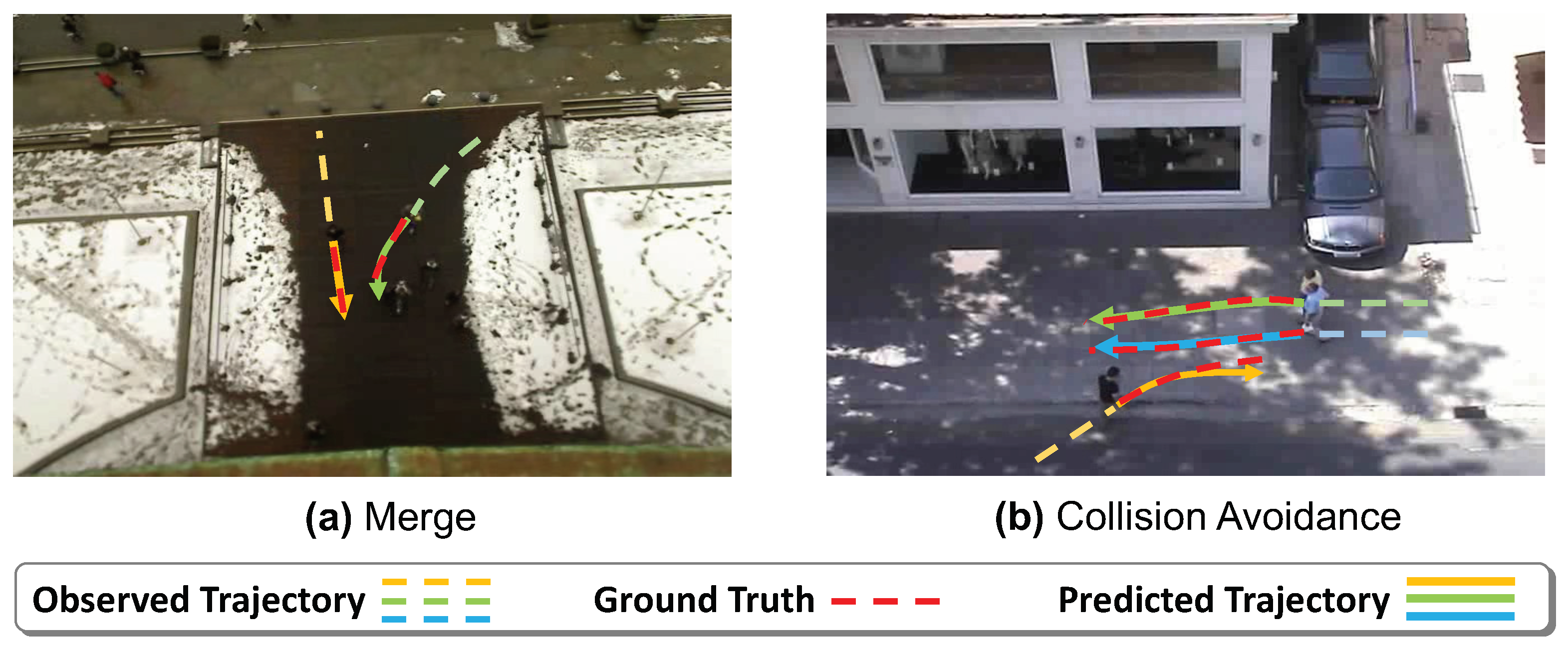
In order to gain a comprehensive understanding of the quality of samples generated by the proposed method, we visualize the trajectories sampled from the predicted bi-variate Gaussian distributions. As shown in Figure 11, there are two scenarios. In the first scenario (Figure 11a), two pedestrians merge at an angle, and the result demonstrates our model’s capability to properly predict the trajectories for this situation. In the second scenario (Figure 11b), the pedestrian in orange attempts to avoid potential collisions with other two pedestrians who are walking together. The results indicate that the model is able to correctly predict the trajectories for all three pedestrians involved in this scenario. This analysis shows that the samples generated by the proposed method can encapsulate different social behaviors of pedestrians.
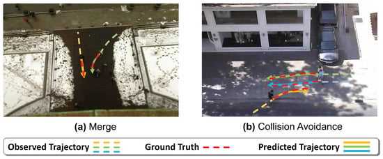
Figure 11.
Examples of predictions from our model. Scenario (a) shows that our model can properly predict the trajectories for two pedestrians merging at an angle. Scenario (b) shows that our model learns to predict a socially acceptable trajectory for the pedestrian in orange without collisions.
4.3.3. Interpretable Latent Representation
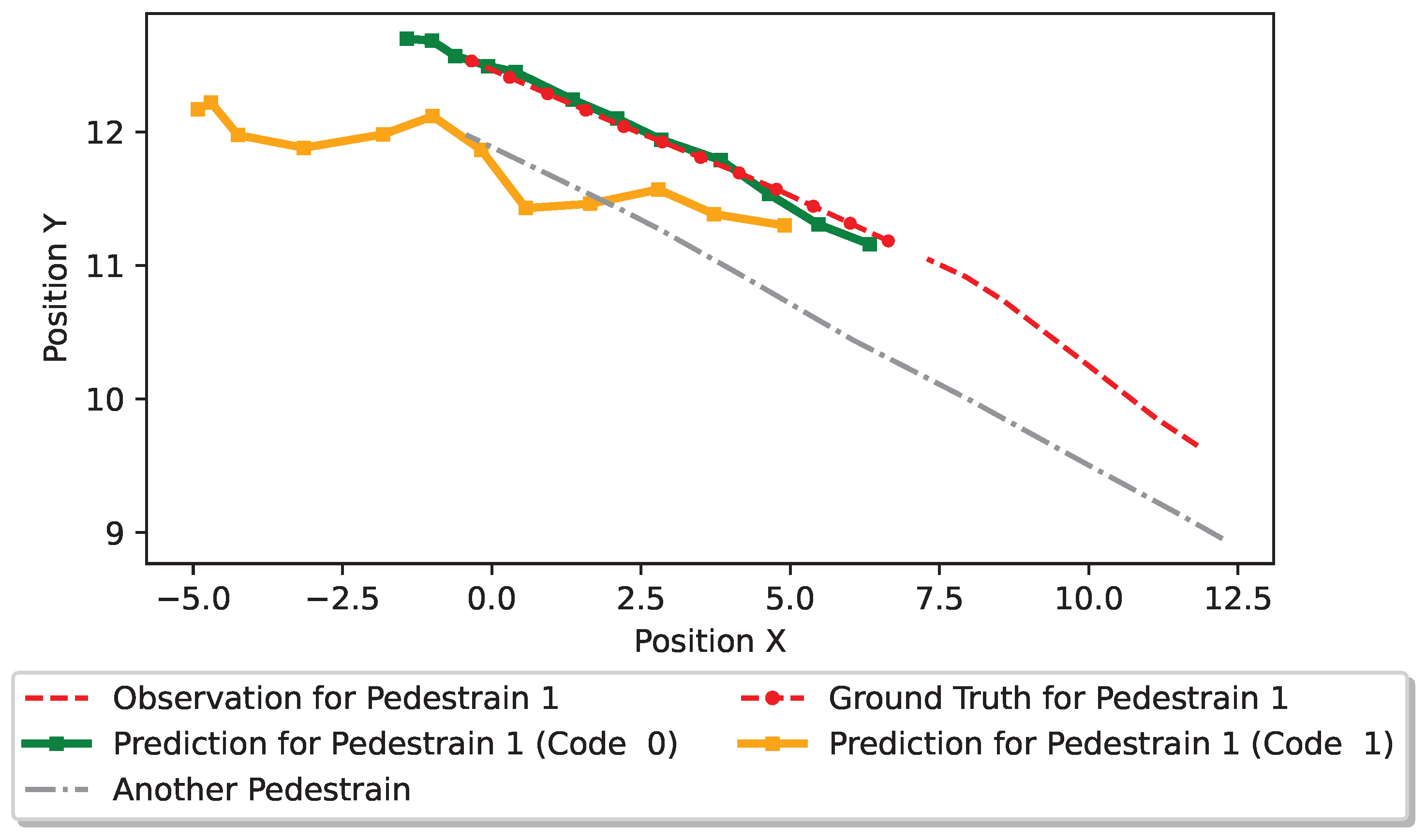
As illustrated in Figure 12, we compare the generated trajectories from different latent codes. When the spatial-temporal network needs to generate trajectories, pedestrians’ latent codes have to be provided. Therefore, different latent codes may generate different trajectories. Both code 0 and code 1 are sampled from the learned conditional prior distribution , with code 0 exhibiting a higher likelihood than code 1. As depicted in Figure 12, the trajectory generated when applying code 0 typically follows a straight path, whereas that induced by code 1 tends to turn left.

Figure 12.
Visualizations of generated trajectories from different latent codes. Code 0 has a higher likelihood than code 1.
In the context of pedestrian interaction, the trajectory generated by code 1 may result in collisions with the other pedestrian (in gray). The trajectory generated by code 0 is better aligned with the ground truth trajectory without potential collisions. As such, code 0 is more desirable and has a higher predictive likelihood than code 1. This evidence indicates that our framework is able to generate satisfied trajectories through learning a personalized latent code for each individual pedestrian.
4.4. Ablation Study
We conduct a series of comparative experiments to validate the efficacy of our proposed method by examining different values of in the multi-objective loss function . As discussed in Section 3.3, the multi-objective loss function is defined as . Through these experiments, two primary goals are addressed:
- Demonstrate the crucial role of the GAN loss part.
- Highlight the significance of maintaining a balanced weight between and .
According to the results presented in Table 3, omitting the GAN loss by setting leads to a decline in performance. More specifically, when we exclude the GAN loss, it effectively means removing the discriminator from the architecture. This underscores the importance of the GAN loss component within the multi-objective loss function.

Table 3.
The ablation study on . Multiple different values are tested to show the model performance on the HOTEL dataset.
Additionally, as shown in Table 3, when we overemphasize or downplay by setting the weight ratio , the model potentially underestimates the importance of accurately predicting the ground-truth future trajectory. Therefore, a balanced weight on resulted in an appropriate focus on the final prediction accuracy, which is desirable.
These findings validate the importance of the GAN loss component and the significance of maintaining a balanced weight between the prediction loss and the information loss for optimal performance.
5. Conclusions and Future Research
In this paper, we formulate the task of pedestrian trajectory prediction as a spatial-temporal graph and develop a novel pedestrian trajectory prediction model, InfoSTGCAN. The proposed model takes into account both pedestrian interactions and heterogeneous behavior choices. Specifically, to better model pedestrian interactions, our proposed model consists of two parts, spatial-temporal graph convolution and spatial-temporal graph attention, enabling the analysis of interactions through a combination of prior knowledge and data-driven methods. To address the heterogeneity within the pedestrian behavior choices, we utilize the variational mutual information maximization technique, which is primarily composed of a conditional prior distribution and an approximate posterior distribution.
The proposed method outperforms baseline models across several publicly accessible datasets. Visualization of the generated trajectories reveals our method’s capacity to handle various scenarios, including pedestrians going straight from different directions or making a right turn first and then going straight. We also conduct a qualitative analysis of the proposed method in different situations, such as collision avoidance, parallel walking, and pedestrians merging. In these situations, InfoSTGCAN tends to generate realistic collision-free trajectories. Additionally, we show that our framework is able to generate satisfactory trajectories through learning a personalized pedestrian-level latent code.
Nevertheless, we identify several promising future directions that are worth exploring further. The first aspect involves exploring more metrics related to probabilistic trajectory prediction beyond the standard ADE/FDE for training and evaluation, e.g., Mahalanobis distance [95]. Secondly, our methodology currently models pedestrian social interactions through ST-GC and ST-GAT; an exciting direction is to integrate more socially aware or physics-based methods [96]. Lastly, the third aspect refers to an integrative approach that combines heuristic optimization [97], causal inference [22,23,26] or clustering techniques [98].
Author Contributions
Conceptualization, K.R.; methodology, K.R.; software, K.R.; validation, K.R.; formal analysis, K.R.; investigation, K.R.; resources, K.R.; writing—original draft preparation, K.R.; writing—review and editing, K.R. and X.D.; visualization, K.R.; supervision, X.D.; project administration, X.D.; funding acquisition, X.D. All authors have read and agreed to the published version of the manuscript.
Funding
This work is partially sponsored by the National Science Foundation (NSF) under the Smart and Connected Communities (S&CC) award CMMI-2218809.
Data Availability Statement
All data are contained within the article.
Conflicts of Interest
The authors declare no conflicts of interest.
Abbreviations
The following abbreviations are used in this manuscript:
| Major Notations | |
| Trajectory | |
| N | number of pedestrians |
| observed trajectory for the pedestrian | |
| future ground-truth trajectory for the pedestrian | |
| length of observed trajectories | |
| length of predicted trajectories | |
| random variables describing the location of the pedestrian at time step t | |
| predicted location of the pedestrian at time step t | |
| Spatial-Temporal Graph | |
| spatial graph at step t | |
| spatial-temporal graph | |
| set of vertices for | |
| set of edges for | |
| adjacency matrix for | |
| I | identity matrix |
| Variational Mutual Information Maximization | |
| G | generator |
| D | discriminator |
| conditional prior distribution for the latent code | |
| posterior distribution for the latent code | |
| approximate posterior distribution for | |
| Spatial-Temporal Graph Convolution | |
| feature map at layer l | |
| feature map at layer | |
| sampling function | |
| weight function at layer l | |
| Spatial-Temporal Graph Attention | |
| Qry | query of the attention mechanism |
| Key | key of the attention mechanism |
| Val | value of the attention mechanism |
References
- Hashimoto, Y.; Gu, Y.; Hsu, L.T.; Iryo-Asano, M.; Kamijo, S. A probabilistic model of pedestrian crossing behavior at signalized intersections for connected vehicles. Transp. Res. Part C Emerg. Technol. 2016, 71, 164–181. [Google Scholar] [CrossRef]
- Haghani, M. Empirical methods in pedestrian, crowd and evacuation dynamics: Part I. Experimental methods and emerging topics. Saf. Sci. 2020, 129, 104743. [Google Scholar] [CrossRef]
- Bahari, M.; Nejjar, I.; Alahi, A. Injecting knowledge in data-driven vehicle trajectory predictors. Transp. Res. Part C Emerg. Technol. 2021, 128, 103010. [Google Scholar] [CrossRef]
- Kalatian, A.; Farooq, B. A context-aware pedestrian trajectory prediction framework for automated vehicles. Transp. Res. Part C Emerg. Technol. 2022, 134, 103453. [Google Scholar] [CrossRef]
- Bautista-Montesano, R.; Galluzzi, R.; Ruan, K.; Fu, Y.; Di, X. Autonomous navigation at unsignalized intersections: A coupled reinforcement learning and model predictive control approach. Transp. Res. Part C Emerg. Technol. 2022, 139, 103662. [Google Scholar] [CrossRef]
- Mo, Z.; Li, W.; Fu, Y.; Ruan, K.; Di, X. CVLight: Decentralized learning for adaptive traffic signal control with connected vehicles. Transp. Res. Part C Emerg. Technol. 2022, 141, 103728. [Google Scholar] [CrossRef]
- Wang, Z.; Sun, P.; Hu, Y.; Boukerche, A. A novel mixed method of machine learning based models in vehicular traffic flow prediction. In Proceedings of the 25th International ACM Conference on Modeling Analysis and Simulation of Wireless and Mobile Systems, Montreal, QC, Canada, 24–28 October 2022; ACM: New York, NY, USA, 2022; pp. 95–101. [Google Scholar]
- Fu, Y.; Di, X. Federated Reinforcement Learning for Adaptive Traffic Signal Control: A Case Study in New York City. In Proceedings of the 2023 IEEE 26th International Conference on Intelligent Transportation Systems (ITSC), New York, NY, USA, 24–28 September 2023; IEEE: New York, NY, USA, 2023; pp. 5738–5743. [Google Scholar]
- Musleh, B.; García, F.; Otamendi, J.; Armingol, J.M.; De la Escalera, A. Identifying and tracking pedestrians based on sensor fusion and motion stability predictions. Sensors 2010, 10, 8028–8053. [Google Scholar] [CrossRef] [PubMed]
- Zangenehpour, S.; Miranda-Moreno, L.F.; Saunier, N. Automated classification based on video data at intersections with heavy pedestrian and bicycle traffic: Methodology and application. Transp. Res. Part C Emerg. Technol. 2015, 56, 161–176. [Google Scholar] [CrossRef]
- St-Aubin, P.; Saunier, N.; Miranda-Moreno, L. Large-scale automated proactive road safety analysis using video data. Transp. Res. Part C Emerg. Technol. 2015, 58, 363–379. [Google Scholar] [CrossRef]
- Errico, F.; Crainic, T.G.; Malucelli, F.; Nonato, M. A survey on planning semi-flexible transit systems: Methodological issues and a unifying framework. Transp. Res. Part C Emerg. Technol. 2013, 36, 324–338. [Google Scholar] [CrossRef]
- Grahn, R.; Qian, S.; Hendrickson, C. Improving the performance of first-and last-mile mobility services through transit coordination, real-time demand prediction, advanced reservations, and trip prioritization. Transp. Res. Part C Emerg. Technol. 2021, 133, 103430. [Google Scholar] [CrossRef]
- Ma, X.; Karimpour, A.; Wu, Y.J. Data-driven transfer learning framework for estimating on-ramp and off-ramp traffic flows. J. Intell. Transp. Syst. 2024, 1–14. Available online: https://www.tandfonline.com/doi/full/10.1080/15472450.2023.2301696 (accessed on 1 April 2024).
- Li, T.; Klavins, J.; Xu, T.; Zafri, N.M.; Stern, R. Understanding driver-pedestrian interactions to predict driver yielding: Naturalistic open-source dataset collected in Minnesota. arXiv 2023, arXiv:2312.15113. [Google Scholar]
- Yang, H.F.; Ling, Y.; Kopca, C.; Ricord, S.; Wang, Y. Cooperative traffic signal assistance system for non-motorized users and disabilities empowered by computer vision and edge artificial intelligence. Transp. Res. Part C Emerg. Technol. 2022, 145, 103896. [Google Scholar] [CrossRef]
- Moussaïd, M.; Perozo, N.; Garnier, S.; Helbing, D.; Theraulaz, G. The walking behaviour of pedestrian social groups and its impact on crowd dynamics. PLoS ONE 2010, 5, e10047. [Google Scholar] [CrossRef] [PubMed]
- Helbing, D.; Molnar, P. Social force model for pedestrian dynamics. Phys. Rev. E 1995, 51, 4282. [Google Scholar] [CrossRef] [PubMed]
- Hoogendoorn, S.P.; Bovy, P.H. Pedestrian route-choice and activity scheduling theory and models. Transp. Res. Part B Methodol. 2004, 38, 169–190. [Google Scholar] [CrossRef]
- Antonini, G.; Bierlaire, M.; Weber, M. Discrete choice models of pedestrian walking behavior. Transp. Res. Part B Methodol. 2006, 40, 667–687. [Google Scholar] [CrossRef]
- Haghani, M.; Sarvi, M. Crowd behaviour and motion: Empirical methods. Transp. Res. Part B Methodol. 2018, 107, 253–294. [Google Scholar] [CrossRef]
- Ruan, K.; Di, X. Learning human driving behaviors with sequential causal imitation learning. In Proceedings of the AAAI Conference on Artificial Intelligence, Vancouver, BC, Canada, 22 February–1 March 2022; Volume 36, pp. 4583–4592. [Google Scholar]
- Ruan, K.; Zhang, J.; Di, X.; Bareinboim, E. Causal Imitation for Markov Decision Processes: A Partial Identification Approach. Technical Report R-104 (causalai.net/r104.pdf), Causal Artificial Intelligence Lab, Columbia University. May 2024. Available online: https://causalai.net/r104.pdf (accessed on 1 April 2024).
- Knoblauch, R.L.; Pietrucha, M.T.; Nitzburg, M. Field studies of pedestrian walking speed and start-up time. Transp. Res. Rec. 1996, 1538, 27–38. [Google Scholar] [CrossRef]
- Do, T.; Haghani, M.; Sarvi, M. Group and single pedestrian behavior in crowd dynamics. Transp. Res. Rec. 2016, 2540, 13–19. [Google Scholar] [CrossRef]
- Ruan, K.; Zhang, J.; Di, X.; Bareinboim, E. Causal Imitation Learning via Inverse Reinforcement Learning. In Proceedings of the The Eleventh International Conference on Learning Representations, Kigali, Rwanda, 1–5 May 2023. [Google Scholar]
- Alahi, A.; Goel, K.; Ramanathan, V.; Robicquet, A.; Fei-Fei, L.; Savarese, S. Social lstm: Human trajectory prediction in crowded spaces. In Proceedings of the IEEE Conference on Computer Vision and Pattern Recognition, Las Vegas, NV, USA, 26 June–1 July 2016; pp. 961–971. [Google Scholar]
- Liang, J.; Jiang, L.; Niebles, J.C.; Hauptmann, A.G.; Fei-Fei, L. Peeking into the future: Predicting future person activities and locations in videos. In Proceedings of the IEEE/CVF Conference on Computer Vision and Pattern Recognition, Long Beach, CA, USA, 16–20 June 2019; pp. 5725–5734. [Google Scholar]
- Zhang, P.; Ouyang, W.; Zhang, P.; Xue, J.; Zheng, N. Sr-lstm: State refinement for lstm towards pedestrian trajectory prediction. In Proceedings of the IEEE/CVF Conference on Computer Vision and Pattern Recognition, Long Beach, CA, USA, 16–20 June 2019; pp. 12085–12094. [Google Scholar]
- Goodfellow, I.; Pouget-Abadie, J.; Mirza, M.; Xu, B.; Warde-Farley, D.; Ozair, S.; Courville, A.; Bengio, Y. Generative adversarial networks. Commun. Acm 2020, 63, 139–144. [Google Scholar] [CrossRef]
- Arjovsky, M.; Chintala, S.; Bottou, L. Wasserstein generative adversarial networks. In Proceedings of the International Conference on Machine Learning, Sydney, Australia, 6–11 August 2017; pp. 214–223. [Google Scholar]
- Li, T.; Shang, M.; Wang, S.; Filippelli, M.; Stern, R. Detecting stealthy cyberattacks on automated vehicles via generative adversarial networks. In Proceedings of the 2022 IEEE 25th International Conference on Intelligent Transportation Systems (ITSC), Macau, China, 8–12 October 2022; IEEE: New York, NY, USA, 2022; pp. 3632–3637. [Google Scholar]
- Mo, Z.; Fu, Y.; Xu, D.; Di, X. Trafficflowgan: Physics-informed flow based generative adversarial network for uncertainty quantification. In Proceedings of the Joint European Conference on Machine Learning and Knowledge Discovery in Databases, Grenoble, France, 19–23 September 2022; Springer: Berlin/Heidelberg, Germany, 2022; pp. 323–339. [Google Scholar]
- Gupta, A.; Johnson, J.; Fei-Fei, L.; Savarese, S.; Alahi, A. Social gan: Socially acceptable trajectories with generative adversarial networks. In Proceedings of the IEEE Conference on Computer Vision and Pattern Recognition, Salt Lake City, UT, USA, 18–22 June 2018; pp. 2255–2264. [Google Scholar]
- Sadeghian, A.; Kosaraju, V.; Sadeghian, A.; Hirose, N.; Rezatofighi, H.; Savarese, S. Sophie: An attentive gan for predicting paths compliant to social and physical constraints. In Proceedings of the IEEE/CVF Conference on Computer Vision and Pattern Recognition, Long Beach, CA, USA, 16–20 June 2019; pp. 1349–1358. [Google Scholar]
- Duives, D.C.; Daamen, W.; Hoogendoorn, S.P. State-of-the-art crowd motion simulation models. Transp. Res. Part C Emerg. Technol. 2013, 37, 193–209. [Google Scholar] [CrossRef]
- Tordeux, A.; Lämmel, G.; Hänseler, F.S.; Steffen, B. A mesoscopic model for large-scale simulation of pedestrian dynamics. Transp. Res. Part C Emerg. Technol. 2018, 93, 128–147. [Google Scholar] [CrossRef]
- Chraibi, M.; Tordeux, A.; Schadschneider, A.; Seyfried, A. Modelling of pedestrian and evacuation dynamics. In Encyclopedia of Complexity and Systems Science; Springer: Berlin/Heidelberg, Germany, 2018; pp. 1–22. [Google Scholar]
- Hoogendoorn, S.P.; Daamen, W.; Knoop, V.L.; Steenbakkers, J.; Sarvi, M. Macroscopic fundamental diagram for pedestrian networks: Theory and applications. Transp. Res. Part C Emerg. Technol. 2018, 94, 172–184. [Google Scholar] [CrossRef]
- Yuan, Y.; Goñi-Ros, B.; Bui, H.H.; Daamen, W.; Vu, H.L.; Hoogendoorn, S.P. Macroscopic pedestrian flow simulation using Smoothed Particle Hydrodynamics (SPH). Transp. Res. Part C Emerg. Technol. 2020, 111, 334–351. [Google Scholar] [CrossRef]
- Blue, V.J.; Adler, J.L. Emergent fundamental pedestrian flows from cellular automata microsimulation. Transp. Res. Rec. 1998, 1644, 29–36. [Google Scholar] [CrossRef]
- Burstedde, C.; Klauck, K.; Schadschneider, A.; Zittartz, J. Simulation of pedestrian dynamics using a two-dimensional cellular automaton. Phys. A Stat. Mech. Its Appl. 2001, 295, 507–525. [Google Scholar] [CrossRef]
- Zeng, W.; Chen, P.; Nakamura, H.; Iryo-Asano, M. Application of social force model to pedestrian behavior analysis at signalized crosswalk. Transp. Res. Part C Emerg. Technol. 2014, 40, 143–159. [Google Scholar] [CrossRef]
- Fiorini, P.; Shiller, Z. Motion planning in dynamic environments using velocity obstacles. Int. J. Robot. Res. 1998, 17, 760–772. [Google Scholar] [CrossRef]
- Van den Berg, J.; Lin, M.; Manocha, D. Reciprocal velocity obstacles for real-time multi-agent navigation. In Proceedings of the 2008 IEEE International Conference on Robotics and Automation, Pasadena, CA, USA, 19–23 May 2008; IEEE: New York, NY, USA, 2008; pp. 1928–1935. [Google Scholar]
- Guy, S.J.; Lin, M.C.; Manocha, D. Modeling collision avoidance behavior for virtual humans. In Proceedings of the 9th International Joint Conference on Autonomous Agents and Multiagent Systems 2010, AAMAS, Toronto, ON, Canada, 10 May 2010; Volume 2010, pp. 575–582. [Google Scholar]
- Karamouzas, I.; Overmars, M. A velocity-based approach for simulating human collision avoidance. In Proceedings of the Intelligent Virtual Agents: 10th International Conference, IVA 2010, Philadelphia, PA, USA, 20–22 September 2010; Proceedings 10; Springer: Berlin/Heidelberg, Germany, 2010; pp. 180–186. [Google Scholar]
- Van Den Berg, J.; Guy, S.J.; Lin, M.; Manocha, D. Reciprocal n-body collision avoidance. In Proceedings of the Robotics Research: The 14th International Symposium ISRR, Lucerne, Switzerland, 31 August–1 September 2011; Springer: Berlin/Heidelberg, Germany, 2011; pp. 3–19. [Google Scholar]
- LeCun, Y.; Bengio, Y.; Hinton, G. Deep learning. Nature 2015, 521, 436–444. [Google Scholar] [CrossRef]
- Lan, G.; Wang, H.; Anderson, J.; Brinton, C.; Aggarwal, V. Improved Communication Efficiency in Federated Natural Policy Gradient via ADMM-based Gradient Updates. arXiv 2023, arXiv:2310.19807. [Google Scholar]
- Wang, Z.; Zhuang, D.; Li, Y.; Zhao, J.; Sun, P.; Wang, S.; Hu, Y. ST-GIN: An uncertainty quantification approach in traffic data imputation with spatio-temporal graph attention and bidirectional recurrent united neural networks. In Proceedings of the 2023 IEEE 26th International Conference on Intelligent Transportation Systems (ITSC), Rhodes, Greece, 28 September–1 October 2023; IEEE: New York, NY, USA, 2023; pp. 1454–1459. [Google Scholar]
- Che, L.; Wang, J.; Zhou, Y.; Ma, F. Multimodal federated learning: A survey. Sensors 2023, 23, 6986. [Google Scholar] [CrossRef]
- Goodfellow, I.; Bengio, Y.; Courville, A. Deep Learning; MIT Press: Cambridge, MA, USA, 2016. [Google Scholar]
- Saadatnejad, S.; Bahari, M.; Khorsandi, P.; Saneian, M.; Moosavi-Dezfooli, S.M.; Alahi, A. Are socially-aware trajectory prediction models really socially-aware? Transp. Res. Part C Emerg. Technol. 2022, 141, 103705. [Google Scholar] [CrossRef]
- Kosaraju, V.; Sadeghian, A.; Martín-Martín, R.; Reid, I.; Rezatofighi, H.; Savarese, S. Social-bigat: Multimodal trajectory forecasting using bicycle-gan and graph attention networks. Adv. Neural Inf. Process. Syst. 2019, 32. Available online: https://proceedings.neurips.cc/paper_files/paper/2019/file/d09bf41544a3365a46c9077ebb5e35c3-Paper.pdf (accessed on 1 April 2024).
- Sun, J.; Jiang, Q.; Lu, C. Recursive social behavior graph for trajectory prediction. In Proceedings of the IEEE/CVF Conference on Computer Vision and Pattern Recognition, Seattle, WA, USA, 13–19 June 2020; pp. 660–669. [Google Scholar]
- Mohamed, A.; Qian, K.; Elhoseiny, M.; Claudel, C. Social-stgcnn: A social spatio-temporal graph convolutional neural network for human trajectory prediction. In Proceedings of the IEEE/CVF Conference on Computer Vision and Pattern Recognition, Virtual, 27 February 2020; pp. 14424–14432. [Google Scholar]
- Sekhon, J.; Fleming, C. SCAN: A Spatial Context Attentive Network for Joint Multi-Agent Intent Prediction. In Proceedings of the AAAI Conference on Artificial Intelligence, Virtual, 2–9 February 2021; Volume 35, pp. 6119–6127. [Google Scholar]
- Wu, Z.; Pan, S.; Chen, F.; Long, G.; Zhang, C.; Philip, S.Y. A comprehensive survey on graph neural networks. IEEE Trans. Neural Netw. Learn. Syst. 2020, 32, 4–24. [Google Scholar] [CrossRef]
- Kipf, T.N.; Welling, M. Semi-supervised classification with graph convolutional networks. arXiv 2016, arXiv:1609.02907. [Google Scholar]
- Yu, Z.; Gao, H. Molecular representation learning via heterogeneous motif graph neural networks. In Proceedings of the International Conference on Machine Learning, Baltimore, MD, USA, 17–23 July 2022; pp. 25581–25594. [Google Scholar]
- Defferrard, M.; Bresson, X.; Vandergheynst, P. Convolutional neural networks on graphs with fast localized spectral filtering. Adv. Neural Inf. Process. Syst. 2016, 29. Available online: https://proceedings.neurips.cc/paper_files/paper/2016/file/04df4d434d481c5bb723be1b6df1ee65-Paper.pdf (accessed on 1 April 2024).
- Hamilton, W.; Ying, Z.; Leskovec, J. Inductive Representation Learning on Large Graphs; Advances in neural information processing systems; Neural Information Processing Systems Foundation: San Diego, CA, USA, 2017; Volume 30. [Google Scholar]
- Zhang, M.; Cui, Z.; Neumann, M.; Chen, Y. An end-to-end deep learning architecture for graph classification. In Proceedings of the AAAI Conference on Artificial Intelligence, New Orleans, LA, USA, 2–7 February 2018; Volume 32. No. 1. [Google Scholar]
- Zhuang, J.; Al Hasan, M. Robust node classification on graphs: Jointly from Bayesian label transition and topology-based label propagation. In Proceedings of the 31st ACM International Conference on Information & Knowledge Management, Atlanta, GA, USA, 17–21 October 2022; pp. 2795–2805. [Google Scholar]
- Dong, X.; Wong, R.; Lyu, W.; Abell-Hart, K.; Deng, J.; Liu, Y.; Hajagos, J.G.; Rosenthal, R.N.; Chen, C.; Wang, F. An integrated LSTM-HeteroRGNN model for interpretable opioid overdose risk prediction. Artif. Intell. Med. 2023, 135, 102439. [Google Scholar] [CrossRef]
- Yu, Z.; Gao, H. Motifexplainer: A motif-based graph neural network explainer. arXiv 2022, arXiv:2202.00519. [Google Scholar]
- Guo, K.; Hu, Y.; Qian, Z.; Liu, H.; Zhang, K.; Sun, Y.; Gao, J.; Yin, B. Optimized graph convolution recurrent neural network for traffic prediction. IEEE Trans. Intell. Transp. Syst. 2020, 22, 1138–1149. [Google Scholar] [CrossRef]
- Wu, K.; Zhou, Y.; Shi, H.; Li, X.; Ran, B. Graph-Based Interaction-Aware Multimodal 2D Vehicle Trajectory Prediction Using Diffusion Graph Convolutional Networks. IEEE Trans. Intell. Veh. 2023, 9, 3630–3643. [Google Scholar] [CrossRef]
- Yan, S.; Xiong, Y.; Lin, D. Spatial temporal graph convolutional networks for skeleton-based action recognition. In Proceedings of the AAAI Conference on Artificial Intelligence, New Orleans, LA, USA, 2–7 February 2018; Volume 32, pp. 7444–7452. [Google Scholar]
- Vaswani, A.; Shazeer, N.; Parmar, N.; Uszkoreit, J.; Jones, L.; Gomez, A.N.; Kaiser, Ł.; Polosukhin, I. Attention is all you need. Adv. Neural Inf. Process. Syst. 2017, 30. Available online: https://papers.nips.cc/paper_files/paper/2017/hash/3f5ee243547dee91fbd053c1c4a845aa-Abstract.html (accessed on 1 April 2024).
- Ruan, K.; He, X.; Wang, J.; Zhou, X.; Feng, H.; Kebarighotbi, A. S2e: Towards an end-to-end entity resolution solution from acoustic signal. In Proceedings of the ICASSP 2024-2024 IEEE International Conference on Acoustics, Speech and Signal Processing (ICASSP), Seoul, Republic of Korea, 14–19 April 2024; IEEE: New York, NY, USA, 2024; pp. 10441–10445. [Google Scholar]
- Veličković, P.; Cucurull, G.; Casanova, A.; Romero, A.; Lio, P.; Bengio, Y. Graph attention networks. arXiv 2017, arXiv:1710.10903. [Google Scholar]
- Liu, Z.; Chen, C.; Li, L.; Zhou, J.; Li, X.; Song, L.; Qi, Y. Geniepath: Graph neural networks with adaptive receptive paths. In Proceedings of the AAAI Conference on Artificial Intelligence, Honolulu, HI, USA, 27 January–1 February 2019; Volume 33, pp. 4424–4431. [Google Scholar]
- Zhuang, J.; Al Hasan, M. Defending graph convolutional networks against dynamic graph perturbations via bayesian self-supervision. In Proceedings of the AAAI Conference on Artificial Intelligence, Vancouver, BC, Canada, 28 February–1 March 2022; Volume 36, pp. 4405–4413. [Google Scholar]
- Wang, H.; Lian, D.; Ge, Y. Binarized collaborative filtering with distilling graph convolutional networks. arXiv 2019, arXiv:1906.01829. [Google Scholar]
- Dong, J.; Chen, S.; Ha, P.Y.J.; Li, Y.; Labi, S. A DRL-based multiagent cooperative control framework for CAV networks: A graphic convolution Q network. arXiv 2020, arXiv:2010.05437. [Google Scholar]
- Lyu, W.; Dong, X.; Wong, R.; Zheng, S.; Abell-Hart, K.; Wang, F.; Chen, C. A multimodal transformer: Fusing clinical notes with structured EHR data for interpretable in-hospital mortality prediction. In Proceedings of the AMIA Annual Symposium Proceedings, Washington, DC, USA, 5–9 November 2022; American Medical Informatics Association: Bethesda, MD, USA; Volume 2022, p. 719. [Google Scholar]
- Luong, M.T.; Pham, H.; Manning, C.D. Effective approaches to attention-based neural machine translation. arXiv 2015, arXiv:1508.04025. [Google Scholar]
- Lin, F.; Crawford, S.; Guillot, K.; Zhang, Y.; Chen, Y.; Yuan, X.; Chen, L.; Williams, S.; Minvielle, R.; Xiao, X.; et al. MMST-ViT: Climate Change-aware Crop Yield Prediction via Multi-Modal Spatial-Temporal Vision Transformer. In Proceedings of the IEEE/CVF International Conference on Computer Vision, Paris, France, 2–6 October 2023; pp. 5774–5784. [Google Scholar]
- Yu, C.; Ma, X.; Ren, J.; Zhao, H.; Yi, S. Spatio-temporal graph transformer networks for pedestrian trajectory prediction. In Proceedings of the Computer Vision–ECCV 2020: 16th European Conference, Glasgow, UK, 23–28 August 2020; Proceedings, Part XII 16; Springer: Berlin/Heidelberg, Germany, 2020; pp. 507–523. [Google Scholar]
- Kullback, S. Information Theory and Statistics; Courier Corporation: North Chelmsford, MA, USA, 1997. [Google Scholar]
- MacKay, D.J. Information Theory, Inference and Learning Algorithms; Cambridge University Press: Cambridge, UK, 2003. [Google Scholar]
- Wasserman, L. All of Statistics: A Concise Course in Statistical Inference; Springer: Berlin/Heidelberg, Germany, 2004; Volume 26. [Google Scholar]
- Chen, X.; Duan, Y.; Houthooft, R.; Schulman, J.; Sutskever, I.; Abbeel, P. Infogan: Interpretable representation learning by information maximizing generative adversarial nets. Adv. Neural Inf. Process. Syst. 2016, 29. Available online: https://www.semanticscholar.org/paper/InfoGAN%3A-Interpretable-Representation-Learning-by-Chen-Duan/eb7ee0bc355652654990bcf9f92f124688fde493 (accessed on 1 April 2024).
- Blei, D.M.; Kucukelbir, A.; McAuliffe, J.D. Variational inference: A review for statisticians. J. Am. Stat. Assoc. 2017, 112, 859–877. [Google Scholar] [CrossRef]
- Lin, F.; Yuan, X.; Peng, L.; Tzeng, N.-F. Cascade variational auto-encoder for hierarchical disentanglement. In Proceedings of the 31st ACM International Conference on Information & Knowledge Management, Atlanta, GA, USA, 17–21 October 2022; pp. 1248–1257. [Google Scholar]
- Hjelm, R.D.; Fedorov, A.; Lavoie-Marchildon, S.; Grewal, K.; Bachman, P.; Trischler, A.; Bengio, Y. Learning deep representations by mutual information estimation and maximization. arXiv 2018, arXiv:1808.06670. [Google Scholar]
- Jang, E.; Gu, S.; Poole, B. Categorical reparameterization with gumbel-softmax. arXiv 2016, arXiv:1611.01144. [Google Scholar]
- Maddison, C.J.; Mnih, A.; Teh, Y.W. The concrete distribution: A continuous relaxation of discrete random variables. arXiv 2016, arXiv:1611.00712. [Google Scholar]
- Pellegrini, S.; Ess, A.; Schindler, K.; Van Gool, L. You’ll never walk alone: Modeling social behavior for multi-target tracking. In Proceedings of the 2009 IEEE 12th International Conference on Computer VISION, Kyoto, Japan, 28 September–2 October 2009; IEEE: New York, NY, USA, 2009; pp. 261–268. [Google Scholar]
- Lerner, A.; Chrysanthou, Y.; Lischinski, D. Crowds by example. In Proceedings of the Computer Graphics Forum; Wiley Online Library: Hoboken, NJ, USA, 2007; Volume 26, pp. 655–664. [Google Scholar]
- Ma, X. Traffic Performance Evaluation Using Statistical and Machine Learning Methods. Ph.D. Thesis, The University of Arizona, Tucson, AZ, USA, 2022. [Google Scholar]
- He, K.; Zhang, X.; Ren, S.; Sun, J. Delving deep into rectifiers: Surpassing human-level performance on imagenet classification. In Proceedings of the IEEE International Conference on Computer Vision, Santiago, Chile, 7–13 December 2015; pp. 1026–1034. [Google Scholar]
- De Maesschalck, R.; Jouan-Rimbaud, D.; Massart, D.L. The mahalanobis distance. Chemom. Intell. Lab. Syst. 2000, 50, 1–18. [Google Scholar] [CrossRef]
- Mo, Z.; Fu, Y.; Di, X. PI-NeuGODE: Physics-Informed Graph Neural Ordinary Differential Equations for Spatiotemporal Trajectory Prediction. In Proceedings of the 23rd International Conference on Autonomous Agents and Multiagent Systems, Auckland, New Zealand, 6–10 May 2024; pp. 1418–1426. [Google Scholar]
- Camara, F.; Merat, N.; Fox, C.W. A heuristic model for pedestrian intention estimation. In Proceedings of the 2019 IEEE Intelligent Transportation Systems Conference (ITSC), Auckland, New Zealand, 27–30 October 2019; IEEE: New York, NY, USA; pp. 3708–3713. [Google Scholar]
- Akopov, A.S.; Beklaryan, L.A.; Beklaryan, A.L. Cluster-based optimization of an evacuation process using a parallel bi-objective real-coded genetic algorithm. Cybern. Inf. Technol. 2020, 20, 45–63. [Google Scholar] [CrossRef]
Disclaimer/Publisher’s Note: The statements, opinions and data contained in all publications are solely those of the individual author(s) and contributor(s) and not of MDPI and/or the editor(s). MDPI and/or the editor(s) disclaim responsibility for any injury to people or property resulting from any ideas, methods, instructions or products referred to in the content. |
© 2024 by the authors. Licensee MDPI, Basel, Switzerland. This article is an open access article distributed under the terms and conditions of the Creative Commons Attribution (CC BY) license (https://creativecommons.org/licenses/by/4.0/).

