Abstract
With new high-performance server technology in data centers and bunkers, optimizing search engines to process time and resource consumption efficiently is necessary. The database query system, upheld by the standard SQL language, has maintained the same functional design since the advent of PL/SQL. This situation is caused by recent research focused on computer resource management, encryption, and security rather than improving data mining based on AI tools, machine learning (ML), and artificial neural networks (ANNs). This work presents a projected methodology integrating a multilayer perceptron (MLP) with Kmeans. This methodology is compared with traditional PL/SQL tools and aims to improve the database response time while outlining future advantages for ML and Kmeans in data processing. We propose a new corollary: , executed on application software querying data collections with more than 306 thousand records. This study produced a comparative table between PL/SQL and MLP-Kmeans based on three hypotheses: line query, group query, and total query. The results show that line query increased to 9 ms, group query increased from 88 to 2460 ms, and total query from 13 to 279 ms. Testing one methodology against the other not only shows the incremental fatigue and time consumption that training brings to database query but also that the complexity of the use of a neural network is capable of producing more precision results than the simple use of PL/SQL instructions, and this will be more important in the future for domain-specific problems.
1. Introduction
With the arrival of new servers in the world of database technology, it is necessary to implement search engine optimization to improve the process time and resource consumption. It is essential to understand how AI can reduce costs and consumption. In recent years, cloud computing development has focused on the explosive growth of non-structured data, which leads to cloud storage and control loss risks, including privacy leakage [1], among others. The growth of mobile devices has promoted the development of apps that rely on external loading services. These limitations often lead to latency issues in service functions, requiring multi-server cooperation through pervasive edge computing, which aids data migration in highly dynamic mobile networks [2].
Data stored on these devices cannot meet security requirements independently. Blockchain technology has been applied alongside storage and connection technology within an integrated warehouse model [3]. Some applications involve transferring data, for example, from a mobile device to a vehicle hub or a server, which can merge through a fixed measure—a technique known as superposing data [4]. Similarly, cloud computing, and the internet of things emerged in the 21st century as communication technology platforms. Their adoption has enabled improved service levels and systematic, continuous innovation [5]. These factors underscore the need to enhance query speed and reduce the percentage of database usage.
In terms of security, rapid network development has increased the exposure of databases, requiring SQL instructions to be rebuilt and recompiled. However, existing audit products need more precise analysis [6]. One primary technique violating database security is SQL injection, which involves using DDL commands (like DROP TABLE), DML commands (like DELETE FROM), and DCL commands (like REVOKE) to delete data or to block everyday activities. Using a tow environment to retrieve the universal resource locator (URL), associated with the SQL injections’ origin, has proved to be effective for the detection of websites subject to vulnerabilities [7].
Data are critical; their leak or corruption can undermine confidence and lead to the collapse of any enterprise. Concerns about cloud computing’s lack of security are significant because this lack of security can fundamentally affect a business [8]. Unique aspects, such as content perception, real-time computing, and parallel processing, introduce new challenges to security and privacy, creating paradigms in mobile and fog computing [9]. For example, vehicle network security (a vehicular ad hoc network) is affected by message identity validation and reliability when data are shared between various units. A security and storage system based on corporate blockchain has been utilized [10]. Increasing the computing resource speed requires improving the algorithm design for those who manage data queries.
The database query system is currently supported by a standard SQL model that has maintained the same functional design since the emergence of PL/SQL. Research and development centers have focused on computing capabilities, encryption, and security. However, AI tools like Generative AI and ML models, such as artificial neural networks (ANNs), have yet to receive similar investment.
This work aimed to present a methodology integrating an MLP with Kmeans and compare it with traditional PL/SQL tools. This approach aims to improve the database response time, and this work outlines future advantages of using already trained data. The research question posed is the following: What is the effect of an MLP-Kmeans classification model on data servers during search engine execution compared to PL/SQL deterministic models? This methodology will be presented in three parts: 1. Establishing the PL/SQL model for query production; 2. Establishing the MLP-Kmeans model, including parameterization; and 3. Developing a comparative scheme between both models.
2. Background
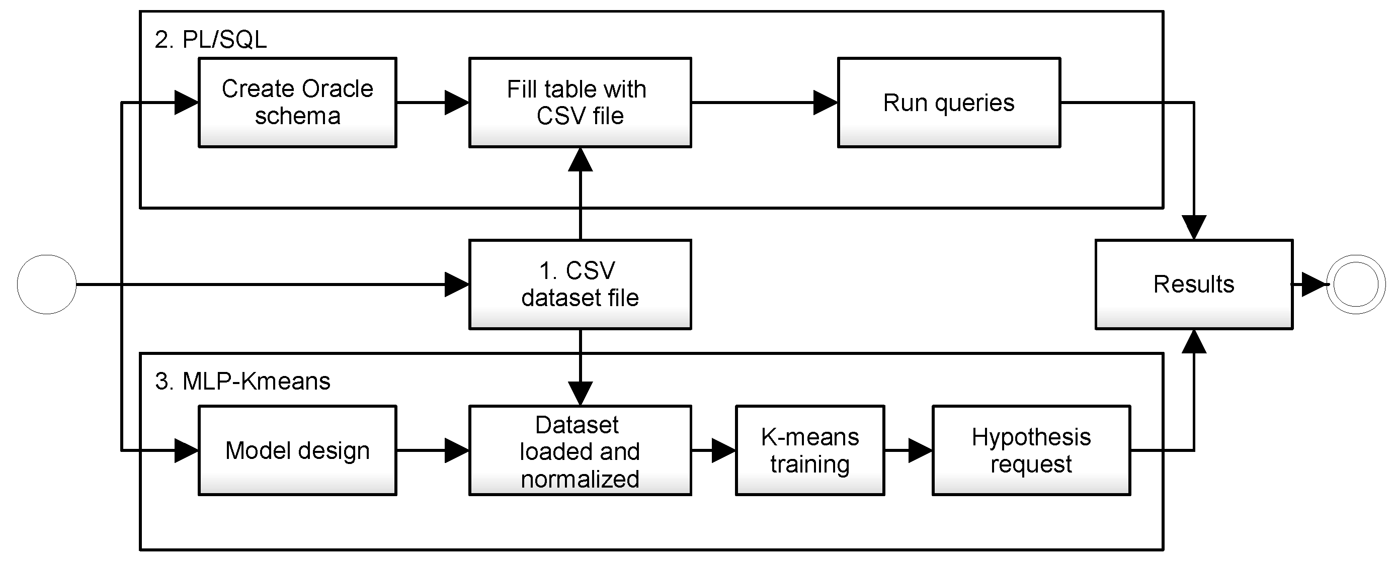
To illustrate the proposed methodology, Figure 1 presents a comparative scheme between the current PL/SQL query technique and the general MLP model, which includes training and clustering. While the PL/SQL data query is performed based on data indexation, the MLP model starts with a Kmeans model.
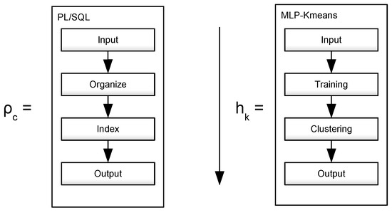
Figure 1.
Comparison between PL/SQL query process and MLP-Kmeans training.
2.1. Concerning the SQL Current Model
The process of assessing the quality of a query becomes exponentially challenging as query engines advance their techniques and optimization strategies, such as those used in an SQL Server [11]. Some modern databases are empowered with machine learning (ML), including SQL4ML, where users can write an objective function in a model similar to an SQL sentence. The model translates this into its equivalent in a TensorFlow graph, which can differentiate and optimize the model’s learning weights, achieving a 50% improvement in execution time and an 85% reduction in exported data [12]. Traditional database optimization techniques—such as cost estimation, joint arrangement selection, and mandate adjustment—often fail to meet high-performance requirements for large-scale database instances with diverse applications and users, especially in the cloud. Basic ML techniques can help alleviate these issues through historic data optimization learning [13].
In SQL, there are five instruction categories [14]: 1. Data Definition Language (DDL), which deals with table definitions, views, procedures, and functions—some instructions include CREATE TABLE, CREATE CONSTRAINT, DROP, and TRUNC; 2. Data Manipulation Language (DML), which focuses on data updates—instructions include INSERT, UPDATE, and DELETE; 3. Data Query Language (DQL), which manages data queries—the primary instruction is SELECT; 4. Data Control Language (DCL), which grants database privileges to users—the primary instruction is GRANT; and 5. Transaction Control Language (TCL), which assists with internal data administration, primarily data recovery—its primary instruction is ROLLBACK.
Sequences in SQL instructions are produced by application query generators like Relational OLAP, where report and analysis tasks are automated [15]. Formatting rules include identifying the necessity of indexes on specific columns if filters are included to optimize queries, avoiding unnecessary data usage and reducing execution time [16].
However, to the authors of [17], there are two main problems in optimizing queries:
- Computing the graph’s transitive closure.
- Obtaining the power of the adjacency matrix, evaluated using four graph types in efficient ascending order: binary trees, lists, cyclic graphs, and complete graphs.
Alternative data analysis techniques, such as Bayesian algorithms, offer solutions with advantages like handling parametric uncertainty in the study of irregular models [18]. In regression analysis involving predictors, variables are traced from the idea of sufficiency through subdivisions identified by categorical variables [19].
2.2. Concerning MLP-Kmeans
Generating symbolic rules is a natural way to determine inherent knowledge in interconnected models. When using MLP architecture-based rules with parallel axes positioned precisely, the values transformed into vectors can be effectively utilized in neural networks and support vector machines (SVMs) [20]. MLP and SVM algorithms, along with random forest and decision tree algorithms, have been employed to build predictive models for academic performance, including for students with disabilities, to enhance their college potential [21]. Query optimization is a sophisticated task, and validating its precision and effectiveness requires using relational algebra. This includes various classification and sorting techniques, such as the modular isomorphism problem, which assesses the performance of similar morphological groups and group classification by performance [22,23]. AI Models like deep learning (DL) models, convolutional neural networks (CNNs), and recurrent neural networks (RNNs) have been barely used in solving information security problems such as attack detection [24]. However, ref. [25], a relational and comparative analysis involving DL, the internet of things, and big data (BD), showed that current security solutions require updates similar to those already implemented with DL, which researchers and organizations have widely accepted.
The MLP algorithm is an artificial neural network (ANN) with at least three layers: input, hidden, and output [26]. It is commonly used due to its ability to model linear and non-linear estimative structures [27]. MLPs are also widely employed in classification tasks, capable of arbitrarily approximating complex functions to obtain results [28]. The two most frequently used activation functions in learning models are Sigmoid and ReLu [29]. The MLP has been applied effectively in treating and diagnosing chronic kidney disease, making it one of the most effective applications of an ANN [30].
Specifically, perceptron theory addresses how information is perceived and remembered, influencing recognition and behavior even after the input stops [31]. A perceptron is a weight optimization model that associates inputs (variables in a query) to desired results (the query) through an initial state (selected randomly) and an optimization process based on descending gradients, where the optimized variable is the response error compared to the desired outputs. On a broader scale, this also involves understanding the basic hardware for an ANN, projected on a larger scale depending on each neuron’s productivity at the execution level. This approach has shown favorable results in reconfiguring systems for integrated circuits, becoming an essential task [32].
The MLP architecture depends on the number of selected layers, hidden nodes in each layer, and the objective function. An improvement in this design is establishing control for each layer and removing those layers without connections, assigning a binary variable to each connection, which takes the value of 1 if the connection exists [33]. Learning models based on the standardization of non-linear processing elements have been designed to reduce the error cost function, which applies to predicting chaos in time series [34]. It is crucial to correctly select parameters to allow the model to adapt to observed data, appropriate layers, and weights. To address this, combinations of genetic algorithms and backpropagation have been proposed using one hidden layer [35].
3. Materials and Methods
This research was divided into three stages: the first one produces random data and stores it on a comma-separated value (CSV) file; the second one builds a schema on an standard Oracle ® database instance, where PL/SQL queries will be executed; and the third one constructs the MLP-Kmeans model, where training data will be used for a query, as described in Figure 2. On the PL/SQL side, queries were made through database indexation. On the MLP-Kmeans side, after training the dataset, the query, now termed a hypothesis, performed clustering operations.
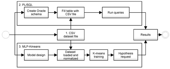
Figure 2.
Methodology for implementing PL/SQL and MLP models and results compilation.
3.1. Database and Schema Creation
The dataset simulates retail business operations and was created randomly, resulting in a CSV file with 306,849 records. The dataset includes the following fields:
- line: corresponds to the product line and is an Integer type.
- idproduct: corresponds to the product ID number and is an Integer type.
- amount: corresponds to the quantity sold and is a Double type.
All fields are numeric. Classification and clustering could be applied on fields line and idproduct.
In the sophisticated importation from text to SQL models (text-to-SQL), a binding a schema is considered easy, with errors mainly attributed to noise [36]. Systems that interpret human expressions with SQL instructions leverage exact lexical synchronization methods between keywords and schema elements. These methods face challenges in scenarios such as synonym substitution, where differences arise during synchronization [37]. To address this problem, schema preprocessing for tables and method redesign, consisting of schema expansion and schema pruning, have been incorporated [38].
3.2. PL/SQL Modeling
According to [39], database schema structures are sometimes dismissed either because they are too plain or because they are expected to be analyzed during the training or testing stages. For this work, a schema was built within an Oracle ® instance using DDL instructions: CREATE PROFILE..., CREATE TABLESPACE...and CREATE USER...
Data were imported from the CSV file into a table with the same name (ROWDATA) and identical data configuration. A test table was created from the same source by selecting one out of every 100 records, resulting in a table with 3069 records called ROWDATA_TEST.
PL/SQL Query Process
An essential part of software development is understanding how time is spent during program execution. However, more training is needed in using profilers, which often show bugs. These issues can be addressed by establishing a metaphorical relationship, where a bridge is built between statistical coverage and existing mutations [40]. Data profiling ranges from simple additions to complex statistics, aiding in understanding data. From a scientific perspective, it is crucial to know the data profile for manipulation and to update it according to new data schemas [41]. For this work, three queries were defined as follows:
- Line query. Request for line, product, and amount columns.
- Group query. Request for the sum of amount for each product.
- Total query. Request for the sum of all data amount.
3.3. MLP Modeling
Clustering modeling algorithms have been used to elaborate on the three kinds of queries, which, according to [42], are defined by an input and an output.
3.3.1. Input
The input is defined as a set of elements X and a distance function d as follows: , where is the set of non-negative real numbers, and when it is asymmetric, it satisfies for all subsets x that belong to X. In some cases, it requires a parameter k that determines the number of clusters, and according to the three queries established, we can have (line query), (group query), and (total query).
3.3.2. Output
The output is a domain partition of X where , producing the expression and that for every .
All groupings were taken from the sample X for each i cycle corresponding to the cluster defined by k, where the difference between epochs will produce an empty set. There is a link between clustering and optimal transport, equivalent to a restrained formulation where cluster dimensions are prescribed. This makes sense in a structure where each dataset class portion is known, but there is no information available at the individual level, aiming to establish concordant parameters [43].
In this work, the algorithm defined in [44] was used. Its mathematical representation is as follows:
where is the square sum of errors, C is a cluster, is the dataset instance that consists of N points, and is the cluster centroid in k, which is updated for each iteration according to
where is the total number of points in the kth cluster.
3.3.3. Hypothesis and Contribution
To address the proposed problem, the following corollary was derived from the theorem presented in Equation (1). For any query or hypothesis h, the search function is established as follows:
where is the hypothesis corresponding to the cluster index k, H is the set of all possible hypotheses according to the data availability, is the square sum of errors such that k is , and it exist in the dataset X, which constitutes the scientific proposition of this research.
3.3.4. Pseudocode
According to the last equation, the theorem’s executable application is set through the centroid closeness for each k measured using its Euclidean distance and established through the pseudocode of Algorithm 1.
| Algorithm 1 Centroid definition for three dimensions (x,y,z) and its euclidean distance |
|
3.3.5. Parameterization
According to the three hypothesis requested, cluster parameterization is defined as follows:
- 1.
- Line query: when each element is a cluster or the size of the cluster is equal to the size of elements.
- 2.
- Group query: when each k cluster is the sum of all i clusters with the same requested parameter.
- 3.
- Total query: when there is only one cluster.
Under this proposal, 306,850 registers were analyzed with three points, A, B, and C, each one with three coordinates: x, y, and z. Although the algorithm was designed for objects in three dimensional calculations (coordinates), in this case, Euclidean and centroid distances were measured only using the x coordinate, corresponding to the point and data: A (line), B (idproduct), and C (amount). The coordinates y and z remained with their initial 0 value.
3.3.6. Training Using Kmeans
Kmeans is used for data classification into categories or clusters, referred to as k, based on the proximities of the Euclidean distances from their centroids. In this study, the training process began by selecting k values randomly from the dataset. Each record was then assigned to the nearest k, based on the Euclidean distance. After the initial assignment, the centroids of each k were iteratively adjusted over n epochs to achieve the optimal Cartesian position.
3.3.7. Parameters for MLP-Kmeans Model
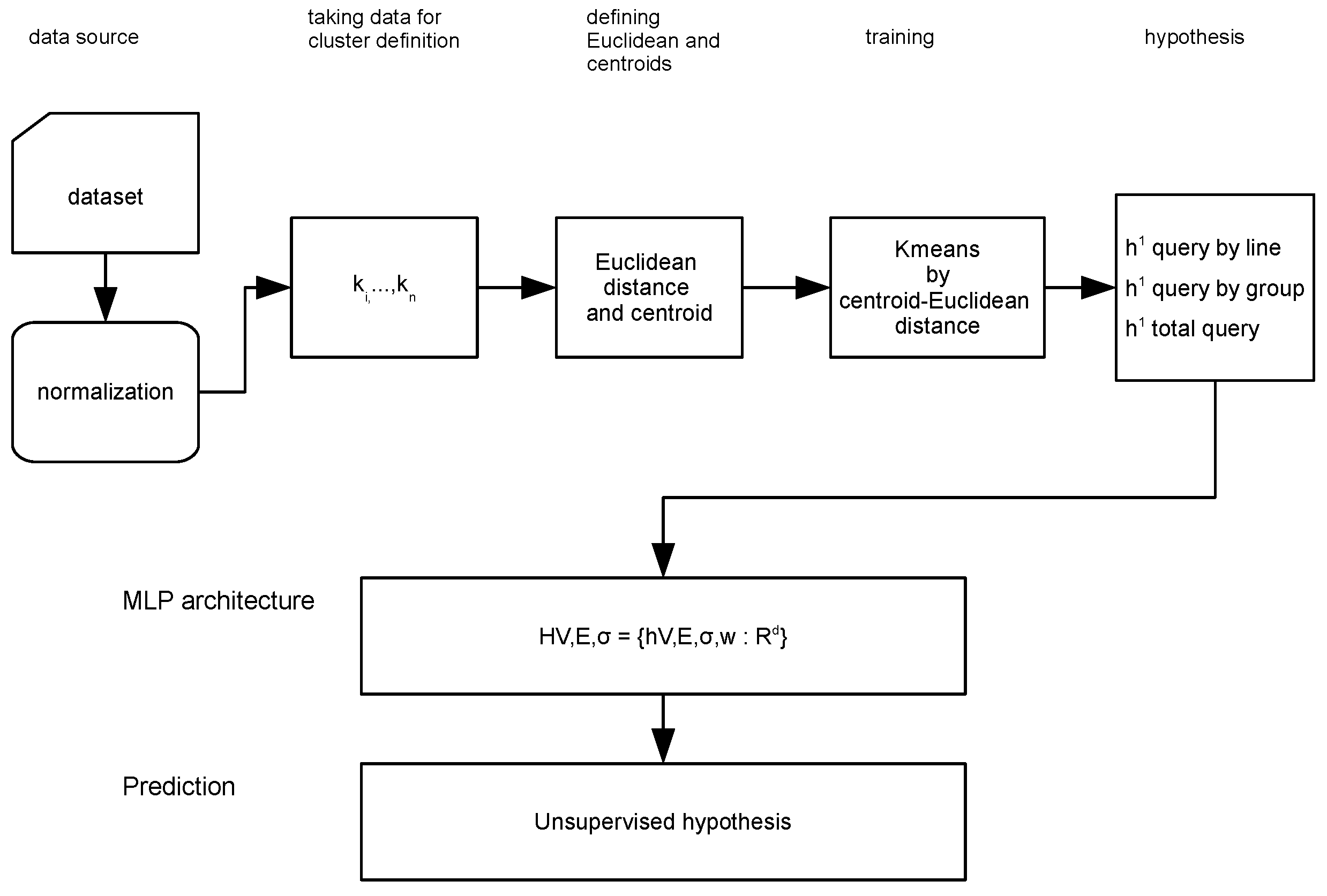
The MLP architecture is defined by the triplet , where V represents the number of layers, E denotes the boundaries that correspond to the weights, and is the activation function. With the Kmeans component integrated, the entire model is depicted in Figure 3.
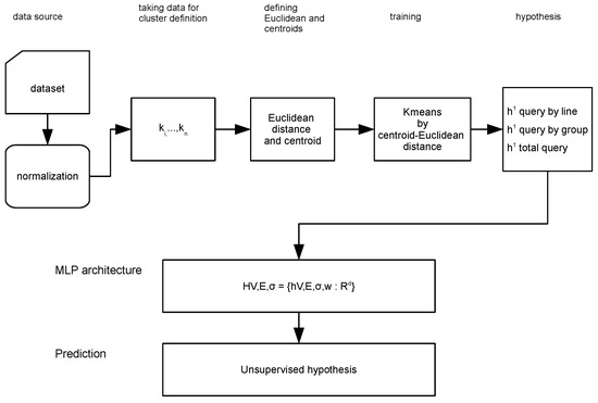
Figure 3.
Integrated MLP-Kmeans model architecture.
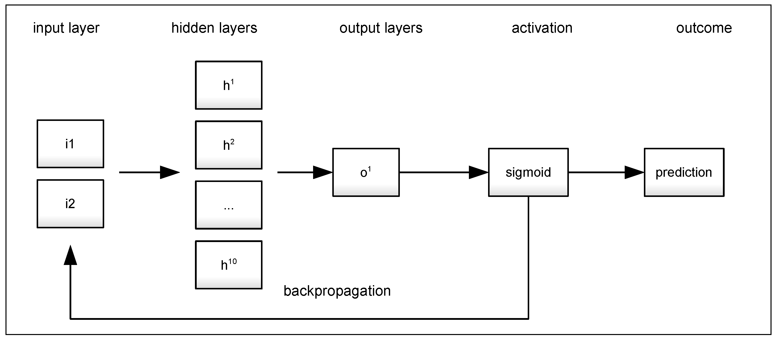
The connection between the two models was established through the group query hypothesis provided by Kmeans, and the interpretability of the MLP model drives to the amount and categorization of the clusters that will be set for analysis in the Kmeans process. The proposed methodology helps as a hash table estimated to improve the computation and resources to minimize the response time in querying a data base. The layers V are defined as follows: is the input layer with 2 neurons, corresponding to the k values provided by Kmeans. is the hidden layer with 10 neurons, and is the output layer with 1 neuron, corresponding to the specific prediction or hypothesis. The value of corresponds to the sigmoid function. In this work, each neuron requires 3 input values , corresponding to the values. The inner product <> is calculated, the activation value is defined, and the weight value is transferred to the successive layers, as illustrated in Figure 4 and the algorithm pseudocode in Algorithm 2.
| Algorithm 2 Layer definition for MLP model linked with Kmeans model |
|
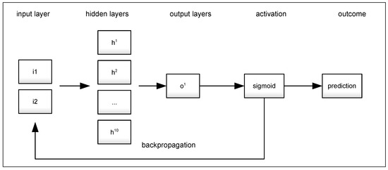
Figure 4.
MLP definition.
4. Results
The training dataset was rewritten from NoSQL by eliminating unnecessary data, removing columns with non-numeric values, and normalizing the remaining data to standardize different categories and visualize query results. For the MLP-Kmeans model, the design incorporated a clustering perspective with corresponding parameters attached to each aleatory category and hypothesis. Finally, a comparative analysis was conducted between both models to discuss the results and establish conclusions.
4.1. PL/SQL Results
At the end of the research activity, the results obtained for each case are the following.
4.1.1. Line Query
Table 1 displays the query line by line without category definitions. This would be the equivalent in Kmeans to k = 0, or the lack of k, showing all data and the total amount of the run-time consumption.

Table 1.
Line query.
4.1.2. Group or Category Query
Table 2 presents the data grouped by categories (lines), and the count of each idproduct by line. In Kmeans terms, this is equivalent to a hypothesis k. The third column shows the sum of the amount value for each line and the total process time consumption.

Table 2.
Group query.
4.1.3. Total Query
When the query is applied for one category without using filters, the total calculation k value is 0, and there is no need to deploy data. The result is the total sum of 306,849 lines in 0.013 s. Group queries are the slowest due to the grouping operation.
4.2. MLP Results
The outcome of the MLP-Kmeans model is presented as follows, starting with the Kmeans analysis.
4.2.1. Line Query
For this query, the parameters were set as and . The result was less than 0.009 s.
4.2.2. Group Query
Table 3 represents the classification of randomly selected categories, with parameters set as and . The records (X values) were grouped according to the Euclidean distance concerning each k.

Table 3.
Clusters selected randomly from the dataset.
From the last table, training consisted of adjusting the centroid to the most efficient point from the Euclidean distance concerning each data centroid of its particular category k, resulting in Table 4.

Table 4.
Trained clusters (10 epochs).
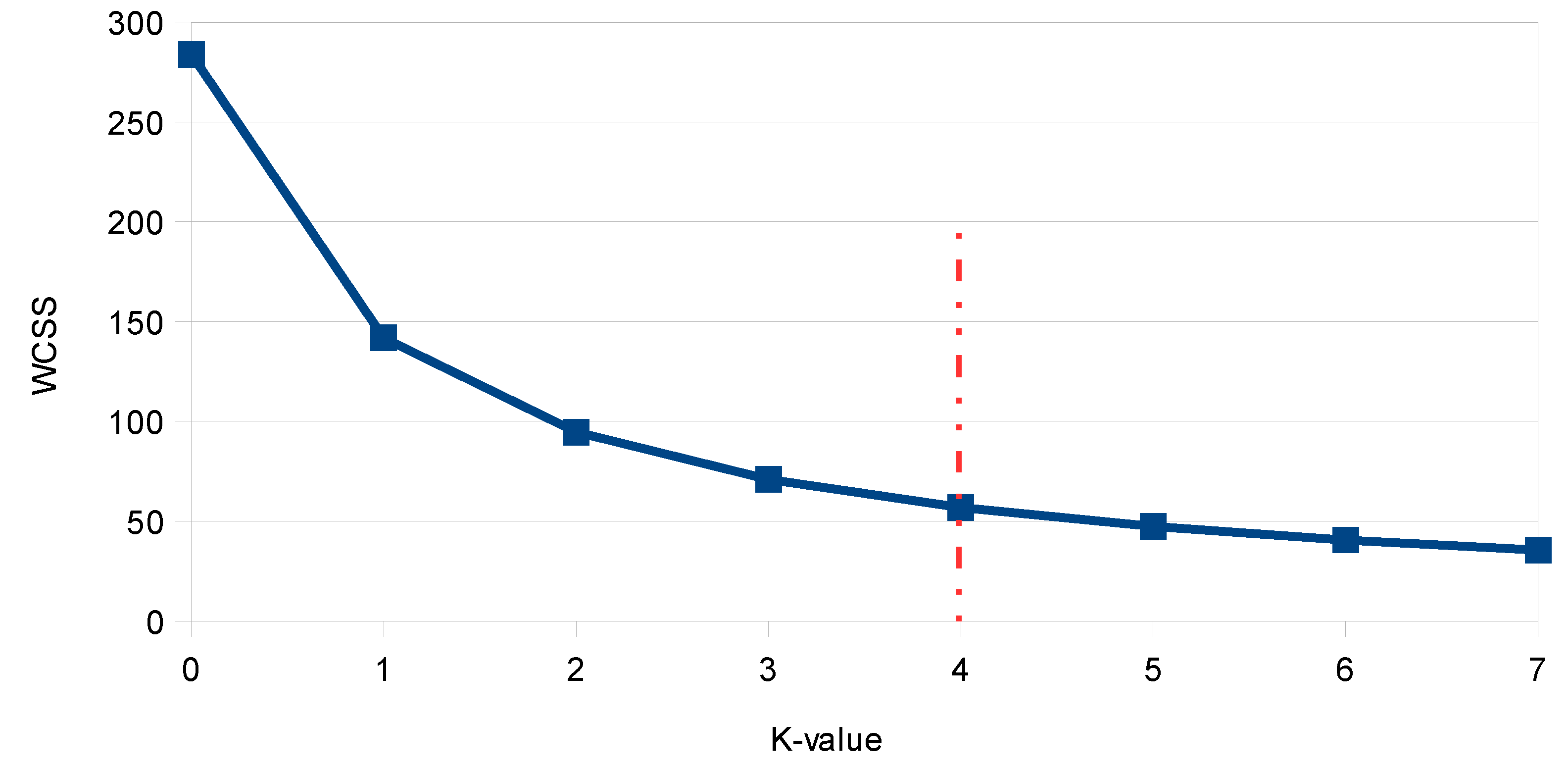
The Elbow Method was used to find the optimal value of k, where the sum of the square distance between one cluster and the centroid cluster (within-cluster sum of square, WCSS) was calculated. For comparative reasons, Figure 5 and Figure 6 are shown for cases where and .

Figure 5.
Optimal K value through WCSS (or Elbow) method for .
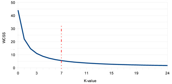
Figure 6.
Optimal K value through WCSS (or Elbow) method for .
4.2.3. Total Query
The parameters were established as and .
4.2.4. Summary
In summary, the previous queries defined three hypotheses, and their efficiency relationship is shown in Table 5. It is important to note that all queries were made after data loading and normalization, causing a 0-time consumption in line query. Also, the execution was not presented in the compiler console.

Table 5.
Solved hypothesis.
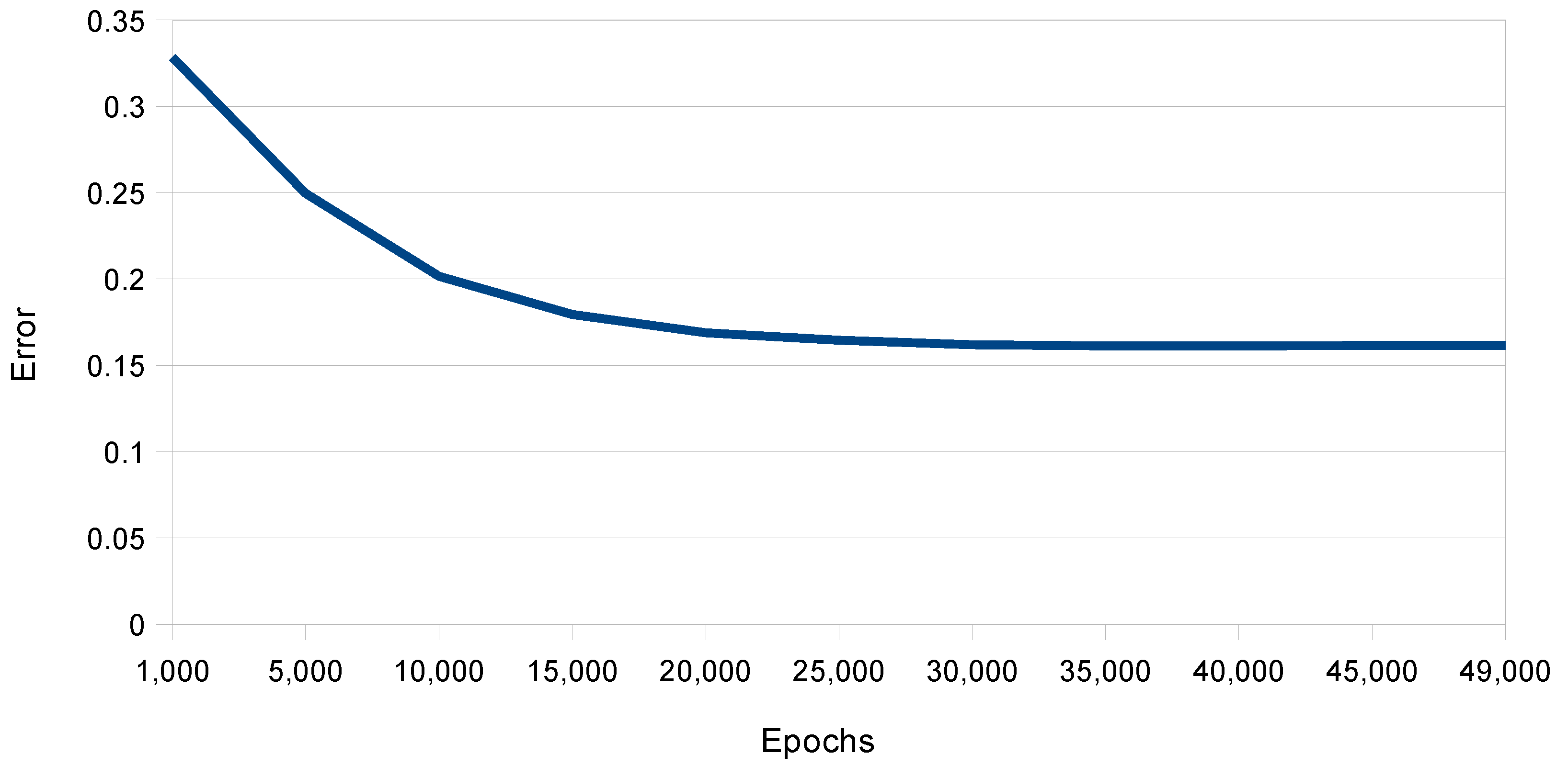
The model was run multiple times with different parameters to enhance the data analysis. The indicators obtained from the model execution after 50,000 epochs were the Mean Absolute Error (MAE) = 0.16, Mean Square Error (MSE) = 0.03, Root Mean Square Error (RMSE) = 0.18,, and Coefficient of Determination () = 0.29. The learning curve shown in Figure 7 indicates a consistent trend from the 20,000 epochs, so extending it further is unnecessary due to the emergence of overfitting.
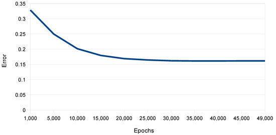
Figure 7.
Learning curve for 50,000 epochs.
4.3. Comparative Analysis between PL/SQL and MLP-Kmeans
Once the experimentation was realized, a comparative analysis between the two models was conducted. Table 6 summarizes the results, indicating the increase in time consumption in the MLP-Kmeans trained model concerning the PL/SQL model.

Table 6.
Comparative efficiency between PL/SQL and MLP-Kmeans (seconds).
5. Discussion
In the case of the first hypothesis, the line query where , it was not necessary to perform training because the number of clusters was the same as the number of data lines, so the data retrieval was immediate. In the case of the group query, , where n is the number of clusters selected, the level of training defines the efficiency: time is proportionally direct to the value of k. In the case of the total query, where , the data were obtained after grouping some randomly selected centroids. In the end, training consumption is represented by the model’s friction and fatigue: friction for the k number and fatigue for the quantity defined in the parameters. Once the model was trained, efficiency depended on the hardware resources. Table 7 shows some other models used in other research to define the optimal k value.

Table 7.
Quality comparison with other similar models.
6. Conclusions
When comparing different methodologies, it becomes evident that training can lead to increased fatigue and consume a lot of time when dealing with database queries. Additionally, the complexity of using a neural network can produce more accurate results compared to using simple PL/SQL instructions in the testing scenario. This will be particularly significant in the future for specific problem-solving scenarios, such as intelligent environments characterized by prescriptive control achieved through self-programming processes, resulting in holistic functionality, for which this work should be extended to [50]. For instance, generative AI for tendency queries is required to analyze trends on social networks to group frequencies and data types and determine real proclivity for productive user entailment. This can be achieved using centroids.
The following contributions were made in this work:
- The proposal for a corollary from the basic Kmeans theorem.
- The definition of a centroid training model for Euclidean distance for n coordinates.
- An MLP-Kmeans model for classification.
Author Contributions
Conceptualization, V.H.S.-B., A.M.H.-N. and J.M.Á.-A.; methodology, V.H.S.-B., J.M.Á.-A. and H.J.-H.; software, V.H.S.-B.; validation, A.M.H.-N., D.M.C.-E., J.R.-R. and H.J.-H.; formal analysis, A.M.H.-N., J.R.-R. and H.J.-H.; investigation, V.H.S.-B.; writing—review and editing, V.H.S.-B., J.R.-R. and J.M.Á.-A.; visualization, V.H.S.-B.; supervision, A.M.H.-N. and D.M.C.-E.; project administration, A.M.H.-N. and D.M.C.-E. All authors have read and agreed to the published version of the manuscript.
Funding
This research received no external funding.
Data Availability Statement
https://github.com/victorhugosilvablancas/mlp_vs_plsql (accessed on 27 March 2024).
Acknowledgments
We sincerely thank the Consejo Nacional de Humanidades Ciencias y Tecnología (CONAHCYT) for the invaluable support provided through the doctoral scholarship.
Conflicts of Interest
The authors declare no conflicts of interest.
Abbreviations
The following abbreviations are used in this manuscript:
| AI | Artificial Intelligence |
| ANN | Artificial Neural Network |
| BD | Big Data |
| BP | Backpropagation |
| CC | Cloud Computing |
| CNN | Convolutional Neural Networks |
| DCL | Data Control Language |
| DDL | Data Definition Language |
| DML | Data Manipulation Language |
| DQL | Data Query Language |
| Kmeans | Kmeans clustering |
| MLP | Multilayer Perceptron Neural Network |
| PL | Procedural Language |
| RNN | Recurrent Neural Network |
| SQL | Structured Query Language |
| TCL | Transaction Control Language |
References
- Wang, T.; Zhou, J.; Chen, X.; Wang, G.; Liu, A.; Liu, Y. A Three-Layer Privacy Preserving Cloud Storage Scheme Based on Computational Intelligence in Fog Computing. IEEE Trans. Emerg. Top. Comput. Intell. 2018, 2, 3–12. [Google Scholar] [CrossRef]
- Ning, Z.; Dong, P.; Wang, X.; Wang, S.; Hu, X.; Guo, S.; Qiu, T.; Hu, B.; Kwok, R.Y.K. Distributed and Dynamic Service Placement in Pervasive Edge Computing Networks. IEEE Trans. Parallel Distrib. Syst. 2021, 32, 1277–1292. [Google Scholar] [CrossRef]
- Ren, Y.; Leng, Y.; Qi, J.; Sharma, P.K.; Wang, J.; Almakhadmeh, Z.; Tolba, A. Multiple cloud storage mechanism based on blockchain in smart homes. Future Gener. Comput. Syst. 2021, 115, 304–313. [Google Scholar] [CrossRef]
- Li, W.; Xu, H.; Li, H.; Yang, Y.; Sharma, P.K.; Wang, J.; Singh, S. Complexity and Algorithms for Superposed Data Uploading Problem in Networks With Smart Devices. IEEE Internet Things J. 2020, 7, 5882–5891. [Google Scholar] [CrossRef]
- Ashraf, D.; Ella, H.A.; Mohamed, E.; Kumar, S.A.; Khan, M. The impact of the hybrid platform of internet of things and cloud computing on healthcare systems: Opportunities, challenges, and open problems. J. Ambient Intell. Humaniz. Comput. 2019, 10, 4151–4166. [Google Scholar] [CrossRef]
- Wu, K.; Di, D.; Li, W.; Cui, W. Design and implementation of a general SQL parser. J. Phys. Conf. Ser. 2021, 2010, 012093. [Google Scholar] [CrossRef]
- Zhao, J.; Liu, C. Design and Implementation of SQL Injection Vulnerability Scanning Tool. J. Phys. Conf. Ser. 2020, 1575, 012094. [Google Scholar] [CrossRef]
- Kumar, P.R.; Raj, P.H.; Jelciana, P. Exploring Data Security Issues and Solutions in Cloud Computing. Procedia Comput. Sci. 2018, 125, 691–697. [Google Scholar] [CrossRef]
- Zhang, J.; Chen, B.; Zhao, Y.; Cheng, X.; Hu, F. Data Security and Privacy-Preserving in Edge Computing Paradigm: Survey and Open Issues. IEEE Access 2018, 6, 18209–18237. [Google Scholar] [CrossRef]
- Zhang, X.; Chen, X. Data Security Sharing and Storage Based on a Consortium Blockchain in a Vehicular Ad-hoc Network. IEEE Access 2019, 7, 58241–58254. [Google Scholar] [CrossRef]
- Giakoumakis, L.; Galindo-Legaria, C.A. Testing SQL Servers Query Optimizer: Challenges, Techniques and Experiences. IEEE Data Eng. Bull. 2008, 31, 36–43. [Google Scholar]
- Makrynioti, N.; Ley-Wild, R.; Vassalos, V. Machine learning in SQL by translation to TensorFlow. In Proceedings of the DEEM 21: Proceedings of the Fifth Workshop on Data Management for End-To-End, Virtual Event, China, 20–25 June 2021; Volume 2, pp. 1–11. [Google Scholar] [CrossRef]
- Li, G.; Zhoy, X.; Cao, L. Machine Learning for Databases. In Proceedings of the First International Conference on AI-ML-Systems, Bangalore, India, 21–24 October 2021. [Google Scholar] [CrossRef]
- McLaughlin, M.; Harper, J. PL/SQL Programming Workbook; McGrawHill: New York, NY, USA, 2010. [Google Scholar]
- Kraft, T.; Schwarz, H.; Rantzau, R.; Mitschang, B. Coarse-Grained Optimization: Techniques for Rewriting SQL Statement Sequences. In Proceedings of the 2003 VLDB Conference, Berlin, Germany, 9–12 September 2003; Morgan Kaufmann: Burlington, MA, USA, 2003; pp. 488–499. [Google Scholar] [CrossRef]
- Hayath, T.; Usman, K.; Mohammed, S.; Dadapeer. An Overview of SQL Optimization Techniques for Enhanced Query Performance. In Proceedings of the 2023 International Conference on Distributed Computing and Electrical Circuits and Electronics (ICDCECE), Ballar, India, 29–30 April 2023; pp. 1–5. [Google Scholar] [CrossRef]
- Carlos, O. Optimization of Linear Recursive Queries in SQL. IEEE Trans. Knowl. Data Eng. 2010, 22, 264–277. [Google Scholar] [CrossRef]
- Moins, T.; Arbel, J.; Girard, S.; Dutfoy, A. Reparameterization of extreme value framework for improved Bayesian workflow. Comput. Stat. Data Anal. 2023, 187, 107807. [Google Scholar] [CrossRef]
- Ke, C.; Yang, W.; Yuan, Q.; Li, L. Partial sufficient variable screening with categorical controls. Comput. Stat. Data Anal. 2023, 187, 107784. [Google Scholar] [CrossRef]
- Bologna, G.; Hayashi, Y. A Rule Extraction Study from SVM on Sentiment Analysis. Big Data Cogn. Comput. 2018, 2, 6. [Google Scholar] [CrossRef]
- Huynh-Cam, T.-T.; Chen, L.-S.; Huynh, K.-V. Learning Performance of International Students and Students with Disabilities: Early Prediction and Feature Selection through Educational Data Mining. Big Data Cogn. Comput. 2022, 6, 94. [Google Scholar] [CrossRef]
- Margolis, L.; Moede, T. The Modular Isomorphism Problem for small groups—Revisiting Eicks algorithm. J. Comput. Algebra 2022, 2, 100001. [Google Scholar] [CrossRef]
- Dolorfino, M.; Martin, L.; Slonim, Z.; Sun, Y.; Yang, Y. Classifying solvable primitive permutation groups of low rank. J. Comput. Algebra 2023, 5, 100005. [Google Scholar] [CrossRef]
- Jiang, F.; Fu, Y.; Gupta, B.B.; Liang, Y.; Rho, S.; Lou, F.; Meng, F.; Tian, Z. Deep Learning Based Multi-Channel Intelligent Attack Detection for Data Security. IEEE Trans. Sustain. Comput. 2020, 5, 204–212. [Google Scholar] [CrossRef]
- Amanullah, M.A.; Habeeb, R.A.A.; Nasaruddin, F.H.; Gani, A.; Ahmed, E.; Nainar, A.S.M.; Akim, N.M.; Imran, M. Deep learning and big data technologies for IoT security. Comput. Commun. 2020, 151, 495–517. [Google Scholar] [CrossRef]
- Subasi, A. Chapter 3 - Machine learning techniques. In Practical Machine Learning for Data Analysis Using Python; Academic Press: Cambridge, MA, USA, 2020; pp. 91–202. [Google Scholar] [CrossRef]
- Aydin, N.; Sahin, N.; Deveci, M.; Pamucar, D. Prediction of financial distress of companies with artificial neural networks and decision trees models. Mach. Learn. Appl. 2022, 10, 100432. [Google Scholar] [CrossRef]
- Chen, Z.; Czarnuch, S.; Dove, E.; Astell, A. Automated recognition of individual performers from de-identified video sequences. Mach. Learn. Appl. 2023, 11, 100450. [Google Scholar] [CrossRef]
- Sudqi Khater, B.; Abdul Wahab, A.W.; Idris, M.Y.; Abdulla Hussain, M.; Ahmed Ibrahim, A. A Lightweight Perceptron-Based Intrusion Detection System for Fog Computing. Appl. Sci. 2019, 9, 178. [Google Scholar] [CrossRef]
- Qezelbash-Chamak, J.; Badamchizadeh, S.; Eshghi, K.; Asadi, Y. A survey of machine learning in kidney disease diagnosis. Mach. Learn. Appl. 2022, 10, 100418. [Google Scholar] [CrossRef]
- Rosenblatt, F. The perceptron: A probabilistic model for information storage and organization in the brain. Psychol. Rev. 1958, 65, 386–408. [Google Scholar] [CrossRef]
- Rana, A.; Singh Rawat, A.; Bijalwan, A.; Bahuguna, H. Application of Multi Layer (Perceptron) Artificial Neural Network in the Diagnosis System: A Systematic Review. In Proceedings of the 2018 International Conference on Research in Intelligent and Computing in Engineering (RICE), San Salvador, El Salvador, 22–24 August 2018; pp. 1–6. [Google Scholar] [CrossRef]
- Ramchoun, H.; Ghanou, Y.; Ettaouil, M.; Janati, I.; Mohammed, A. Multilayer perceptron: Architecture optimization and training. Int. J. Interact. Multimed. Artif. Intell. 2016, 4, 26–30. [Google Scholar] [CrossRef]
- Ergezinger, S.; Thomsen, E. An accelerated learning algorithm for multilayer perceptrons: Optimization layer by layer. IEEE Trans. Neural Netw. 1995, 6, 31–42. [Google Scholar] [CrossRef]
- Castillo, P.; Merelo, J.; Prieto, A.; Rivas, V.; Romero, G. G-Prop: Global optimization of multilayer perceptrons using GAs. Neurocomputing 2000, 35, 149–163. [Google Scholar] [CrossRef]
- Lei, W.; Wang, W.; Ma, Z.; Gan, T.; Lu, W.; Kan, M.-Y.; Chua, T.-S. Re-examining the Role of Schema Linking in Text-to-SQL. In Proceedings of the 2020 Conference on Empirical Methods in Natural Language Processing (EMNLP), Online, 16–20 November 2020. [Google Scholar] [CrossRef]
- Liu, A.; Hu, X.; Lin, L.; Wen, L. Semantic Enhanced Text-to-SQL Parsing via Iteratively Learning Schema Linking Graph. In Proceedings of the 28th ACM SIGKDD Conference on Knowledge Discovery and Data Mining, Washington, DC, USA, 14–18 August 2022. [Google Scholar] [CrossRef]
- Chen, Z.; Yu, S.; Adam, P.; Antonios, P.E. Bridging the Generalization Gap in Text-to-SQL Parsing with Schema Expansion. In Proceedings of the 60th Annual Meeting of the Association for Computational Linguistics, Dublin, Ireland, 22–27 May 2022. [Google Scholar] [CrossRef]
- Ben, B.; Matt, G.; Jonathan, B. Representing Schema Structure with Graph Neural Networks for Text-to-SQL Parsing. In Proceedings of the 57th Annual Meeting of the Association for Computational Linguistics, Florence, Italy, 28 July–2 August 2019. [Google Scholar] [CrossRef]
- Yang, Y.; Jiang, Y.; Zuo, Z.; Wang, Y.; Sun, H.; Lu, H.; Zhou, Y.; Xu, B. Automatic Self-Validation for Code Coverage Profilers. In Proceedings of the International Conference on Automated Software Engineering (ASE), San Diego, CA, USA, 11–15 November 2019; pp. 79–90. [Google Scholar] [CrossRef]
- Colleoni, C.J.; Juliana, D.; Rafael, B.; Duncan, R. New Trends in Big Data Profiling. Intell. Comput. 2022, 1, 808–825. [Google Scholar] [CrossRef]
- Shalev-Shwartz, S.; Ben-David, S. Understanding Machine Learning From Theory to Algorithms; Cambridge University Press: Cambridge, UK, 2014. [Google Scholar]
- Genevay, A.; Dulac-Arnold, G.; Vert, J.-P. Differentiable Deep Clustering with Cluster Size Constraints. arXiv 2019, arXiv:1910.09036. [Google Scholar]
- Arvanitidis, A.I.; Bargiotas, D.; Daskalopulu, A.; Kontogiannis, D.; Panapakidis, I.P.; Tsoukalas, L.H. Clustering Informed MLP Models for Fast and Accurate Short-Term Load Forecasting. Energies 2022, 15, 1295. [Google Scholar] [CrossRef]
- Sinaga, K.P.; Yang, M.-S. Unsupervised K-Means Clustering Algorithm. IEEE Access 2020, 8, 80716–80727. [Google Scholar] [CrossRef]
- Fard, M.M.; Thonet, T.; Gaussier, E. Deep k-Means: Jointly clustering with k-Means and learning representations. Pattern Recognit. Lett. 2020, 138, 185–192. [Google Scholar] [CrossRef]
- Benaimeche, M.A.; Yvonnet, J.; Bary, B.; He, Q.-C. A k-means clustering machine learning-based multiscale method for anelastic heterogeneous structures with internal variables. Int. J. Numer. Methods Eng. 2022, 123, 2012–2041. [Google Scholar] [CrossRef]
- Song, Y.; Kim, H.-J.; Lee, H.-J.; Chang, J.-W. A Parallel Privacy-Preserving k-Means Clustering Algorithm for Encrypted Databases in Cloud Computing. Appl. Sci. 2024, 14, 835. [Google Scholar] [CrossRef]
- George, S.; Seles, J.K.S.; Brindha, D.; Jebaseeli, T.J.; Vemulapalli, L. Geopositional Data Analysis Using Clustering Techniques to Assist Occupants in a Specific City. Eng. Proc. 2023, 59, 8. [Google Scholar] [CrossRef]
- Augusto, J.C.; Callaghan, V.; Cook, D.; Kameas, A.; Satoh, I. Intelligent Environments: A manifesto. Hum.-Centric Comput. Inf. Sci. 2013, 3, 12. [Google Scholar] [CrossRef]
Disclaimer/Publisher’s Note: The statements, opinions and data contained in all publications are solely those of the individual author(s) and contributor(s) and not of MDPI and/or the editor(s). MDPI and/or the editor(s) disclaim responsibility for any injury to people or property resulting from any ideas, methods, instructions or products referred to in the content. |
© 2024 by the authors. Licensee MDPI, Basel, Switzerland. This article is an open access article distributed under the terms and conditions of the Creative Commons Attribution (CC BY) license (https://creativecommons.org/licenses/by/4.0/).


