Abstract
Permanent Magnet Synchronous Motors (PMSMs) with high energy efficiency, reliable performance, and a relatively simple structure are widely utilised in various applications. In this paper, a suboptimal controller is proposed for PMSMs without sensors based on the state-dependent Riccati equation (SDRE) technique combined with customised impulsive observers (IOs). Here, the SDRE technique facilitates a pseudo-linearised display of the motor with state-dependent coefficients (SDCs) while preserving all its nonlinear features. Considering the risk of non-available/non-measurable states in the motor due to sensor and instrumentation costs, the SDRE is combined with IOs to estimate the PMSM speed and position states. Customised IOs are proven to be capable of obtaining quality, continuous estimates of the motor states despite the discrete format of the output signals. The simulation results in this work illustrate an accurate state estimation and control mechanism for the speed of the PMSM in the presence of load torque disturbances and reference speed changes. It is clearly shown that the SDRE-IO design is superior compared to the most popular existing regulators in the literature for sensorless speed control.
1. Introduction
Permanent Magnet Synchronous Motors (PMSMs) have advantages such as constant speed, an adjustable power factor, high efficiency, field winding elimination, DC power supply rejection, Joule loss deletion in excitation circuits, omission in brushes and slip rings, a short radial length, and easy maintenance [1,2,3,4,5]. They have simple configurations and easy-to-understand operation mechanisms which make them ideal to be used as actuators in many applications [6,7].
The control of PMSMs has progressed very well in the last few decades. Examples include works such as [8], where Nonlinear Model Predictive Speed Controllers (NMPSCs) are proposed to predict and control the positions and speed at each sampling period through the variable forecast horizon. In [9], to estimate and control the rotor speed and position, an Extended Kalman Filter (EKF) is designed for a sensor-free vector control drive. In [10,11], linear model prediction controllers (MPCs) with the addition of least mean square (LMS) identification strategies and online parameter detection are presented for permanent magnet synchronous generators (PMSGs). In [12], a Robust Adaptive Backstepping Control (RABC) is suggested for High-Speed Permanent Magnet Synchronous Motors (HSPMSM). In [13], a Sliding Mode Observer (SMO) and Sliding Mode Control (SMC) are, respectively, employed to estimate and control the motor speed, torque, and current with third-degree harmonic current. In [14], a model reference adaptive system (MRAS) for estimating and controlling the velocity in internal PMSMs with bandwidth modulation is offered. Furthermore, in [15], an MRAS controller is utilised for sensorless speed control. The authors used the pseudo-linearisation technique and produced state-dependent matrices. Then, the state-dependent matrices were applied to an MRAS mechanism. It should be noted that only the pseudo-linearisation concept was used, and the Riccati equation technique was not investigated in [15]. Moreover, an adaptive, interconnected observer was suggested in order to estimate the speed. In [16], a robust adaptive observer-based approach for the sensorless speed control of PMSMs is studied to estimate the rotor shaft speed and position. In [17], an Adaptive Nonlinear Continuous Observer (ANCO) is used to estimate the self-induction coefficient, stator resistance, rotor velocity/position, and load torque by using the current measurements for the PMSM. In [18], adaptive fuzzy RST digital control (AFRSTD), digital control, and fuzzy digital RST control are generated for a PMSM system. In [19], a Sliding Mode focused on an Extended State Observer (SMESO) and Fast Terminal Sliding Mode Control (FTSMC) is recommended to develop disturbance elimination capacity and increase the dynamic performance of PMSM drive systems.
Reviewing the literature as summarised above reveals that most of the controllers and observers designed for PMSMs have been based on approaches that depend on linear or linearised models. These approaches, although simple, are not ideal for dealing with the inherent nonlinearities of a PMSM. Conventional linearisation methods such as Jacobian approximations do not preserve critical information about the nonlinear mechanisms and are usually time-invariant to reduce the controller design efforts. However, these aspects all reduce the control performance. In the same context, Linear Quadratic Regulators (LQRs) have been shown to perform very well for many linear systems. Therefore, numerous efforts have been made to expand them to nonlinear dynamical systems. The introduction of the state-dependent Riccati equation (SDRE) [20,21,22,23] technique was an effort to fulfil this desire. The SDRE technique is a state-dependent control method based on a pseudo-linearisation display which produces a optimal plan for the cost function of a suboptimal solution [20,21,22,23]. In the SDRE technique, the nonlinear system is transformed into a pseudo-linearised matrix depending on states without any approximation. This pseudo-linearisation representation might not be unique, and there might be countless versions that would make the degrees of freedom of the controller infinite. This is one of the aspects that requires research for its application in different systems.
The SDRE technique has been applied in many applications, such as robotics, navigation systems, Unmanned Aerial Vehicles (UAVs), submarines, Heating Ventilation and Air Conditioning Systems (HVACs), healthcare, and power systems [21,22,23]. In [24], a suboptimal SMC was obtained from a mix of the SDRE and SMC for a class of nonlinear closed-loop systems for the Scout robot. In [25], an SDRE controller was designed for UAVs using the Artificial Potential Field (APF) approach. In [26], the nonlinear SDRE was applied for the fault-tolerant control of a DC micro-grid (MG) in the power system.
On the other hand, the SDREs face challenges regarding access to the system’s states for feedback design. Here, state observers can provide a solution. In [27], the SDRE method is utilised for both control and observation purposes for an Air Handling Unit (AHU) system. The Riccati equation is solved at every sample time, and a suboptimal control law and an estimated state vector are produced based on its solution. It should be noted that the SDRE observer needs continuous data from output sensors at each sample time. In this regard, impulsive systems and observers are well suited for simulating real-world systems in which internal states change instantaneously. Compared to classical continuous and discrete systems, impulsive systems can contain sudden, abrupt, and intermittent changes at variable time intervals [28,29]. In such a mechanism, an impulse could model the sudden change that happens in the system state. The time intervals between these impulses can be fixed or variable with time, known or unknown, and deterministic or stochastic. In [30], an impulsive observer (IO) is introduced based on state-dependent matrices for nonlinear time-delay systems. Furthermore, an adaptive IO (AIO) is suggested for a class of nonlinear time-delay systems with unknown parameters in [31]. Moreover, in [32], an AIO is investigated based on the feasibility of a centralisation perspective for a class of uncertain nonlinear systems.
Based on the literature review summarised and the challenges listed above, in this paper, a state-dependent, centred pseudo-linearisation representation is combined with an impulsive observer to not only estimate motor speed/position in a so-called “sensorless” scheme but also to control these parameters. The proposed observer can provide continuous estimates of the output states of the system, even in the presence of discrete output measurements. Through this approach, by utilising a pseudo-linearisation display instead of linearisation, not only is the design of a linear control scheme facilitated, but also all the nonlinear specifications of the system are preserved along with an accurate estimate of the states.
It should be mentioned that in [27], the authors used an SDRE controller and SDRE observer for an AHU system. The SDRE observer used continuous output signals to estimate the states, and its structure is of the Luenberger type but with state-dependent matrices. Both controller and observer gains are obtained by solving the SDRE at every sample time. In the present paper, the SDRE controller is used with an observer state-dependent impulsive observer for the PMSM when no speed sensors are available. This observer only utilises the output signal at impulse times and does not require continuously estimated states (between the impulses). In [15], the authors used an MRAS to control an IPMSM. The purpose of the mentioned paper was to use the pseudo-linearisation presentation in the structure of the MRAS controller. To estimate the speed, stator resistance, winding inductance, and torque load, an augmented adaptive interconnected observer (AAIO) was used with a similar structure in [33].
In [30], the basic structure of the state-dependent impulsive observer is introduced for nonlinear time-delay systems. The Congo Ebola disease is addressed and presented as a case study without any input control signal criteria. The combination of the SDRE and an impulsive observer was introduced for the first time by the authors of [34] for a manipulator robot case study. The major difference between the present paper and this previous one is that each joint of the manipulator arm was assumed to have a control actuator, and there were the same number of output and control input signals in this system. Thus, the input matrix was an orthogonal one. Unlike the previous case study, the PMSM system in the present paper has only states that are measurable. Therefore, for the speed and position signals, no direct control is available. Also, here, it is assumed that the angles are measured and available only in impulse time stamps, and only angular velocities are estimated by the observer, i.e., there is no access to physical measurements. Addressing this state access problem while there is a nonlinear dependency between the outputs and speed signals is the key challenge addressed in this work. This challenge is addressed through the following:
- Developing a pseudo-linearised representation of the PMSM system.
- Designing a controller for optimal tracking of the PMSM’s reference speed with high accuracy and a quick speed without a speed sensor.
- Estimating motor speed in a sensorless framework.
- Addressing the challenge of disturbances during the course of the control.
- Maintaining the function of estimation and speed control during all times of sampling and not just at the impulse sample times.
- Quantifying the effects of impulse intervals (the sample rate) and load torque.
The simulated examples in this work demonstrate the performance of the controlled system despite the changes in the reference speed and load torque and the variable sample rates. To show the superiority of the proposed estimation and control approach, the results are compared with the linear control approach of LQRs. It is worth noting that the PMSM here is only considered as a case study, and the proposed work has the potential to be applied to systems with similar challenges and requirements without a loss in generalisability.
Given the introduction and motivation for this work given above, the rest of the paper is organised as follows: Section 2 is dedicated to the state-dependent Riccati equation principles, and Section 3 summarises the fundamentals of the impulsive state estimator. Section 4 includes the main results and the proposed work; the stability theorems and the proofs are given in this section. Section 5 is dedicated to the PMSM control case study, with simulations and visualisations given in Section 6; this section includes a comprehensive discussion of the results, the sensitivity analysis, and practical considerations as well. Comparisons are also included in this section. The last section includes the conclusion and potential future work.
2. State-Dependent Riccati Equation
In the SDRE method, the nonlinear system is first transformed into a pseudo-linearisation form without any approximation, and then the benefits of the linear representation are used to design the controller, observer, or any nonlinear filters. Its ability to be implemented in a wide range of nonlinear systems, the existence of a methodical process for the transformation, and the possibility of obtaining optimal solutions for control purposes are among the advantages of the SDRE technique [21,22,23].
The dynamics of a nonlinear system are considered as follows [21]:
where , , and are, respectively, the states, control, and output vectors of the system. and are the nonlinear functions here. The pseudo-linearised display of the system (1) is as follows:
, , and are the system’s state-dependent coefficient matrices, inputs, and outputs, respectively. To track the reference path of the system, the cost function with the SDRE’s infinite time horizon is defined as follows:
where the weight coefficients and are state-dependent [24] and can determine state or input preferences. The control input to minimise the cost function (4) is calculated as follows [20]:
such that and are the solutions to the Riccati equation in the form of (5):
where is the solution to the following algebraic equation:
In the process presented above, optimal tracking can be achieved without worrying about the rank reduction in the controllability and observability matrices.
3. Impulsive Observer
In this section, it is described how the state observer is designed to estimate the states of the system. Through this framework, the controller can perform based on the estimated states. Impulsive systems have two continuous and discrete dynamic behaviours. The continuous dynamic behaviours are described by differential equations that are continuous in time, describing the intervals between impulses. However, the discontinuous dynamic behaviour is described by differential equations that denote the impulse moments when system states abruptly change. According to these features, impulsive systems are very suitable for describing real-world variable processes in which system states change instantaneously at certain points in time. Impulsive dynamic systems can be seen as a subset or class of hybrid systems with precipitate jumps. There is a main continuous or discrete dynamic in impulsive systems, in which moments also occur between impulses and change the states of the system. The time interval between these impulses can be fixed or variable with time, known or unknown, and deterministic or stochastic.
In general, for a nonlinear system, the system is denoted as in Equation (7) [28]:
with as the continuous state vector and as the time variable. With, and as nonlinear functions with appropriate dimensions, the state variable jumps can be expressed as in discrete intervals of , where . is also known as the Impulsive Differential Equation (IDE). There are two main approaches to studying stability issues in impulsive systems. The classical approach is based on the positive definite Lyapunov function, with a negative derivative for non-impulsive systems. It should be noted that most of the existing articles have used the classical perspective to examine the stability of a system or its observer. Unlike non-impulsive systems, impulsive systems can have a positive derivative at some point in time but have a descending trend overall [28].
A system with impulsive equations is defined as follows:
where and are continuous, and is non-descending. Also, the following equations are established:
Hypothesis 1.
It is assumed that , , and for all with .
Therefore, the obvious response of the main system and the comparison system is in . The theorem of the comparison system is presented as Theorem 1.
Theorem 1.
The conditions are assumed to be as follows:
- -
- , , in , and .
- -
- There is a , so and for all , and in , .
- -
- on when .
Moreover, the stability characteristics of the obvious solution to the comparison system will result in the stability of the main system [28].
Outcome 1.
Suppose when and . The origin of the main system will be asymptotically stable if the following conditions are met:
State-Dependent Impulsive Observer
A state-dependent impulsive observer (SDIO) is suggested as follows:
where and are the estimated state and output vectors, respectively. is the jump vector of the estimated states. The observer gain is , which is also determined according to the closed-loop stability theorem [29].
4. Main Design: SDRE Controller Based on State-Dependent Impulsive Observer
The impulsive observer is assumed to be state-dependent (11). The control input when using the state-dependent Riccati controller is as follows:
Hypothesis 2.
The following Lipshitz conditions are assumed to be valid for the system:
where and are constant and positive.
Theorem 2.
The proposed state-dependent impulsive observer’s estimation error for the SDRE controller is , which will converge to zero asymptotically when the following assumptions and conditions are met:
where , , , and are the design parameters, and .
Proof of Theorem 2.
The SDRE closed-loop system is written as follows:
where
and . It can also be written for the observer in :
Therefore, the dynamics of the estimation error in
are rewritten as follows:
where
and . In ,
The positive definite Lyapunov function is introduced as follows:
where is an alternating matrix in , and and are defined as symmetric, positive definite matrices.
So, the derivative of the Lyapunov function in the time interval is equal to
Using the Yang inequality [30], the result is as follows:
And, according to Hypothesis 2, the following result is obtained:
Hence, the derivative of Lyapunov’s function will be taken as follows:
By applying to (28), the following result is obtained:
which can be written as follows:
If , , and the following conditions are satisfied by the LMIs (14), as well as the definition of , the first condition of the comparison system theorem is established as follows:
In , the Lyapunov function is presented as follows:
This is the case if the following condition is met:
which is the same condition for the LMI (16) as and .
Therefore, the second condition of the comparison system theorem is established. □
According to the third condition, the upper limit of the impact distance is obtained as follows:
5. Case Study: Permanent Magnet Synchronous Motor
The dynamic model of the permanent magnet synchronous motor used in this paper on the axis is as follows [35]:
where and are the currents and and are the voltages of the and axes, respectively. is the stator resistance. and are, respectively, the inductances of the winding on the and axes. and are the magnetic flux of the permanent magnet and the mechanical speed of the motor, respectively. and are the angular position of the rotor and the moment of inertia. is the coefficient of friction. is the number of poles, and is the load torque. Table 1 presents the values of the engine parameters according to [35]. The pseudo-linearised representation of the PMSM is obtained as follows:
where is the state vector, is the input vector, and is the output vector. The advantage of this presentation is that it is both controllable and observable.

Table 1.
The PMSM’s parameters [35].
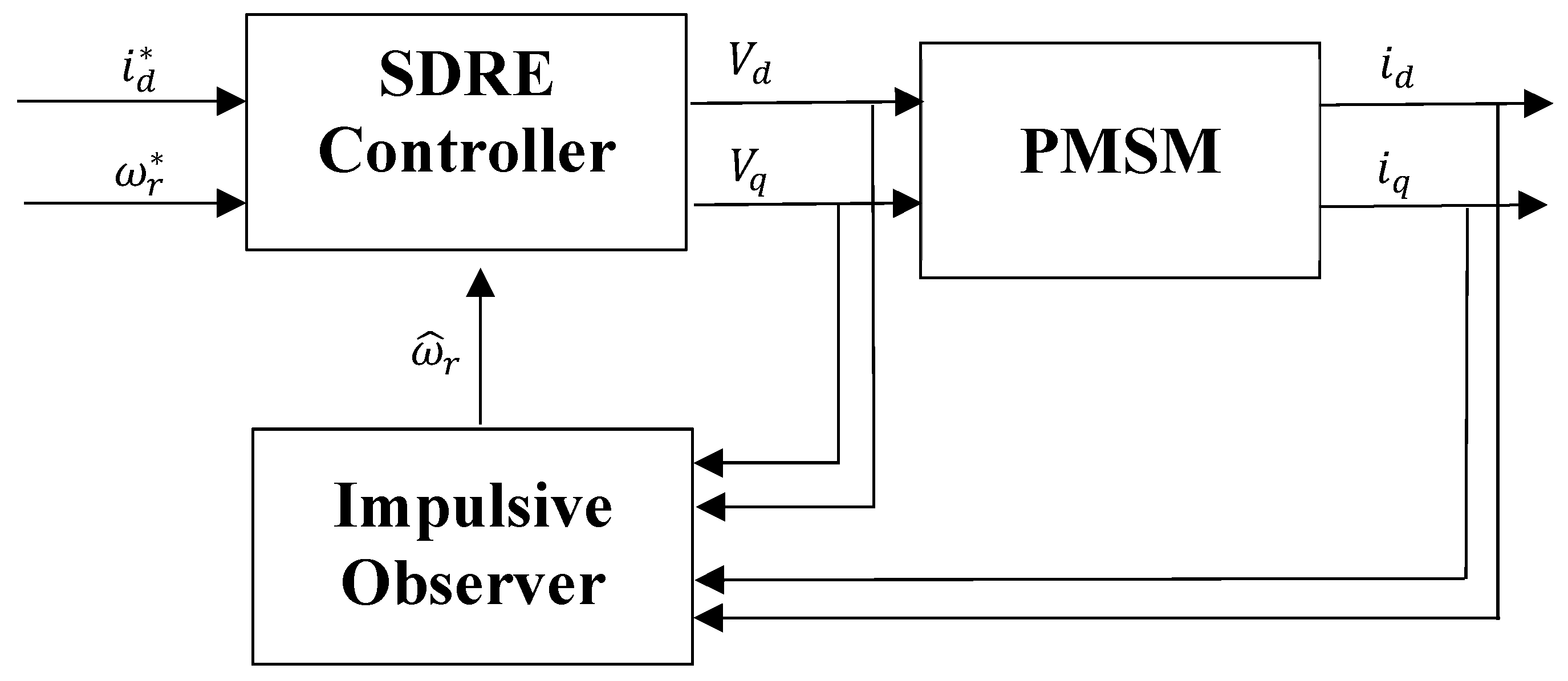
An overview of the control, speed estimation, and identification of the synchronous motor’s parameters is shown in Figure 1. In this block diagram, the voltage in the d–q plane is applied to the motor, and the currents are captured as the response. These current values are not necessarily available at each sample point, but to reduce the cost of measurements, they are assumed to be available only for a few time stamps. The impulse observer receives the current and voltage values and estimates the motor speed for all of the time stamps. This speed is then used as an input to the SDRE controller for tracking purposes. Here signals with * reference to the setpoint of the system.
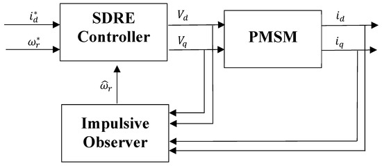
Figure 1.
Block control diagram of the proposed method.
6. Simulation Results and Discussions
6.1. The Main Simulation Results
The design parameters are considered as follows:
The initial conditions of the states and their estimations are as follows:
Also, the desired values of the speed and current on the d-axis are assumed to be zero. According to the values of the design parameters, the maximum distance between impulses is calculated as s. The sampling time s, and the interval between impulses is also assumed to be s, which means that an output is available every five sampling times. The tracking error is defined as and the estimation error is called as .
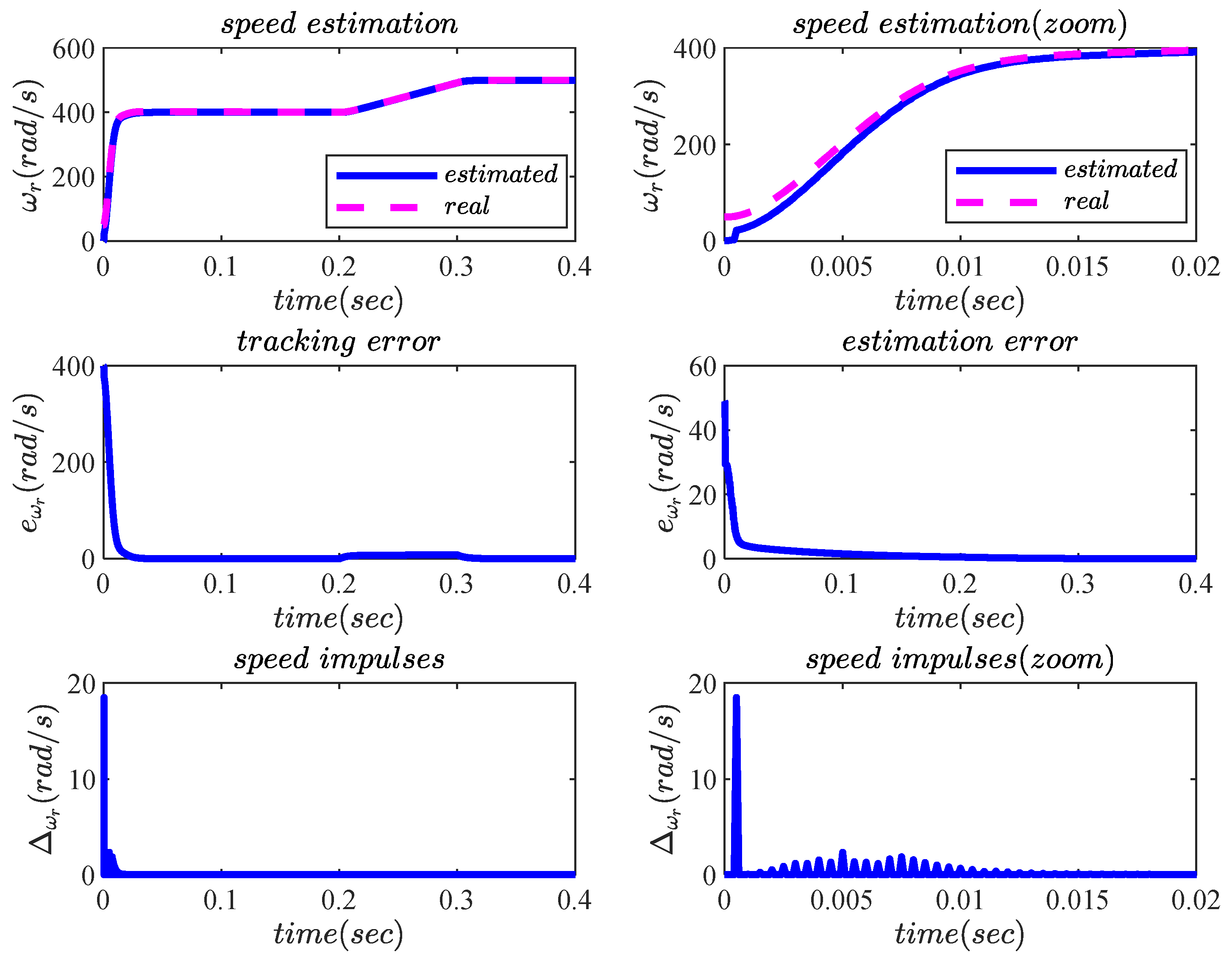
The results were simulated by MATLAB 2023b software with an ASUS laptop (Ausu Laptop Model: K556CPU COREi7/7500u, RAM DDR4, Graphic GFORCE 940MX). These results are displayed in Figure 2 for the speed tracking error, the speed estimation error, and the estimated speed jumps (speed impulses). The figures on the top row are the tracking performance and its zoomed-in version. It is very clear that the reference speed was successfully tracked after only the first 0.02 s. The figures in the second row demonstrate the tracking errors, which are very small after convergence happens. According to the results, it is clear that the proposed observer can estimate the motor speed very well. The proposed controller also tracks reference paths with appropriate accuracy. At first, it is seen that, despite the error between the actual and estimated values, these jumps have a greater amplitude, which gradually decreases.
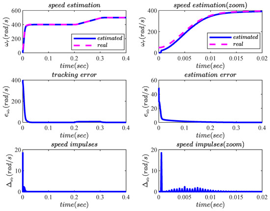
Figure 2.
Speed profiles of the PMSM, the state estimation, the tracking error, and the speed impulses, together with the zoomed-in areas.
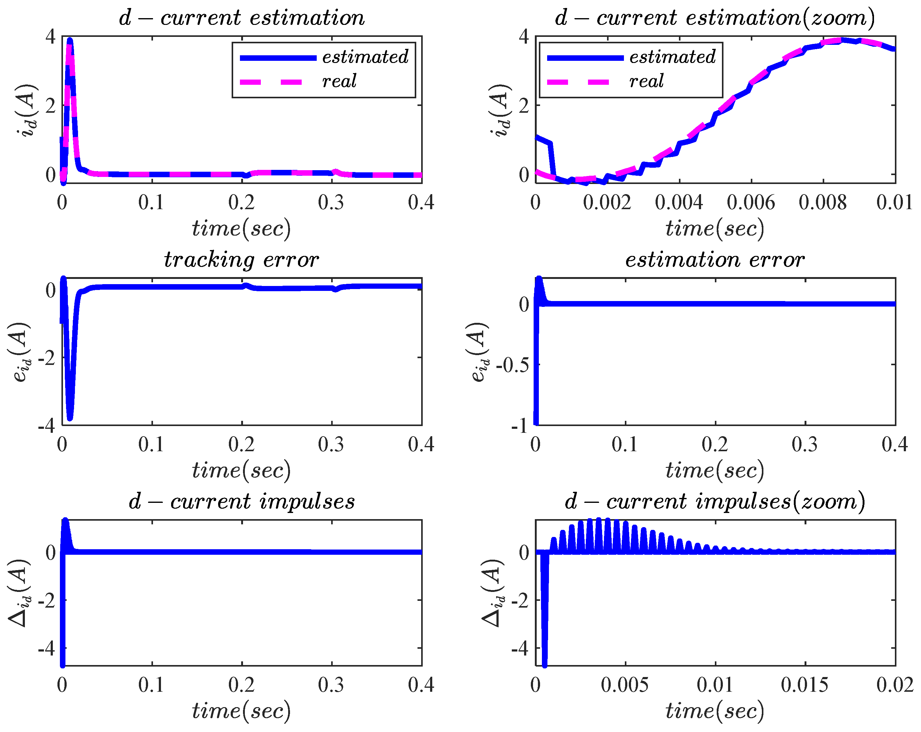
Further results are plotted in Figure 3 to show the d-current estimation, the d-current tracking error, the d-current estimation error, and the estimated d-current jumps (d-current impulses).
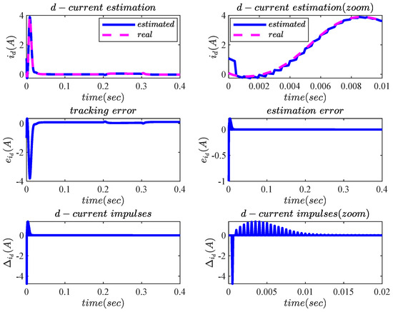
Figure 3.
Current on the d-axis of the PMSM, the estimated states, the errors, and the impulses.
Figure 4 illustrates the q-current estimation, the q-current estimation error, and the estimated q-current jumps (q-current impulses). Eventually, as the signal converges to the true value, the jump amplitude also becomes zero.
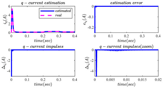
Figure 4.
Current on the q-axis of the PMSM, the estimated states, the errors, and the impulses.
The control inputs are shown in Figure 5. As can be seen, all inputs and their changes are smooth and slow. The allowed range for the input control signals was between −250 and +250, so it is clear that the signals are within the prescribed range. Therefore, these inputs can be implemented in practice. Generally, in the proposed method, the control signals can be forced to stay within a range by tuning the controller’s parameters. Also, by making a trade-off between the performance and the control input variations, a design that can be implemented in real applications can be achieved.

Figure 5.
Voltage along the d-axis and q-axis of the PMSM, along with the d–q axis.
The observer gains are also plotted in Figure 6, which are obtained at any time by solving the LMIs of Theorem 2. Obviously, the gains remain unchanged after the conversion.
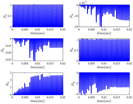
Figure 6.
Impulsive observer gains over the course of estimation and control.
6.2. The Effect of Impulse Intervals
To show the effects of impulse intervals on the estimation error of the states by the proposed observer, the two criteria of the normalised mean square error (NMSE) and the correlation coefficient (CC) were used. These two criteria can be calculated as follows:
where is the error of the state. The NMSE metric shows the strength of the estimation and the correlation coefficient of the similarity of the real and estimated states. If the two signals are completely similar, the correlation coefficient is 1, and if they are completely different, the correlation coefficient is −1.
Table 2 shows that the accuracy of the estimation decreases with increasing impulse intervals, although the values are still acceptable up to the maximum impulse intervals determined by the proposed Theorem 2. In the last column, where the impulse interval is selected above the maximum value, a high error is witnessed, and the similarity between the actual and estimated signals is reduced.

Table 2.
Summary of the impulse interval effect.
6.3. The Effect of Load Torque
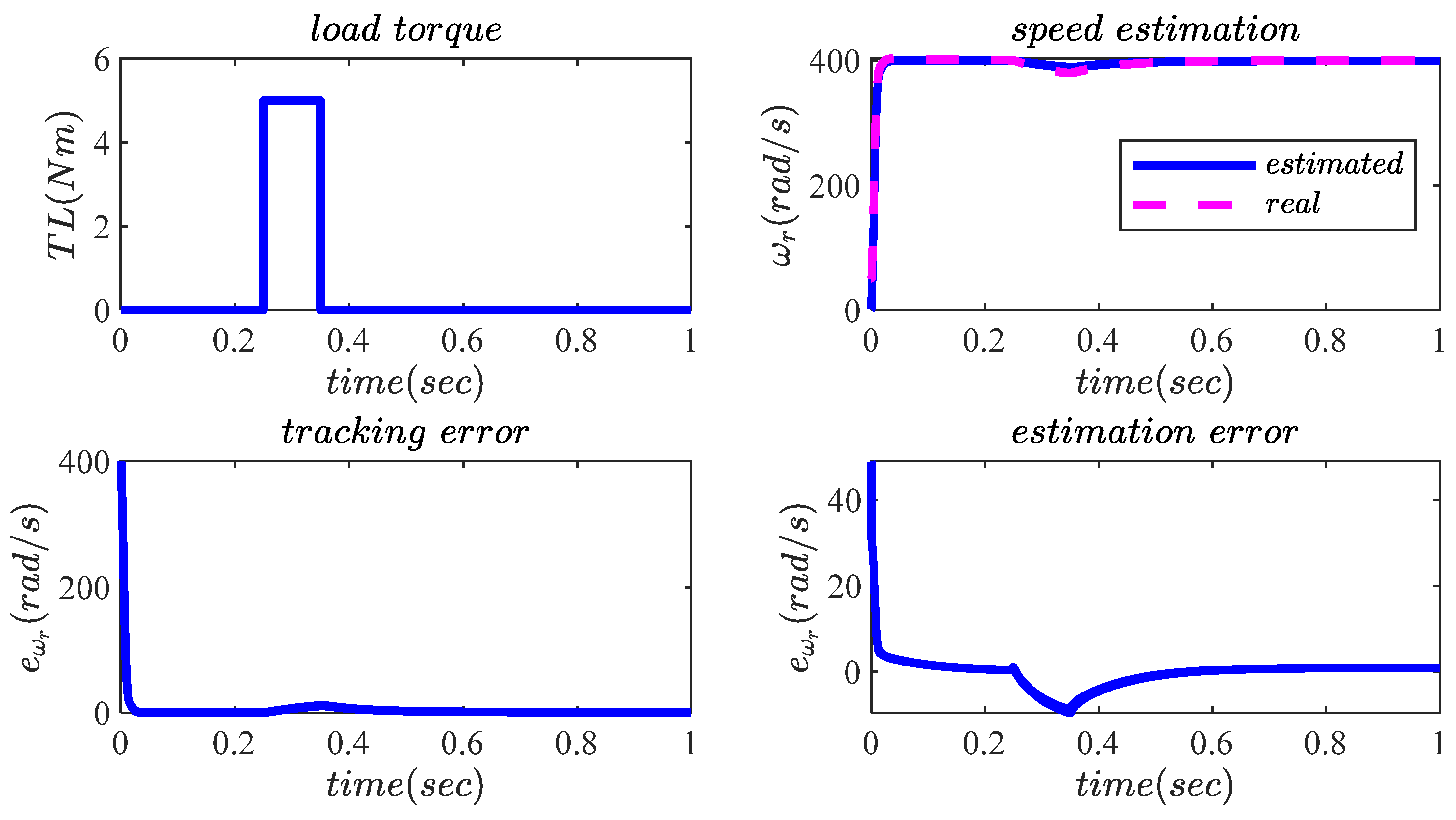
In this section, to investigate the effect of the load torque as a disturbance to the performance of the closed-loop system, a load torque of 5 Nm at an equilibrium point from to per second is applied to the motor. The load torque impulsive observer gains, speed tracking and estimation with load torque, speed tracking error with load torque, and speed estimation error with load torque are plotted in Figure 7.
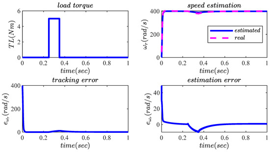
Figure 7.
Load torque impulsive observer gains, speed tracking and estimation with load torque, speed tracking error with load torque, and speed estimation error with load torque.
According to the results, it is clear that despite the load torque acting on the system as a disturbance, the performance of the proposed controller and observer in tracking reference paths and estimating the states is satisfactory. The tracking error is directly related to increasing or decreasing load torque amplitude. It is worth noting that the load torque was considered such that a change in the speed or current response is visible. Robust approaches should be used if there is more disturbance or higher accuracy is required.
6.4. Comparisons
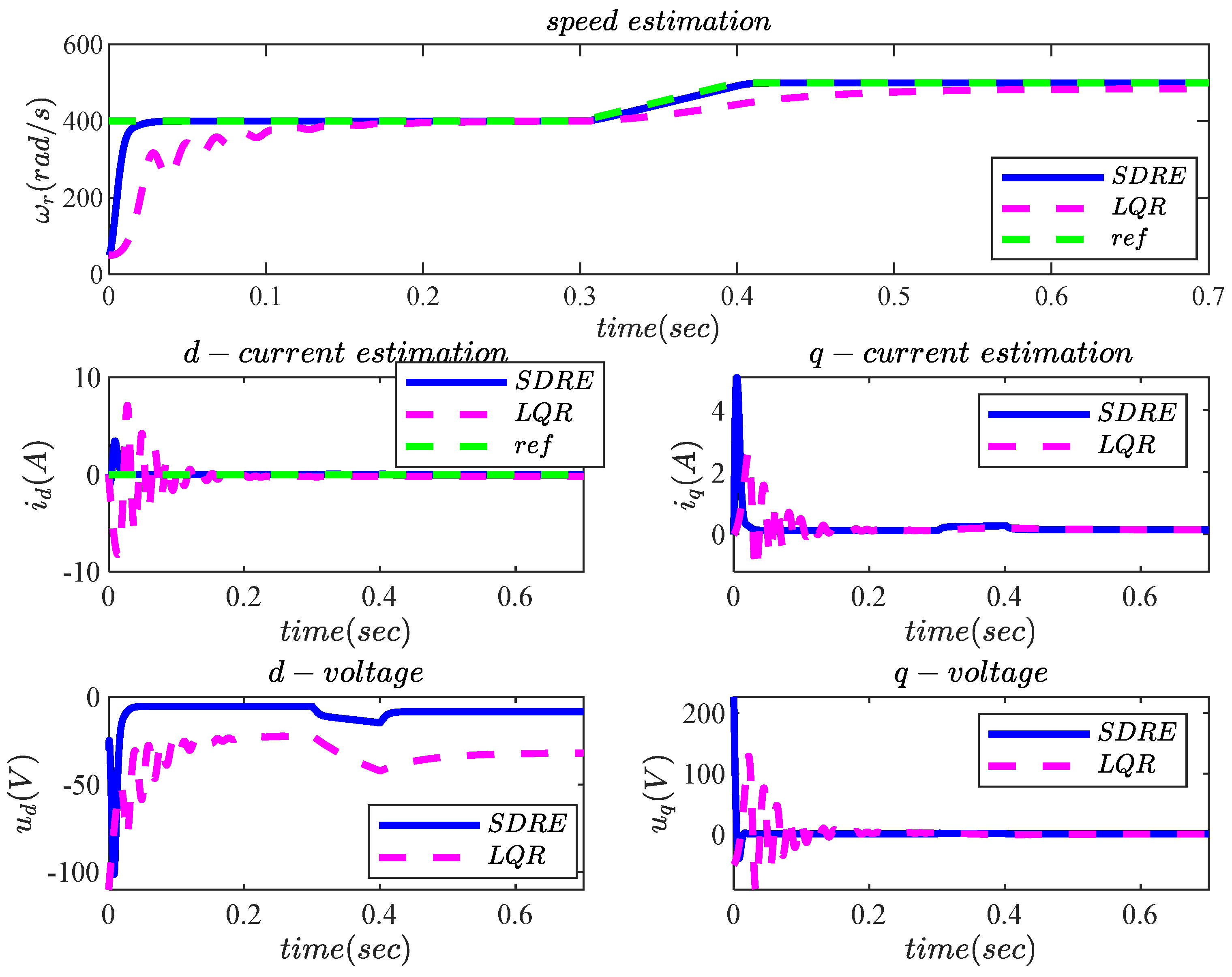
In this section, a comparison between the SDRE and LQR optimal controllers is provided. In this comparison, the SDRE controller examines the system nonlinearly, and the LQR, which is a linearised version, examines the system linearly. This comparison shows the better performance of the SDRE method. In the SDRE approach, a pseudo-linearisation matrix and SDC are generated, which will preserve the nonlinear properties of the system, whereas in the LQR version, the system is first linearised around the equilibrium point. So, this linearisation cannot include nonlinear features of the system and eliminates them. Hence, the system does not have a nonlinear nature and will have the same system matrices at all times. Meanwhile, the system matrices in the SDRE controller update their state-dependent system matrices at each sampling time. This solves the state-dependent Riccati equation for each time sample. But in LQRs, the Riccati equation is checked only once. The linearisation of the motor equations around the equilibrium point is performed using the Jacobian method as follows:
The weighting coefficients and are considered to be the same in both the LQR and SDRE methods, and the calculation of these coefficients is arbitrary. The response of the algebraic Riccati equation for the matrices (39) and the LQR state feedback gain is obtained as follows:
The following figures show the outputs and states of the SDRE and LQR controllers. Both controllers assume that all states are available, and they track both paths optimally. Figure 8 displays the speed estimation, currents (d-axis and q-axis), and voltages (d-axis and q-axis). It is clear that the SDRE controller performs much better than the LQR, especially when changing the equilibrium point. Because the LQR controller is linearised around the equilibrium point, by changing the equilibrium point, the linearisation accuracy is significantly reduced. Furthermore, Table 3 shows a numerical comparison between the proposed method and the LQR. The numerical results verified the efficiency of the proposed framework compared to the LQR technique in varying the reference speed.
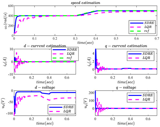
Figure 8.
Comparison of PMSM parameters between the SDRE and the LQR.

Table 3.
Summary of the comparison between the proposed method and the LQR.
As Table 3 shows, for both cases, the distance between the impulses (where the output signals become available) is 0.005 s. In both cases, a similar impulse observer was designed. However, the LQR performs more weakly compared to the SRDE controller. All the performance measures of the NMSE, c c1, c c2, and c c3, which are the normalised mean squared errors and correlation coefficients across both the d and q axes, are lower for the LQR compared to the SDRE. Based on the performance metrics, this superiority is due to the SDRE being able to take care of the system’s intrinsic nonlinearities, especially when the working point changes during tracking.
7. Conclusions
In this article, an observer-based suboptimal controller for the PMSM according to the SDRE controller and impulsive observer approaches was applied, and a pseudo-linearised representation and SDRE strategy procedure were presented. Moreover, a mathematical formulation of the impulsive state observer was presented. The proposed SDRE technique guarantees the tracking of reference paths with acceptable accuracy and speed. Despite the change in the reference speed, the performance of the closed-loop system was maintained, and the reference paths were well tracked. The results illustrate that despite the load torque, the performance of the system decreases to some extent, but it is still acceptable. A comparison was applied between the SDRE method and an LQR, which was designed based on the Jacobian linearisation approach. According to the results obtained, it is clear that when changing the reference speed, the LQR controller cannot guarantee the performance of the system in tracking the reference path. In the future, suggestions can be made for robust and adaptive SDRE controllers to handle disturbances and uncertainty in system models.
Author Contributions
Conceptualization, N.K. and M.F.N.; methodology, N.K.; software, N.K. and M.S.; validation, N.K., F.B.L. and M.S.; formal analysis, N.K.; investigation, M.F.N.; resources, M.F.N.; data curation, F.B.L. and M.S.; writing—original draft preparation, N.K.; writing—review and editing, M.F.N. and F.B.L.; visualization, M.S.; supervision, M.F.N.; project administration, N.K.; funding acquisition, M.F.N. All authors have read and agreed to the published version of the manuscript.
Funding
This research received no external funding.
Data Availability Statement
Data is contained within the article.
Conflicts of Interest
Authors declare not conflicts of interests.
References
- Li, S.; Liu, H.; Ding, S. A speed control for a PMSM using finite-time feedback control and disturbance compensation. Trans. Inst. Meas. Control 2010, 32, 170–187. [Google Scholar] [CrossRef]
- Li, S.; Zong, K.; Liu, H. A composite speed controller based on a second-order model of permanent magnet synchronous motor system. Trans. Inst. Meas. Control 2011, 33, 522–541. [Google Scholar] [CrossRef]
- Yan, Y.; Zhu, J.G. A survey of sensorless initial rotor position estimation schemes for permanent magnet synchronous motors. In Proceedings of the Australasian Universities Power Engineering Conference, Brisbane, Australia, 26–29 September 2004; pp. 26–29. [Google Scholar]
- Benjak, O.; Gerling, D. Review of position estimation methods for IPMSM drives without a position sensor, Part I: Nonadaptive Methods. In Proceedings of the International Conference on Electrical Machines, Rome, Italy, 6–8 September 2010; pp. 1–6. [Google Scholar]
- Benjak, O.; Gerling, D. Review of position estimation methods for IPMSM drives without a position sensor, Part II: Adaptive Methods. In Proceedings of the International Conference on Electrical Machines and Systems, Incheon, Republic of Korea, 10–13 October 2010; pp. 1–6. [Google Scholar]
- Benjak, O.; Gerling, D. Review of position estimation methods for IPMSM drives without a position sensor, Part III: Methods based on saliency and signal injection. In Proceedings of the International Conference on Electrical Machines, Rome, Italy, 6–8 September 2010; pp. 873–878. [Google Scholar]
- Zhao, Y. Position/Speed Sensorless Control for Permanent-Magnet Synchronous Machines. Ph.D. Thesis, University of Nebraska, Electrical Engineering Department, Lincoln, NE, USA, 2014. [Google Scholar]
- Li, S.; Li, J.; Tang, Y.; Shi, Y.; Cao, W. Model-based model predictive control for a direct-driven permanent magnet synchronous generator with internal and external disturbances. Trans. Inst. Meas. Control 2020, 42, 386–397. [Google Scholar]
- Wei, Y.; Wei, Y.; Yuan, S.; Qi, H.; Guo, X.; Li, M. Nonlinear Model Predictive Speed Control with Variable Predictive Horizon for PMSM Rotor Position. J. Control Eng. Appl. Inform. 2021, 23, 86–94. [Google Scholar]
- Walambe, R.A.; Joshi, V.A. Closed Loop Stability of a PMSM-EKF Controller-Observer Structure. IFAC-Pap. 2018, 51, 249–254. [Google Scholar] [CrossRef]
- Sawma, J.; Khatounian, F.; Monmasson, E.; Idkhajine, L.; Ghosn, R. Analysis of the impact of online identification on model predictive current control applied to permanent magnet synchronous motors. IET Electr. Power Appl. 2017, 11, 864–873. [Google Scholar] [CrossRef]
- El-Sousy, F.F.; El-Naggar, M.F.; Amin, M.; Abu-Siada, A.; Abuhasel, K.A. Robust Adaptive Neural-Network Backstepping Control Design for High-Speed Permanent-Magnet Synchronous Motor Drives: Theory and Experiments. IEEE Access 2019, 7, 99327–99348. [Google Scholar] [CrossRef]
- Hezzi, A.; Bensalem, Y.; Elghali, S.B.; Abdelkrim, M.N. Sliding Mode Observer based sensorless control of five phase PMSM in electric vehicle. In Proceedings of the International Conference on Sciences and Techniques of Automatic Control and Computer Engineering (STA), Sousse, Tunisia, 24–26 March 2019; pp. 530–535. [Google Scholar]
- Khlaief, A.; Boussak, M.; Châari, A. A MRAS-based stator resistance and speed estimation for sensorless vector controlled IPMSM drive. Electr. Power Syst. Res. 2014, 108, 1–15. [Google Scholar] [CrossRef]
- Izadinasab, A.; Ghanbari, M. Control of sensorless PMSM using state dependent model reference adaptive system adaptive augmented observer. J. Model. Eng. 2020, 18, 85–95. [Google Scholar]
- Usama, M.; Kim, J. Robust adaptive observer-based finite control set model predictive current control for sensorless speed control of surface permanent magnet synchronous motor. Trans. Inst. Meas. Control 2021, 43, 1416–1429. [Google Scholar] [CrossRef]
- Hamida, M.A.; De Leon, J.; Glumineau, A.; Boisliveau, R. An Adaptive Interconnected Observer for Sensorless Control of PM Synchronous Motors With Online Parameter Identification. IEEE Trans. Ind. Electron. 2013, 60, 739–748. [Google Scholar] [CrossRef]
- Toumi, D.; Mihoub, Y.; Hassaine, S.; Moreau, S. Design and implementation of adaptive fuzzy-RST digital speed control of PMSM drive. Asian J. Control 2021, 24, 2534–2547. [Google Scholar] [CrossRef]
- Xu, W.; Junejo, A.K.; Liu, Y.; Hussien, M.G.; Zhu, J. An Efficient Antidisturbance Sliding-Mode Speed Control Method for PMSM Drive Systems. IEEE Trans. Power Electron. 2021, 36, 6879–6891. [Google Scholar] [CrossRef]
- Lewis, F.L. Optimal Control, 3rd ed.; John Wiley: Hoboken, NJ, USA, 2012. [Google Scholar]
- Çimen, T. State-Dependent Riccati Equation (SDRE) Control: A Survey. IFAC Proc. Vol. 2008, 41, 3761–3775. [Google Scholar] [CrossRef]
- Çimen, T. Systematic and effective design of nonlinear feedback controllers via the state-dependent Riccati equation (SDRE) method. Annu. Rev. Control 2010, 34, 32–51. [Google Scholar] [CrossRef]
- Çimen, T.; Manikandan, R.; Saha, N.; Korayem, A.H.; Korayem, M.H.; Nekoo, S.R.; Lin, L.-G.; Xin, M.; Lee, J.; Lee, Y.; et al. Survey of State-Dependent Riccati Equation in Nonlinear Optimal Feedback Control Synthesis. J. Guid. Control Dyn. 2012, 35, 1025–1047. [Google Scholar] [CrossRef]
- Korayem, A.H.; Nekoo, S.R.; Korayem, M.H. Optimal sliding mode control design based on the state-dependent Riccati equation for cooperative manipulators to increase dynamic load carrying capacity. Robotica 2018, 37, 321–337. [Google Scholar] [CrossRef]
- Nekoo, S.R.; Acosta, J.A.; Ollero, A. Collision Avoidance of SDRE Controller using Artificial Potential Field Method: Application to Aerial Robotics. In Proceedings of the 2020 International Conference on Unmanned Aircraft Systems (ICUAS), Athens, Greece, 1–4 September 2020. [Google Scholar]
- Batmani, Y.; Takhtabnus, M.; Mirzaei, R. DC microgrid fault-tolerant control using state-dependent Riccati equation techniques. Optim. Control Appl. Methods 2021, 43, 1–15. [Google Scholar] [CrossRef]
- Liavoli, F.B.; Fakharian, A. Sub-optimal observer-based controller design using the state dependent riccati equation approach for air-handling unit. In Proceedings of the 2019 27th Iranian Conference on Electrical Engineering (ICEE), Yazd, Iran, 30 April–2 May 2019; pp. 991–996. [Google Scholar]
- Lakshmikantham, V.; Bainov, D.D.; Simeonov, P.S. Theory of Impulsive Differential Equations; World Scientific: London, UK, 1989. [Google Scholar]
- Li, Z.; Soh, Y.; Wen, C. Switched and Impulsive Systems: Analysis, Design and Applications, 1st ed.; Springer: Berlin, Germany, 2005. [Google Scholar]
- Kalamian, N.; Khaloozadeh, H.; Ayati, M. Design of state-dependent impulsive observer for nonlinear time-delay systems. IET Control Theory Appl. 2019, 13, 3155–3163. [Google Scholar] [CrossRef]
- Kalamian, N.; Khaloozadeh, H.; Ayati, M. Adaptive state-dependent impulsive observer design for nonlinear deterministic and stochastic dynamics with time-delays. ISA Trans. 2020, 98, 87–100. [Google Scholar] [CrossRef]
- Kalamain, N.; Khaloozadeh, H.; Ayati, M. On design of adaptive impulsive observer based on comparison system: Modifications in stability theory and feasibility centralization. Int. J. Dyn. Control 2022, 11, 149–161. [Google Scholar] [CrossRef]
- Kivanc, O.C.; Ozturk, S.B. Sensorless PMSM drive based on stator feedforward voltage estimation improved with MRAS multiparameter estimation. IEEE/ASME Trans. Mechatron. 2018, 23, 1326–1337. [Google Scholar] [CrossRef]
- Kalamian, N.; Niri, M.F.; Mehrabizadeh, H. Design of a Suboptimal Controller based on Riccati Equation and State-dependent Impulsive Observer for a Robotic Manipulator. In Proceedings of the 2019 6th International Conference on Control, Instrumentation and Automation (ICCIA), Sanandaj, Iran, 30–31 October 2019; pp. 1–6. [Google Scholar]
- Liu, Z.H.; Nie, J.; Wei, H.L.; Chen, L.; Li, X.H.; Zhang, H.Q. A newly designed VSC-based current regulator for sensorless control of PMSM considering VSI nonlinearity. IEEE J. Emerg. Sel. Top. Power Electron. 2020, 9, 4420–4431. [Google Scholar] [CrossRef]
Disclaimer/Publisher’s Note: The statements, opinions and data contained in all publications are solely those of the individual author(s) and contributor(s) and not of MDPI and/or the editor(s). MDPI and/or the editor(s) disclaim responsibility for any injury to people or property resulting from any ideas, methods, instructions or products referred to in the content. |
© 2024 by the authors. Licensee MDPI, Basel, Switzerland. This article is an open access article distributed under the terms and conditions of the Creative Commons Attribution (CC BY) license (https://creativecommons.org/licenses/by/4.0/).

