Abstract
Indoor scene classification plays a pivotal role in enabling social robots to seamlessly adapt to their environments, facilitating effective navigation and interaction within diverse indoor scenes. By accurately characterizing indoor scenes, robots can autonomously tailor their behaviors, making informed decisions to accomplish specific tasks. Traditional methods relying on manually crafted features encounter difficulties when characterizing complex indoor scenes. On the other hand, deep learning models address the shortcomings of traditional methods by autonomously learning hierarchical features from raw images. Despite the success of deep learning models, existing models still struggle to effectively characterize complex indoor scenes. This is because there is high degree of intra-class variability and inter-class similarity within indoor environments. To address this problem, we propose a dual-stream framework that harnesses both global contextual information and local features for enhanced recognition. The global stream captures high-level features and relationships across the scene. The local stream employs a fully convolutional network to extract fine-grained local information. The proposed dual-stream architecture effectively distinguishes scenes that share similar global contexts but contain different localized objects. We evaluate the performance of the proposed framework on a publicly available benchmark indoor scene dataset. From the experimental results, we demonstrate the effectiveness of the proposed framework.
1. Introduction
Indoor scene classification is crucial for social robots as it enables them to adapt to the environment by effectively navigating and interacting within diverse indoor environments. With precise characterization of an indoor scene, such as kitchens, offices, bedrooms, and corridors, etc, robots can self-adjust and customize their behavior and take necessary actions to achieve a specific goal.
Indoor scene classification has a wide range of applications in homes, industry, retail, and health care. In homes, robots can navigate different rooms for tasks like cleaning and organizing. For example, Choe et al. [1] describe categories of indoor places for cleaning robots. In industry, robots can optimize logistics by identifying storage areas and production zones [2]. In healthcare, robots can efficiently move through hospitals and perform different tasks, like supply delivery and patient assistance [3,4]. In the retail industry, robots can assist customers [5], restock shelves [6], and enhance store operations [7].
Indoor scene classification can also play a crucial role in autonomous vehicle navigation systems, particularly in complex environments, for example, parking garages, tunnels, or urban settings where traditional navigation methods may be inadequate. By accurately recognizing indoor scenes, autonomous vehicles can better understand their surroundings and make informed navigation decisions. For example, in parking garages, scene classification can help vehicles identify available parking spaces or navigate around obstacles like parked cars and pedestrians [8,9]. Similarly, in tunnels or urban areas with limited visibility, scene recognition can assist vehicles in maintaining a safe distance from other vehicles and avoiding collisions [10]. Moreover, indoor scene classification enables vehicles to adapt their navigation strategies based on their surrounding environment by which autonomous vehicles can optimize their route planning and ensure efficient travel.
Applications of the proposed framework are not limited to robotics and cars but extend to various domains within the field of autonomous vehicles, including drones [11], and unmanned ground vehicles (UGVs) [12]. Indoor scene classification enhances navigation systems across these platforms, enabling them to operate more effectively and safely in diverse environments. For example, drones can benefit from our framework by efficiently navigating indoor environments, such as warehouses, factories, and indoor events [13], where precise scene understanding is essential for tasks like inspection, surveillance, and delivery. Additionally, UGVs can utilize scene classification to navigate challenging terrains, such as construction sites [14], warehouses [15], and agricultural fields [16], where accurate scene classification enhances their ability to traverse obstacles and perform tasks autonomously.
Recognizing the significance of indoor scene classification, numerous researchers have introduced various approaches to address the problem of accurate indoor scene classification. Conventional approaches to indoor scene classification typically involve manually extracting handcrafted features, which are subsequently employed to train machine learning models for indoor scene classification. Zhou et al. [17] utilized the bag-of-features algorithm and trained an SVM classifier for indoor scene classification. Other methods employ SIFT [18,19], SURF [20], bag-of-words (BoW [21,22]), or spatial pyramid matching (SPM) [23,24,25] for indoor scene classification. These traditional approaches have demonstrated success in the context of indoor scene classification and offer several advantages. For example, these models work well when the training data are limited and avoid the problem of overfitting. Furthermore, these models tend to be computationally efficient, making them suitable for scenarios with resource constraints.
However, considering the complexity inherent in indoor scene classification, traditional methods face challenges when applied to complex indoor scenes. This is because their reliance on handcrafted features may not capture global contextual information and local multi-scale features which are essential for distinguishing complex scenes accurately.
With the advent of enhanced hardware capabilities, such as GPUs, and the introduction of deep learning models, tremendous success has been achieved in various object detection, scene classification and segmentation tasks. The success of deep learning models lies in their ability to automatically learn hierarchical features from raw images. These automatic hierarchical features capture rich contextual information and multi-scale features which are crucial for any recognition task.
Due to the success of deep learning models, researchers have also developed and proposed various deep learning models for the indoor scene recognition task. Recently, Labinghisa et al. [26] introduced a model that employs a convolutional neural network based on the resnet50 architecture for scene identification. Yee et al. [27] employed a basic convolutional neural network model integrated with a spatial pyramid pooling module. This integration enables the network to boost the accuracy of scene classification by effectively handling the issue of objects having different sizes. Wozniak et al. [28] introduced a deep neural network algorithm for indoor place recognition using transfer learning to classify images from a humanoid robot. Soroush et al. [29] presented new fusion techniques for scene recognition and classification, utilizing both NIR and RGB sensor data. Heikel et al. [30] presented a novel approach by employing an object detector (YOLO) to detect indoor objects, which are then used as features for predicting room categories. Deep learning models are data-driven, necessitating large amounts of data for training. Recently, there has been a trend toward adopting a self-supervised learning approach for image recognition tasks [31].
Despite the success of deep learning models in different tasks, current deep models for indoor scene classification tasks still face challenges. These include difficulties in handling intra-class variability and inter-class similarities due to diverse layouts and lighting conditions within indoor environments.
We based our framework on the notion that two different scenes may be contextually similar; however, both scenes may contain different localized objects. For example, a drawing room and bedroom share similar global context, with common objects like walls, floors, furniture, etc. However, the fine-grained local information of both scenes may be different. For example, in a bedroom, there might be a bed, a wardrobe, etc, while a drawing room may contain a sofa, a coffee table, and other distinct objects. These differences in localized elements are subtle but essential for accurate classification of the indoor scene.
Based on the above notion, we propose a framework that exploits both global contextual information and local feature information to boost the recognition process. Generally, the proposed framework consists of two streams: (1) a local stream and (2) a global stream. The global stream is a deep learning model which captures higher-level features and relationships among various regions, objects, or structures within the scene. The local stream is a fully convolutional network that extracts local fine-grained information.
Considering indoor scene classification, the proposed framework makes the following contributions:
- A dual-stream deep learning framework is proposed for indoor scene classification
- The local stream exploits a fully convolutional network to extract fine-grained local features
- In the global stream, we modify the original VGG-16 by effectively integrating an atrous spatial pyramid pooling module to capture the global context of the scene.
- We performed experiments on challenging datasets. From the experimental results, we demonstrate the effectiveness of the proposed dual-stream framework.
2. Related Work
In this section, we discuss related work on the indoor scene classification task. Generally, we divide the related work into two categories. The first category involves discussion of traditional methods for indoor scene classification, while the second category involves discussion of the most recently proposed deep learning models. We consider each category below.
2.1. Traditional Methods
Traditional methods employ techniques that heavily depend on manual handcrafted features. These techniques, for example, SIFT, SURF, and BoW, extract specific manual features from input images, which are subsequently utilized to facilitate the training of machine learning models, such as support vector machines (SVMs), random forests, and others.
Swadzba et al. [32] proposed a method that utilized 3D feature vectors for indoor scene classification. These 3D feature vectors encapsulate the spatial arrangement (layout) of the scenes. Three-dimensional spatial features have been widely utilized by researchers for indoor scene classification. A detailed analysis of 3D features is reported in [33]. Zhou et al. [17] introduced a model that integrates multi-resolution representation into a bag-of-features model. Local features from multiple resolutions are quantized using k-means clustering. Li et al. [34] introduced a unique multi-level active learning technique for efficient model training which predicts the labels at both object and scene level. Yu et al. [35] presented a new technique that fuses features through unified subspace learning to discriminate intra-class and inter-class geometry for scene classification. Choi et al. [36] presented a method that learns the interaction among scene elements through 3D geometric phrases (3DGP) to learn the global context of the scene, which is crucial for indoor scene classification. Han et al. [37] addressed the overfitting problem in indoor scene classification by proposing a localized multiple kernel learning framework and devised a new strategy to optimize the SVM solver. Zuo et al. [38] proposed a filter bank for transforming features in scene image classification. The method captures both prevalent visual patterns shared across categories and information specific to individual classes, thereby enhancing the distinctiveness of the features. Espinace et al. [39] proposed an object detection strategy for indoor scene classification. The method detects the object and extracts local low-level visual features, which are then associated with the scene by exploiting contextual information. Margolin et al. [40] introduced a new descriptor called oriented texture curves (OTC) that effectively captures patch texture with multiple orientations.
While the abovementioned handcrafted feature models have demonstrated achievements in indoor scene classification and come with various benefits, such as limited data requirements for training and being memory-efficient, these models possess certain drawbacks. One of the shortcoming of these models is that they struggle to capture comprehensive global contextual details and face challenges when extracting multi-scale discriminating features. Additionally, they lack robustness, making them susceptible to variations in illumination and noise.
2.2. Deep Learning Models
In this section, we review deep learning models for indoor scene classification. Deep learning models, due to their unique architecture, have gained significant importance in the research community. Deep learning models have outperformed traditional machine learning methods in numerous computer vision tasks, showcasing cutting-edge performance. The strength of deep learning models lies in their capacity to directly acquire complex hierarchical features from raw data. Differing from conventional models that depend on manually designed features, deep learning models autonomously acquire features from diverse layers.
Due to the success of deep learning models across diverse computer vision tasks, researchers have also employed various deep learning models for indoor scene classification tasks. Soroush et al. [29] introduced a novel fusion method that leverages near-infrared (NIR) and RGB data to enhance scene recognition and classification. Labinghisa et al. [26] presented a scene recognition method based on image-based location awareness (IILAA), and clustering algorithms. Bai et al. [41] introduced a novel approach for scene classification using deep neural networks and random forest. The method extracts features from different layers of the network and then concatenates these features, employing a random forest algorithm for classification. Khan et al. [42] presented a novel approach that utilizes spectral features for scene recognition. Pereira et al. [43] reported a dual branch framework, where one branch of the framework utilizes a CNN model to extract global features, while the other branch concentrates on semantic features obtained from identified and categorized objects. These distinct features are subsequently merged at an intermediate fusion stage to improve the scene recognition process. Similarly, Pereira et al. [44] extended the previous work and proposed a dual-branch deep learning model that learns semantic inter-object relationships to address inter-class similarity and intra-class variation issues for scene classification. Seong et al. [45] introduced a model, namely, FOS Net, that utilizes convolutional neural networks (CNN) to extract both local and global features from the scene. The approach then incorporates a novel fusion strategy to integrate both local and global information and introduces scene coherence loss to train the framework. Hayat et al. [46] introduced a novel learnable feature descriptor designed to tackle large-scale spatial deformations and scale variations. The framework employs a new convolutional neural network architecture to handle layout deformations, and an image pyramid representation to ensure scale invariance. Although the model achieves state-of-the-art performance on challenging public benchmark datasets, it requires extensive training in order to adapt to different layouts and sizes. Guo et al. [47] presented a CNN model that combines image features and location probabilities of an indoor scene which are generated through simulation. The authors employed a transfer learning strategy and used the Inception V3 network for indoor scene recognition. Basu et al. [48] used the capsule neural network (CapsNet) for indoor scene recognition. The advantage of CapsNet’s shallow architecture is that it can train more quickly and still deliver strong performance, particularly on smaller datasets. Sun et al. [49] presented a method that combines deep features and sparse representation for indoor scene classification. The method uses Faster R-CNN as an object detector to extract object information and employs bag-of-words (BoW) to extract mid-level features.
While the deep learning models discussed above exhibit good results in indoor scene classification, the challenges posed by inter-class similarities and intra-class variations continue to limit their ability to achieve best performance. In indoor scenes, different categories might share common visual features or layouts, leading to confusion for the model in distinguishing between them accurately. This inter-class similarity can result in misclassifications, where scenes with similar-looking attributes are mistakenly predicted.
3. Proposed Framework
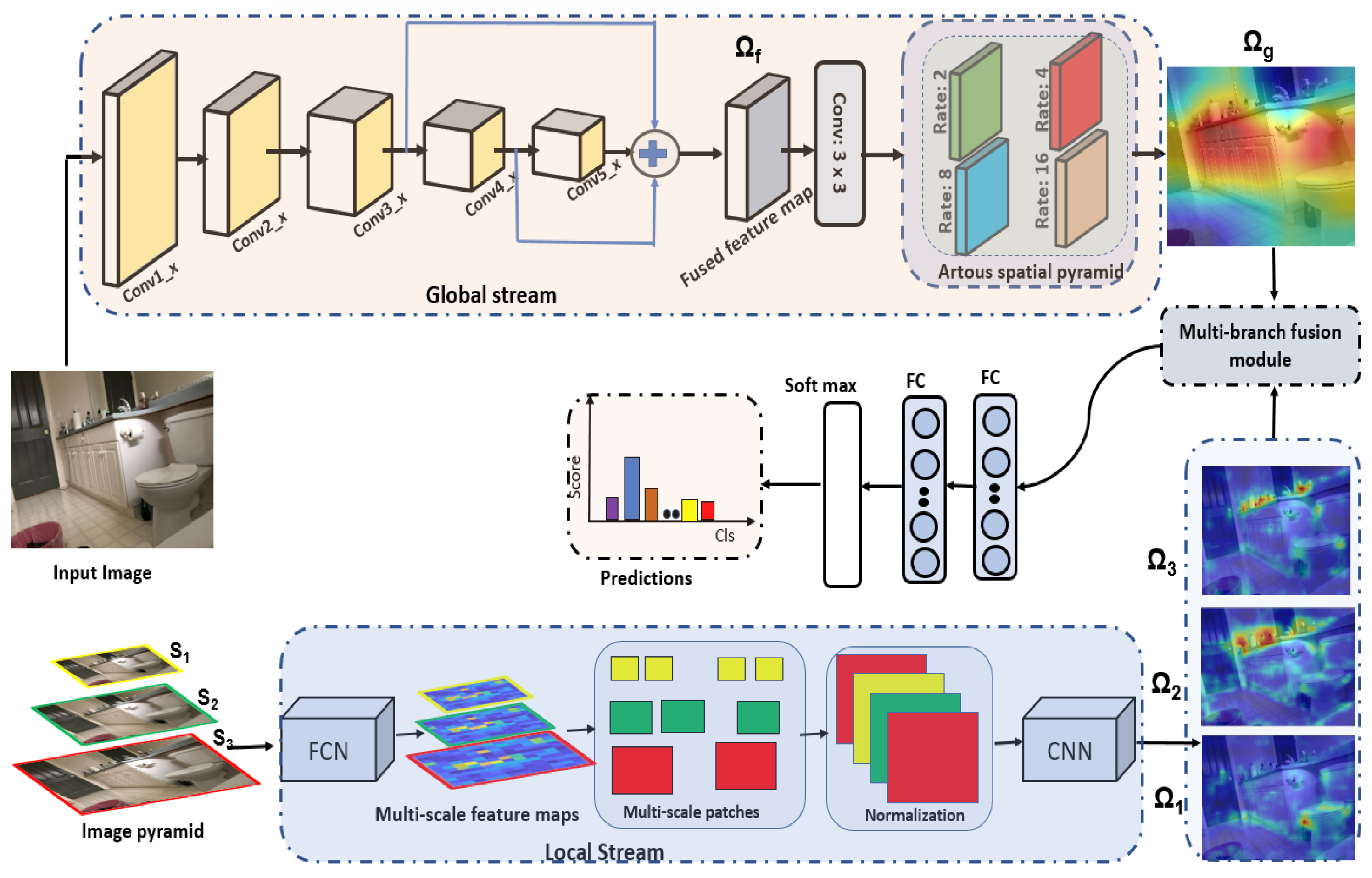
In this section, we discuss the architecture and detailed pipeline of the proposed framework for indoor scene recognition. The overall pipeline of proposed framework is illustrated in Figure 1. Generally, the framework consists of two streams, namely, a global stream and a local stream. Both these streams consists of deep learning models responsible for extracting local and global information from the scene to aid the scene recognition task. We provide details of each stream below.
3.1. Global Stream
The global stream is a critical component of the overall architecture designed to understand the global context and semantic information present in the input image. It aims to capture high-level features and relationships between different regions, objects, or structures in the scene. To achieve this, the global stream utilizes a deep learning model as its backbone, which forms the core framework for processing the image data. The backbone model consists of several layers, including convolutional layers responsible for feature extraction and down-sampling pooling layers. These layers automatically extract hierarchical features and learn complex representations from the input image. Notably, the shallow layers of the model learns low-level features, including, edges, texture, corner, etc, while the high-order layers extract semantic and global information of the scene.
The global stream allows for the utilization of any deep learning model as its backbone, including ResNet [50], DenseNet [51], VGG-16 [52], etc. However, in this particular work, we use VGG-16 as the backbone model. VGG-16 is selected for its exceptional performance and success in diverse computer vision tasks, especially scene recognition and object detection. The network’s deep architecture enables it to effectively capture complex patterns and contextual information, making it highly suitable for understanding complex scenes with varying scales and detailed objects.
While VGG-16 has achieved remarkable success in numerous object detection and scene recognition tasks, it faces challenges when applied to indoor scene recognition. This is because indoor scenes are associated with unique challenges, including the complexity of indoor scenes, diverse objects with different sizes, scales and colors, complex textures, and varying lighting conditions. Furthermore, indoor scenes demand fine-grained recognition capabilities to distinguish subtle differences between similar categories. For example, it is challenging for the model to distinguish the difference between a living room and a drawing room or bedroom. Because of this, the original VGG-16 model encounters setbacks when applied to indoor scene recognition tasks.
To address the aforementioned challenges, it is desirable to modify the original VGG-16 architecture to enable it to extract (1) multi-scale features and (2) global contextual information.

Figure 1.
Detailed architecture of proposed framework for indoor scene classification.
Figure 1.
Detailed architecture of proposed framework for indoor scene classification.
3.1.1. Extracting Multi-Scale Features
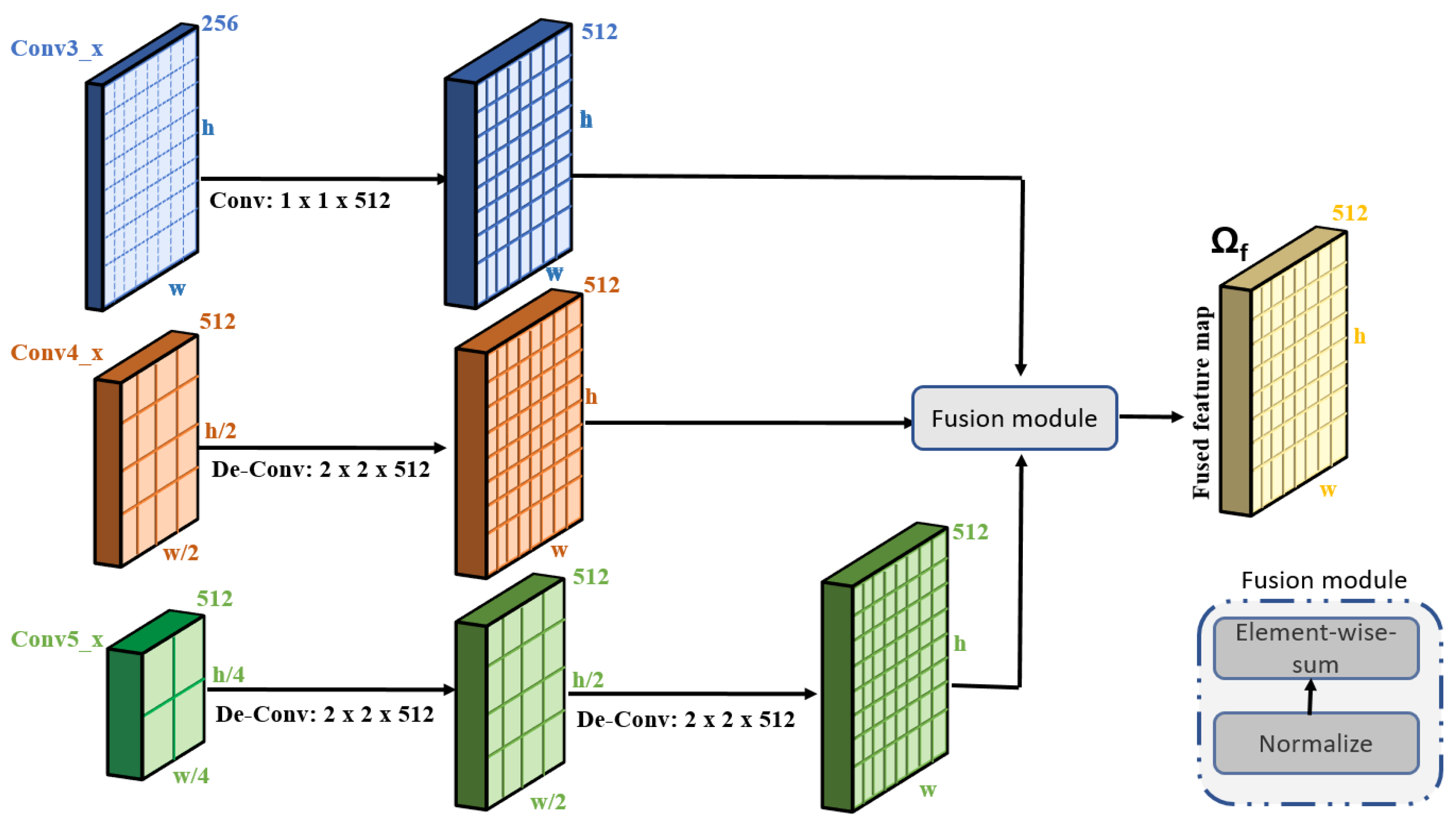
Multi-scale features refer to representations of the input image at multiple resolutions or levels of detail. These features encompass information about both fine details and broader spatial contexts within the scene. In indoor environments, where scenes often comprise various objects and elements of different scales and sizes, the utilization of multi-scale features becomes particularly significant. To extract multi-scale features, we utilize the feature maps from multiple layers of the network, each representing different scales of information. For example, feature maps from early layers, such as conv2_x capture fine details and local textures due to their smaller receptive fields. These feature maps are well suited for extracting fine-grained information about small objects within the scene. Conversely, feature maps from deeper layers, such as conv5_x, encompass larger receptive fields and encode higher-level semantic information about the scene, including spatial relationships between objects and overall scene context [53,54]. By combining feature maps from multiple layers of VGG-16, we obtained a multi-scale representation of the input image. This multi-scale representation preserves both fine-grained details and global spatial information, facilitating more comprehensive scene understanding and improved performance in tasks such as indoor scene classification.
To capture multi-scale features, we make modifications to the original VGG-16 architecture. We utilize the three convolutional layers of the VGG-16, namely, conv3_x, conv4_x, and conv5_x. The overall mechanism of extracting multi-scale features is illustrated in Figure 2. As is obvious from Figure 2, the sizes of the feature maps of these three layers are not same. The size of the feature map of the conv5_x layer is half the size of that of conv4_x. Similarly, the feature map of conv4_x is half the size of the feature map of conv3_x. It is to be noted that convolutional layer conv3_x contains information about the small objects, conv4_x contains information about the medium objects, while conv5_x contains information about the large objects. To combine the feature maps of these three layers, it is important to re-size the feature maps of these layers to make them suitable for the fusion process. In order to do this, we employ one deconvolution operation (of size 2 × 2) on to upscale the size of the feature map equal to the size of . Similarly, we employ two deconvolution operations on (each of size 2 × 2) to upscale the size of the feature map equal to the size of . After aligning the feature maps to the same size, we first normalize the feature maps and employ element-wise addition to fuse the feature maps from the three layers. Let be the final fused feature map. The feature map now contains multi-scale information, providing valuable assistance in boosting the classification accuracy. The detailed architecture of the global stream model is provided in Table 1.
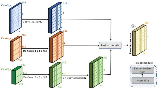
Figure 2.
Fusion mechanism for extracting multi-scale features from different layers of VGG-16.

Table 1.
Detailed architecture of global stream model.
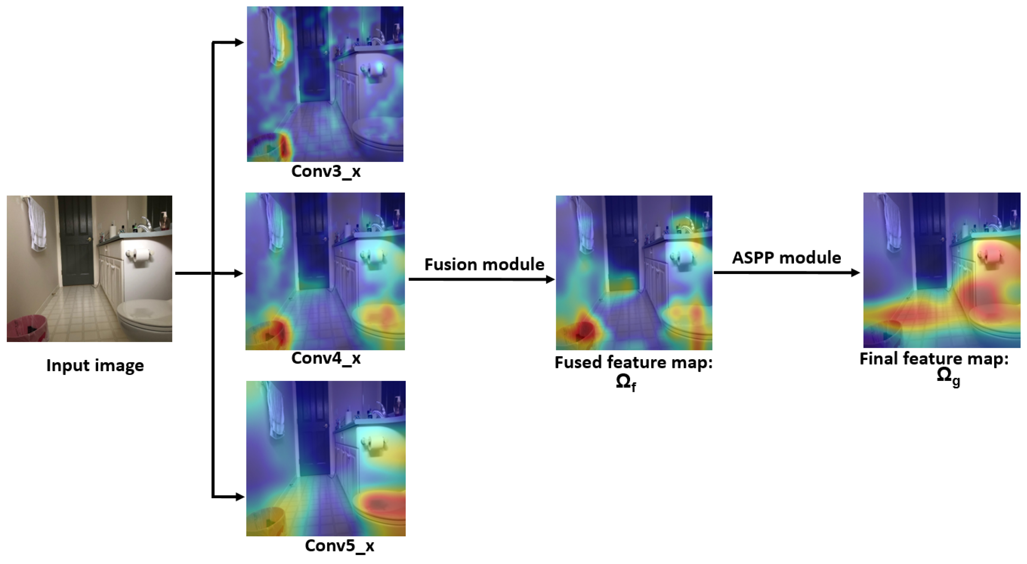
Figure 3 illustrates a visualization of the global stream. The input image is applied to the global stream. The global stream exploits the feature maps of the conv3_x, conv4_x, and conv5_x convolutional layers. From Figure 3, it is evident that the conv3_x layer captures details of the small objects, while conv5_x captures details of the large objects in the image. These features are then combined by fusion modules to generate a fusion feature map . To further enrich this representation with global contextual information, the feature map undergoes further processing via the ASPP module, thereby enhancing its global context. When comparing the fused feature map with the final feature map , it becomes evident that the ASPP modules enhance the global context by exhibiting maximum activation (depicted in reddish color) over crucial regions that aid in the classification task.

Figure 3.
Visualization of feature maps from conv3_x, conv4_x, and conv5_x. The feature maps are then combined with a fusion module to generate , which is then passed through an ASPP module to generate the final feature map .
3.1.2. Extracting Local Contextual Information
While the fused feature map contains multi-scale information, it may lack rich contextual information. Therefore, we employ an atrous spatial pyramid pooling (ASPP) module [55] to extract rich contextual information from the input image. The ASPP module captures contextual information at different spatial scales and enables the network to analyze the entire image and incorporate context from various scales. For this purpose, we provide as an input to the atrous spatial pyramid pooling module, which employs atrous convolutions at multiple dilation rates (2, 4, 8, 16) to gather both local and global context from various spatial scales. Let be the feature map obtained after employing the ASPP module. The now contains multi-scale information as well as fine-grained local details alongside broader contextual information.
3.2. Local Stream
Global contextual information alone is not enough to achieve high accuracy for the indoor scene classification task. It is important to obtain fine-grained local information as well to boost the performance. By incorporating fine-grained local information, the model gains the ability to obtain detailed information from nearby areas, allowing the model to recognize complex scenes. The local fine-grained information provides support to the model to discriminate different scenes sharing a similar global layout but different localized objects. To achieve this objective, we employ a fully convolutional-based object detection model. This specialized model is capable of detecting various objects within the scene. The features extracted from these localized objects are then merged with the global stream model, creating discriminative feature maps. By combining the information from both local and global sources, we enhance the model’s ability to discern and distinguish between different objects and scenes effectively.
To obtain fine-grained local information of the objects, it is imperative to know the location of various objects in the scene. In order to achieve this, we employ two different networks in the local stream. Generally, the local stream consists of two deep learning networks. The first network is called the objectness network, which generates a large number of scale-aware object proposals and predicts the objectness score for different proposals. The second module is the object classification network, which classifies the object proposals into specific categories.
The objectness network is a fully convolutional network designed to predict the objectness score for different regions of an input image. Generally, the objectness network is a binary classifier, which classifies each proposal into two categories—foreground objects or background. In this context, the network only classifies proposals obtained from the input image as containing an object or not. In other words, the objectness network provides the likelihood of regions containing objects. The input of the objectness network is an arbitrary size image and the output is the objectness map. Each pixel in the objectness map represents the presence of the object in the scene. The darker the pixel, the higher is the probability of the foreground objects, while the blueish pixels represent the background. We then employ blob analysis on the objectness map to obtain multi-scale region proposals.
To train the objectness network, we adopt patch-level training instead of a whole image. In this strategy, we divide the image into multiple overlapped patches. We then annotate each patch as positive (contain foreground objects) or negative patches (background). We use the following objective function to optimize the loss and formulated as Equation (1):
where N represents the total number of patches, and and represent the ground truth and predicted class of patch i, respectively.
After generating the object proposals, the next step is to classify each proposal into a specific class. For this purpose, we employ another deep learning model which has a similar structure to the objectness network. However, unlike the proposal generation network that predicts binary labels, the classification model assigns each proposal to specific pre-defined categories. For training, we use the same patch-wise training strategy as we did for training the proposal generation network. The key distinction is that we now assign class labels to each patch instead of utilizing binary labels to generate objectness maps. The detailed architecture of the local stream model is illustrated in Table 2. It is to be noted that the local stream model follows the pipeline of VGG-16. Initially, we train the VGG-16 on the dataset and then, during the inference stage, we utilize the four convolutional blocks of the network.

Table 2.
Detailed architecture of local stream model.
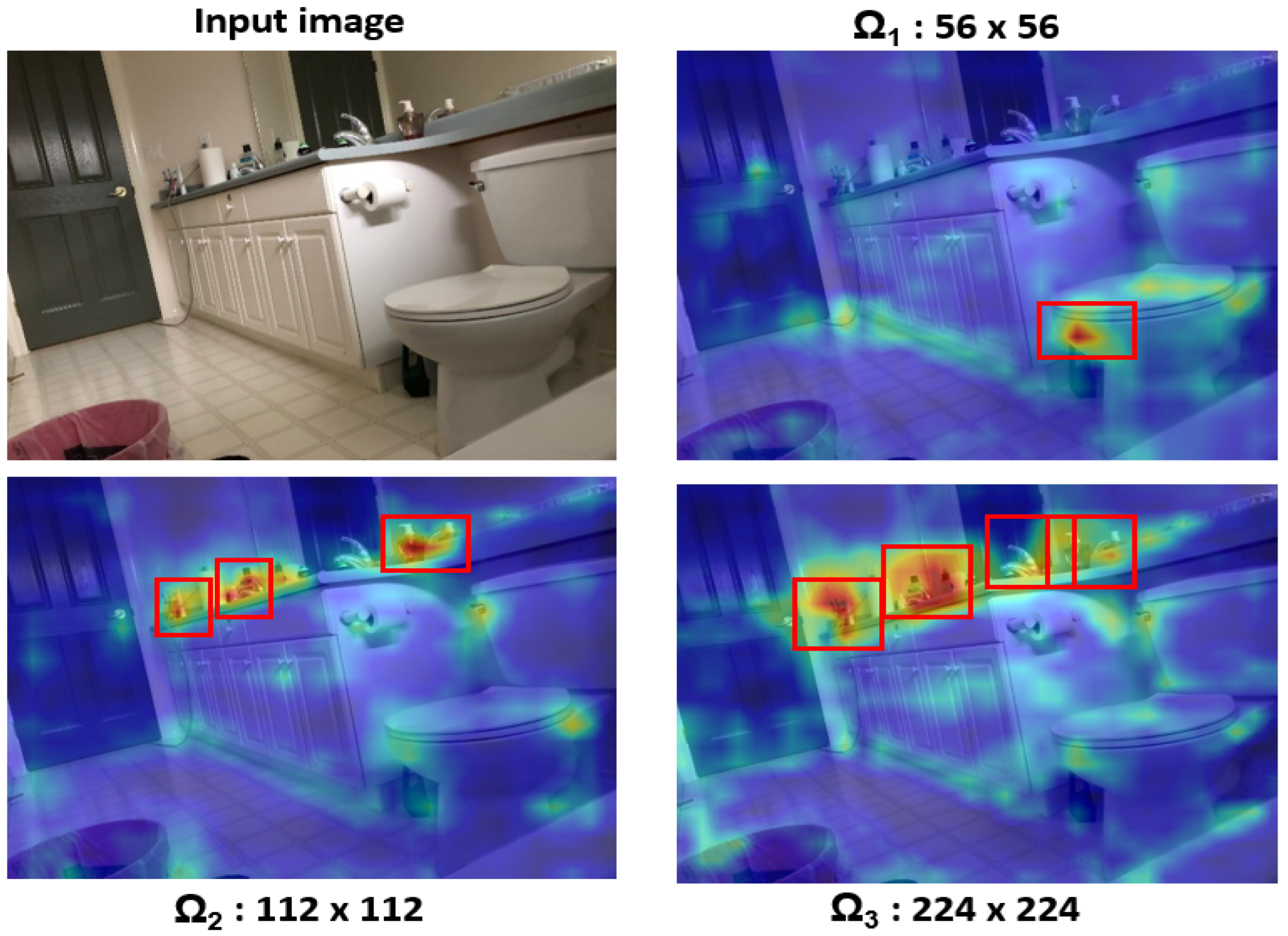
In our experimentation, we implemented an image pyramid consisting of three levels, . This approach involved resizing the input image into three distinct sizes, each subsequently fed into the network. Consequently, the network produced three separate objectness maps, each corresponding to one of the resized images. Specifically, our experiments utilized an image pyramid with sizes of 56 × 56, 112 × 112, and 224 × 224. Let correspond to scale 56 × 56, to 112 × 112, and correspond to scale 224 × 224. This will generate three scales of the input image by resizing it accordingly. Subsequently, each resized image was provided to the local stream, resulting in the generation of corresponding heatmaps. Let , , and be the corresponding heatmaps.
Figure 4 depicts the heatmaps obtained from the different scales. Initially, the input image was resized to a scale of 56 × 56 before being inputted into the local stream. The resulting feature map was then resized to match the size of the input image. Similarly, heatmaps were generated for scales of 112 × 112 and 224 × 224. From the Figure 4, it is evident that the local stream model focuses on localized regions, as indicated by bounding boxes highlighted in red. It is worth mentioning that while the global stream model prioritizes capturing information about large objects and global context, the local stream model aims to capture details of smaller objects. For instance, in Figure 4, the local stream effectively detects various local objects, such as tap water, bottles, and toothbrushes, etc. This localized information is crucial for scene recognition, as these objects are typically found in settings like bathrooms rather than in other areas like living rooms.

Figure 4.
Original input image and corresponding heatmaps at scales of 56 × 56, 112 × 112, and 224 × 224, showcasing the local stream’s focus on capturing details of local objects essential for scene recognition.
The multi-branch fusion module combines feature maps from both the local (, , ) and global streams (). Initially, it ensures that both feature maps are resized to match the same dimensions of the input image. To do this, the feature maps from the local stream (, , ) are re-sized to 224 × 224. Similarly, the feature map from the global stream () is also re-sized to 224 × 224. Subsequently, element-wise addition is performed on these feature maps to produce a final fused map. This final fused map is then fed into the fully connected layers, followed by a softmax classifier, to yield the final score for the input image.
We implement the proposed framework using the PyTorch library [56]. We utilize the Adam optimizer [57] and apply the cross-entropy loss function to all models. Both the local and global stream models undergo training for 60 epochs with a batch size of 64, and the initial learning rate is set to 0.0001. The learning rate undergoes consistent updates, being divided by 10 after every 10 epochs.
4. Experiment Results
In this section, we discuss the experimental results for indoor scene classification, and provide a comprehensive analysis of the outcomes achieved through the evaluation and comparisons with state-of-the-art methods. In this section, we also provide details of the range of performance metrics used to evaluate the performance of the proposed framework and also details of the dataset curated for indoor scene classification.
4.1. Dataset
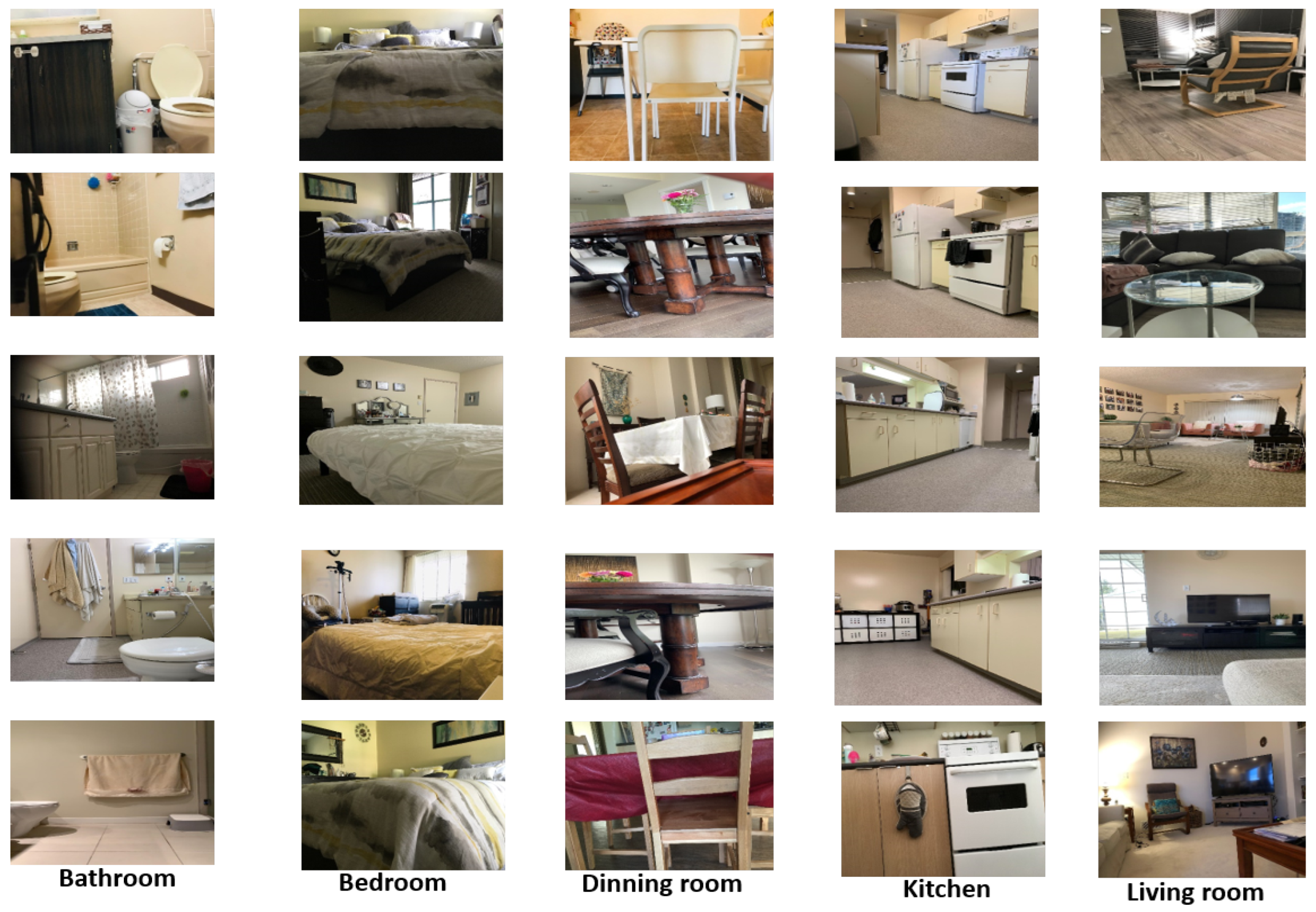
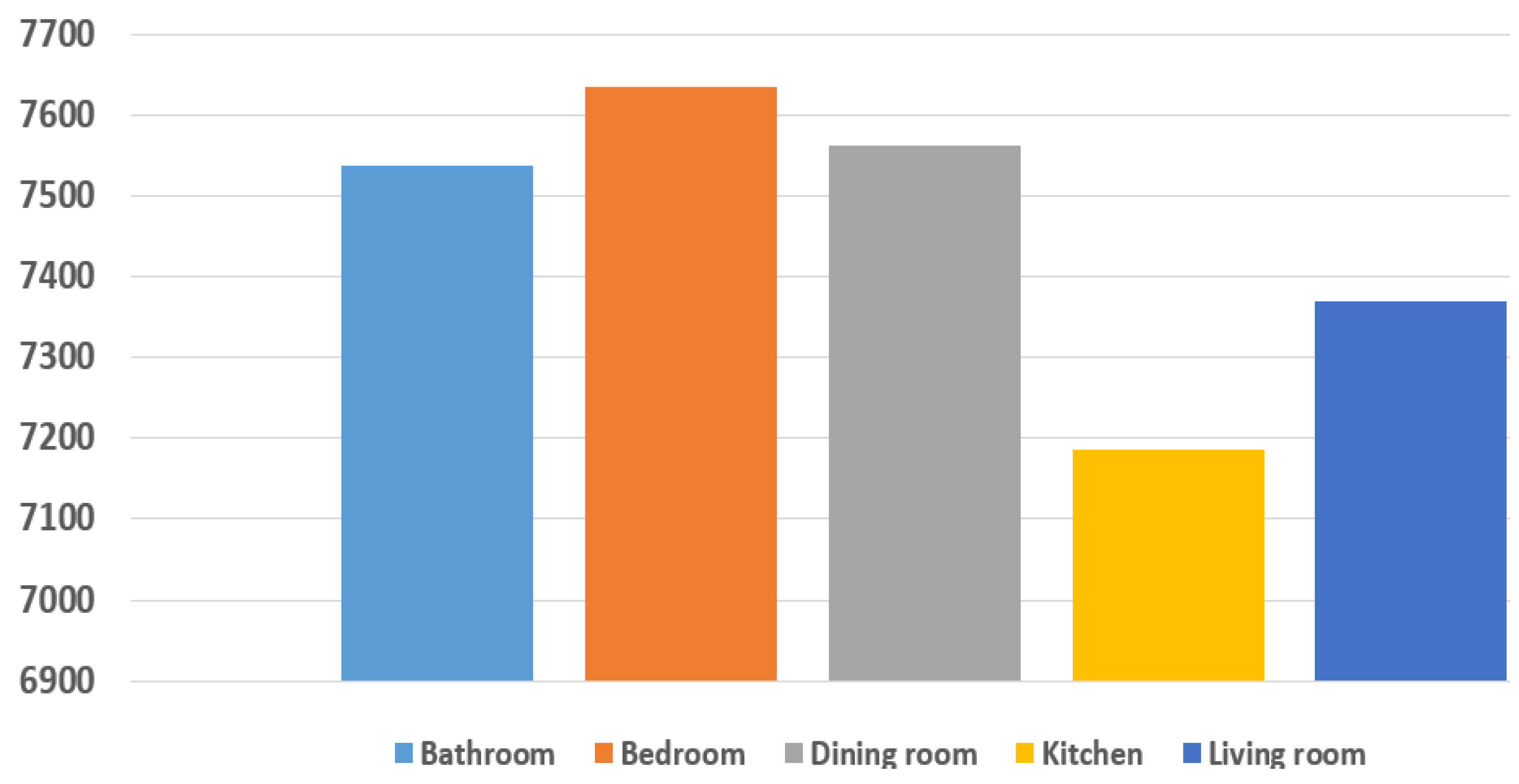
In this study, we employ the SRIN dataset as the foundation for our indoor scene classification task. The SRIN dataset, originally compiled by Othman et al. [58], is derived from indoor scenes within various residences in Vancouver city. This dataset comprises five distinct classes, including bathrooms, kitchens, dining rooms, living rooms, and bedrooms, with each class containing a set of 37,288 images. These images capture scenes from diverse perspectives, varying angles, and varying distances from the camera, all from a robotic viewpoint rather than a human’s perspective. The average resolution of the images in our dataset is 1600 × 1200 pixels, captured from a camera on a Nao humanoid robot of height 0.6 m with an approximate field of view ranging from 30 to 45 degrees. We found this resolution and field of view to be sufficient for capturing detailed information in indoor scenes. The dataset is challenging due to several factors, including the diversity of scenes captured, variations in lighting conditions, complex object interactions, and the presence of ambiguities in certain images. The samples from each class are illustrated in Figure 5, while Figure 6 shows the samples per class.

Figure 5.
Samples of different categories from SRIN dataset. The first column represents the samples of the Bathroom class. The second column represents the samples from the Bedroom class, the third column represents samples from the Dining room class, and the fourth and fifth columns represent samples from the Kitchen and Living room classes, respectively.

Figure 6.
Distribution of samples per class.
To address the limited number of samples per class and prevent overfitting, we utilize augmentation techniques to expand the training dataset. For this purpose, we apply various transformations, such as rotations, translations, flips, and adding noise, to the existing dataset, effectively creating new variations of the data. We believe that the augmentation technique not only increases the size of the dataset but also introduces diversity, which may help the model to learn more robust and generalizable features. For both training and testing, we adhere to the same approach as employed by [58], allocating 29,832 samples for training and reserving the remainder for testing.
4.2. Evaluation Metrics
In the context of indoor scene classification, the careful choice of evaluation metrics plays a pivotal role in accurately gauging a model’s performance. Commonly used evaluation metrics to assess the performance of models include precision, recall, the F1-score, and confusion matrices.
Precision measures the model’s capacity to precisely identify indoor scenes, with a focus on minimizing incorrect identifications and formulated as . Recall assesses how well the model can identify all indoor scenes correctly, with an emphasis on minimizing instances of false negatives and formulated as . Confusion matrices, on the other hand, measure the overall performance of the framework, offering valuable insights into the model’s classification performance.
To evaluate the effectiveness of the proposed framework, we report the performance in terms of a confusion matrix, as illustrated in Figure 7. Figure 7 represents the performance of the proposed framework in predicting the five different classes (Bathroom, Bedroom, Dining room, Kitchen, and Living room). From the Figure 7, it is observed that the proposed framework achieves 100% accuracy in predicting the Bathroom, Bedroom, and Dining room classes. However, we observe that the proposed framework faces challenges in precisely predicting the Kitchen class; it is clear from the confusion matrix that the framework misclassifies 8.3% of instances of the Kitchen class as the Bathroom class. This is because both the classes share similar features or characteristics. A similar case was observed in the Living room class, where the model misclassifies 6.2% of instances of the Living room class as Bedroom.
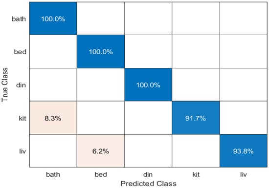
Figure 7.
Performance of the proposed framework in terms of a confusion matrix. Each row in the matrix represents the true class, while each column represents the predicted class. The values in the matrix indicate the percentage of instances that were correctly or incorrectly classified.
The proposed framework demonstrates exceptional performance in scene classification, as is evident from the precision, recall, and F1-score values presented in Table 3. From Table 3, it is obvious that the proposed framework achieved 100% precision in all the classes, while the framework achieved a 100% recall rate and F1-score in the Bathroom, Bedroom, and Dining room classes. The framework also achieved a more than 90% recall rate and F1-score in the complicated classes, which include the Kitchen and Living room classes. Such high performance across the board reflects the robustness and accuracy of the framework in categorizing scenes.

Table 3.
Performance of proposed framework in terms of precision, recall, and F1-score.
This impressive performance can be attributed to the dual-branch architecture of the proposed framework. The first branch is responsible for extracting global features from the input data. These global features provide a broad understanding of the scene, allowing the model to grasp high-level information. Simultaneously, the second branch focuses on extracting multi-scale local discriminating features, which are crucial for scene classification. These local features enable the model to capture complex details and patterns within the scenes.
We compare the performance of various deep learning models, including, AlexNet [59], VGG-16 [52], ResNet-50 [50], ResNet-152 [50], EfficientNet [60], DenseNet-121 [51], ShuffleNet [61], MobileNet [62] in Table 4. Table 4 presents a comprehensive performance comparison of deep learning models applied to the task of scene characterization across various indoor scenes. Each method’s performance is evaluated based on precision (P), recall (R), and the F1-score, providing a detailed insight into their ability to accurately identify and classify scenes. From Table 4, it is obvious that moderate performance is demonstrated across all scenes. The prime reason behind the moderate performance of AlexNet is the simplicity of its architecture. AlexNet has fewer layers and is not capable of extracting deep discriminating features, especially in complex patterns and scenes like kitchens and living rooms. Furthermore, AlexNet may struggle with the scale variation and hierarchical features that are vital for scene recognition. Similarly, VGG-16 exhibits relatively lower performance in scene characterization compared to the other methods. One of the major reasons for its lower performance is that VGG-16 has a significantly larger number of layers compared to models like EfficientNet and MobileNet, which makes it more prone to overfitting when the training data are limited. The overfitting problem reduces the models ability to generalize to unseen scenes. On the other hand, DenseNet-121 consistently performs well across all scenes with F1-scores ranging from 85.1% to 91.5%. This is because the dense connectivity allows the model to capture a wide range of features, effectively enabling the model to be adept at recognizing different scenes. EfficientNet achieves good performance with F1-scores ranging from 90.4% to 94.5% across all the scenes. This is due to the efficient architecture of the model (a balance between the model’s size and performance), which captures relevant features efficiently, enabling the model to recognize complex scenes accurately. In contrast to the reference methods, the proposed approach consistently outperforms them in all scene categories. This superior performance can be attributed to the dual-branch architecture of the proposed framework, which is a key innovation that adeptly fuses global and local information. The global branch enables the framework to capture the overall context and semantic details within the input image, whereas the local branch plays a pivotal role in enhancing the model’s capacity to distinguish between scenes that share similar global layouts but distinct localized objects.

Table 4.
Performance comparison of different methods in characterizing different scenes. P represents the precision, R represents recall and F1 shows the F1-score.
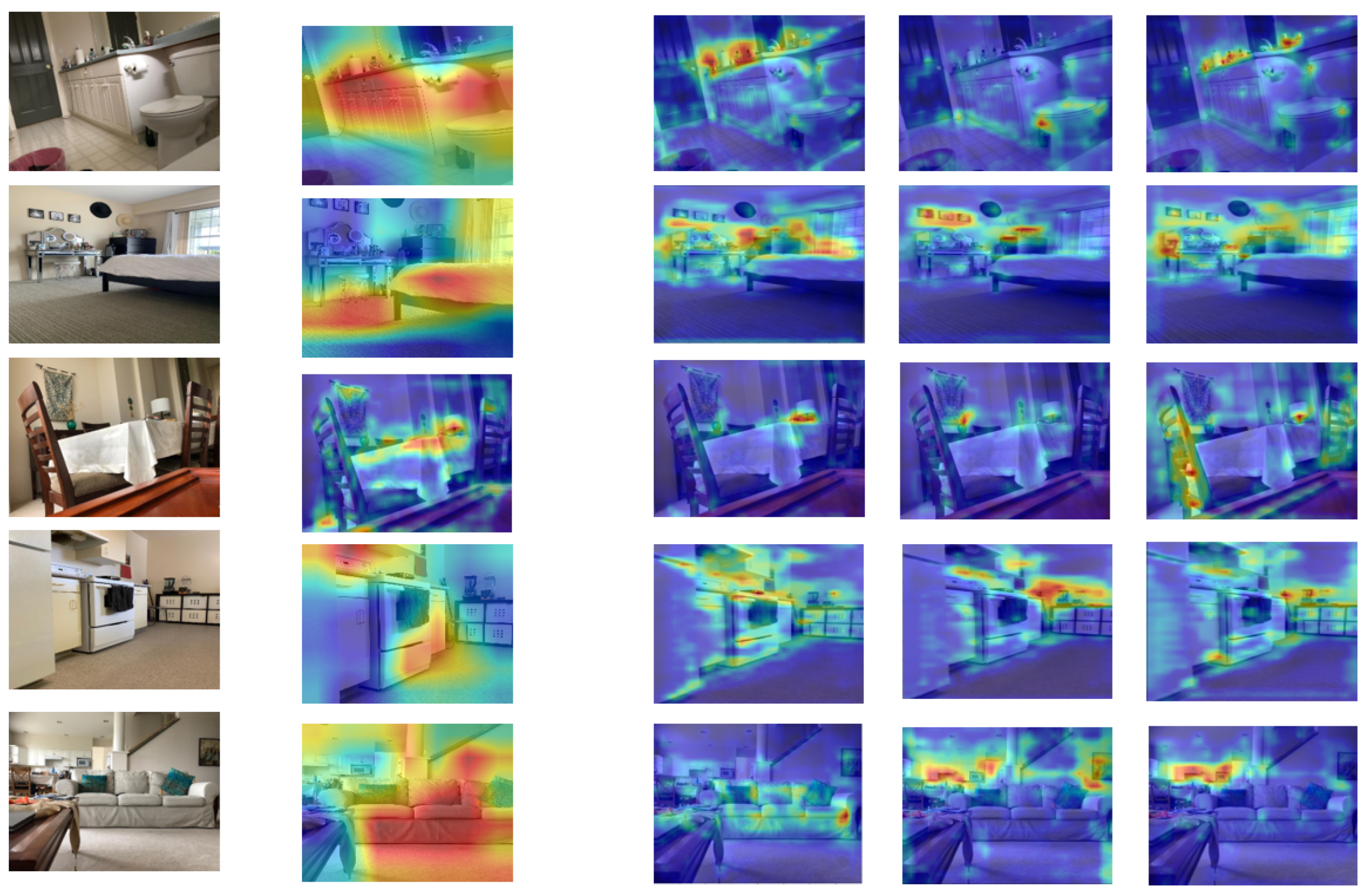
In Figure 8, we present a visualization of the feature maps originating from both the local and global streams within the proposed framework. This allows us to visualize the inner working of different streams of the framework and to understand how the network triggers activations in different layers for specific features, textures, and objects.
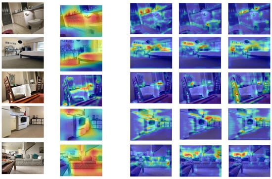
Figure 8.
Visualization of feature maps obtained from both the local and global streams of the proposed framework, showcasing their respective contributions in capturing local details and global context within the input image. The first column shows the random sample frames, the second column shows the output of the feature map of the global stream, while the 3rd, 4th, and 5th columns represent the feature maps of the local stream.
From Figure 8, it is obvious that the feature maps obtained from the global streams have activations spread over the whole image. These activations provide valuable insights into what the network deems important when making high-level decisions about the input image. This is because the global stream utilizes the feature map of the last convolutional layer that captures the global context which represents the whole input image. We observe that the feature map obtained from the global stream emphasizes the presence of large objects, background structures, and spatial arrangements that are critical for recognizing the global context of the scene. The feature map obtained from the local stream captures local details and activations that are concentrated in specific, localized regions of the image rather than being spread across the entire image. This implies that the local stream pays attention and is responsive to particular areas within the input. For example, if the input image represents a kitchen scene, the feature map may highlight details such as the texture of the countertop, the appearance of the kitchen utensils, or the arrangement of the items on a shelf. The activations in such feature maps are closely tied to these local elements, emphasizing the network’s capability to recognize and emphasize fine-grained information that is crucial for understanding the localized characteristics of the scene.
5. Ablation Study
In this section, we describe an ablation study to analyze the influence of both local and global streams on the effectiveness of the proposed framework. Additionally, we aim to understand the impact of various factors, such as different backbone networks, the integration of multi-scale fusion, and the incorporation of ASPP modules, on the overall performance of the framework. Through this analysis, we seek to gain deeper insights into the contributions of these elements towards achieving optimal performance in our framework. For the ablation study, we use nine different configurations. The ablation study is presented in Table 5. We provide the details of each configuration as follows:

Table 5.
Ablation study to evaluate the effect of local and global streams along with backbone network on the performance.
- Configuration C1 utilizes the VGG-16 backbone network in the global stream without incorporating multi-scale features or ASPP. Furthermore, this configuration does not include a local stream.
- C2 builds upon C1 by introducing multi-scale processing in the global stream. This configuration does not incorporate an ASPP module and local stream.
- C3 further enhances the global stream by incorporating ASPP along with multi-scale processing; however, a local stream is missing.
- Configuration C4 does not include a global stream; however, it employs a local stream with VGG-16 as the backbone of the FCN and CNN networks.
- Configuration C5 integrates both global and local streams, leveraging the VGG-16 backbone network in the global stream along with multi-scale fusion and ASPP modules. In the local stream, it utilizes the ResNet architecture for both the FCN and CNN networks.
- Configuration C6 adopts ResNet as the backbone network for the global stream, incorporating multi-scale fusion and ASPP modules. Similar to C5, it utilizes ResNet in the local stream as well.
- Configuration C7 utilizes DenseNet in the global stream along with multi-scale fusion and ASPP modules. In the local stream, it employs ResNet.
- Configuration C8 utilizes EfficientNet as the backbone network in the global stream along with multi-scale fusion and ASPP modules and DenseNet in the local stream.
- Configuration C8 utilizes DenseNet as the backbone network in the global stream along with multi-scale fusion and ASPP modules and DenseNet in the local stream.
The performance of these different configurations is measured using the average precision, recall, and F1-score across all the classes of the dataset. Comparing the performance of C1, C2, C3, C4, and C5 allows us to understand the effect of multi-scale and ASPP modules, as well as the importance of local and global streams. From Table 5, it is evident that configuration C1 performs relatively poorly. This can be attributed to the fact that C1 solely relies on the VGG-16 backbone network. The issue with this configuration is that the network utilizes the feature map of the last convolutional layer for classification. The receptive field of the last convolutional layer is large, which may capture details of large objects but may miss important information about smaller objects. In contrast to this method, configuration C2 utilizes multi-scale features, as discussed in Section 3.1.1. However, performance further improves with the incorporation of the ASPP module in configuration C3. Additionally, from Table 5, we also recognize the importance of local and global stream modules. The performance of C4 is lower compared to C5, which incorporates the global stream with multi-scale and ASPP modules, along with the local stream.
Furthermore, the performance of configurations C6, C7, C8, and C9 provides insights into the effect of different backbone architectures in both local and global streams. Configurations C6, C7, C8, and C9 each utilize distinct backbone networks, including ResNet, DenseNet, and EfficientNet, in various combinations across the global and local streams. From Table 5, it is evident that despite the differences in backbone architectures, the performance improvements observed among these configurations may not be notably significant to report. This may be because indoor scenes often exhibit relatively consistent visual characteristics compared to more diverse outdoor environments. As a result, the architectural differences of backbone networks may not significantly impact performance when distinguishing between indoor scenes.
6. Time Complexity
In this section, we evaluate the performance of different models along with the proposed method in terms of computational complexity during the inference time. Time complexity is an important measure to understand the computational requirement of the model and its applicability in real time or near to real time. The time complexity of different models is provided in Table 6. From Table 6, it is evident that AlexNet take less inference time compared to the other models. This is because AlexNet has a very simple architecture with a limited number of layers. On the other hand, ResNet-50 and DenseNet-121, despite dense connections and a complex architecture, achieve good inference time. The proposed method, however, lags behind the reference models due to the complex architecture of the framework. Despite a high reference time, the model achieves good results in terms of average precision, recall, and F1-score rates. This analysis shows that our proposed method strikes an optimal balance between execution time and accuracy, despite its higher computational demands compared to the reference models.

Table 6.
Time complexity comparisons of different models during the inference time (in seconds). Performance is measured in terms of average precision (Avg P), average recall (Avg R), and average F1-score (Avg F1).
7. Conclusions
In this work, we present a dual-stream framework for indoor scene classification, which is a crucial task for enabling effective navigation and interaction of social robots within diverse indoor environments. The framework addresses the problems of inter-class similarity and intra-class variance by proposing a global–local stream architecture. The global stream of the framework captures high-level features and relationships across different regions and objects, while the local stream employs fully convolutional networks to extract detailed local information. Our experiments on a challenging dataset have showcased the effectiveness of this dual-stream framework, which outperforms existing methods across various indoor scenes.
The proposed dual deep learning framework can be integrated with other vehicle technologies, such as LiDAR and radar, to enhance situational awareness and improve decision-making in autonomous vehicles. For example, integrating our proposed framework with LiDAR can enable more accurate scene understanding by incorporating detailed 3D information alongside visual data. Moreover, radar can complement our framework by providing additional information about the velocity and trajectory of objects, enhancing the vehicle’s ability to predict and respond to dynamic scenarios.
The research findings of the proposed framework may inspire future innovations in autonomous vehicle solutions in enhancing scene understanding and navigation. By demonstrating the capability to accurately classify complex indoor scenes, our research paves the way for more intelligent and adaptable autonomous vehicles capable of navigating diverse environments with greater precision and safety. Furthermore, in future work, we will optimize the proposed framework to make it suitable for real-time applications without compromising its performance.
Author Contributions
Conceptualization, S.D.K. and K.M.O.; methodology, S.D.K.; software, S.D.K.; validation, K.M.O.; formal analysis, S.D.K.; investigation, S.D.K.; resources, K.M.O.; data curation, K.M.O.; writing—original draft preparation, S.D.K.; writing—review and editing, K.M.O.; visualization, K.M.O.; supervision, S.D.K.; project administration, S.D.K.; funding acquisition, K.M.O. All authors have read and agreed to the published version of the manuscript.
Funding
This research received no external funding.
Data Availability Statement
The data used in the research is publicly available.
Conflicts of Interest
The authors declare no conflicts of interest.
References
- Choe, S.; Seong, H.; Kim, E. Indoor place category recognition for a cleaning robot by fusing a probabilistic approach and deep learning. IEEE Trans. Cybern. 2021, 52, 7265–7276. [Google Scholar] [CrossRef]
- Fragapane, G.; De Koster, R.; Sgarbossa, F.; Strandhagen, J.O. Planning and control of autonomous mobile robots for intralogistics: Literature review and research agenda. Eur. J. Oper. Res. 2021, 294, 405–426. [Google Scholar] [CrossRef]
- Ozkil, A.G.; Fan, Z.; Dawids, S.; Aanes, H.; Kristensen, J.K.; Christensen, K.H. Service robots for hospitals: A case study of transportation tasks in a hospital. In Proceedings of the 2009 IEEE International Conference on Automation and Logistics, Shenyang, China, 5–7 August 2009; IEEE: Piscataway, NJ, USA, 2009; pp. 289–294. [Google Scholar]
- Kyrarini, M.; Lygerakis, F.; Rajavenkatanarayanan, A.; Sevastopoulos, C.; Nambiappan, H.R.; Chaitanya, K.K.; Babu, A.R.; Mathew, J.; Makedon, F. A survey of robots in healthcare. Technologies 2021, 9, 8. [Google Scholar] [CrossRef]
- Bertacchini, F.; Bilotta, E.; Pantano, P. Shopping with a robotic companion. Comput. Hum. Behav. 2017, 77, 382–395. [Google Scholar] [CrossRef]
- Garcia Ricardez, G.; Okada, S.; Koganti, N.; Yasuda, A.; Uriguen Eljuri, P.; Sano, T.; Yang, P.C.; El Hafi, L.; Yamamoto, M.; Takamatsu, J.; et al. Restock and straightening system for retail automation using compliant and mobile manipulation. Adv. Robot. 2020, 34, 235–249. [Google Scholar] [CrossRef]
- Javaid, M.; Haleem, A.; Singh, R.P.; Suman, R. Substantial capabilities of robotics in enhancing industry 4.0 implementation. Cogn. Robot. 2021, 1, 58–75. [Google Scholar] [CrossRef]
- Ma, S.; Jiang, H.; Han, M.; Xie, J.; Li, C. Research on automatic parking systems based on parking scene recognition. IEEE Access 2017, 5, 21901–21917. [Google Scholar] [CrossRef]
- Ni, J.; Shen, K.; Chen, Y.; Cao, W.; Yang, S.X. An improved deep network-based scene classification method for self-driving cars. IEEE Trans. Instrum. Meas. 2022, 71, 1–14. [Google Scholar] [CrossRef]
- Zhou, H.; Zhou, S. Scene categorization towards urban tunnel traffic by image quality assessment. J. Vis. Commun. Image Represent. 2019, 65, 102655. [Google Scholar] [CrossRef]
- Du, H.; Wang, W.; Wang, X.; Wang, Y. Autonomous landing scene recognition based on transfer learning for drones. J. Syst. Eng. Electron. 2023, 34, 28–35. [Google Scholar] [CrossRef]
- O’Mahony, N.; Campbell, S.; Krpalkova, L.; Riordan, D.; Walsh, J.; Murphy, A.; Ryan, C. Deep learning for visual navigation of unmanned ground vehicles: A review. In Proceedings of the 2018 29th Irish Signals and Systems Conference (ISSC), Belfast, UK, 21–22 June 2018; IEEE: Piscataway, NJ, USA, 2018; pp. 1–6. [Google Scholar]
- Ekici, M.; Seçkin, A.Ç.; Özek, A.; Karpuz, C. Warehouse drone: Indoor positioning and product counter with virtual fiducial markers. Drones 2022, 7, 3. [Google Scholar] [CrossRef]
- Asadi, K.; Suresh, A.K.; Ender, A.; Gotad, S.; Maniyar, S.; Anand, S.; Noghabaei, M.; Han, K.; Lobaton, E.; Wu, T. An integrated UGV-UAV system for construction site data collection. Autom. Constr. 2020, 112, 103068. [Google Scholar] [CrossRef]
- Wijayathunga, L.; Rassau, A.; Chai, D. Challenges and solutions for autonomous ground robot scene understanding and navigation in unstructured outdoor environments: A review. Appl. Sci. 2023, 13, 9877. [Google Scholar] [CrossRef]
- Tagarakis, A.C.; Kalaitzidis, D.; Filippou, E.; Benos, L.; Bochtis, D. 3d scenery construction of agricultural environments for robotics awareness. In Information and Communication Technologies for Agriculture—Theme III: Decision; Springer: Berlin/Heidelberg, Germany, 2022; pp. 125–142. [Google Scholar]
- Zhou, L.; Zhou, Z.; Hu, D. Scene classification using a multi-resolution bag-of-features model. Pattern Recognit. 2013, 46, 424–433. [Google Scholar] [CrossRef]
- Khan, N.Y.; McCane, B.; Wyvill, G. SIFT and SURF performance evaluation against various image deformations on benchmark dataset. In Proceedings of the 2011 International Conference on Digital Image Computing: Techniques and Applications, Noosa, QLD, Australia, 6–8 December 2011; IEEE: Piscataway, NJ, USA, 2011; pp. 501–506. [Google Scholar]
- Ayers, B.; Boutell, M. Home interior classification using SIFT keypoint histograms. In Proceedings of the 2007 IEEE Conference on Computer Vision and Pattern Recognition, Minneapolis, MN, USA, 17–22 June 2007; IEEE: Piscataway, NJ, USA, 2007; pp. 1–6. [Google Scholar]
- Bay, H.; Ess, A.; Tuytelaars, T.; Van Gool, L. Speeded-up robust features (SURF). Comput. Vis. Image Underst. 2008, 110, 346–359. [Google Scholar] [CrossRef]
- Giveki, D. Scale-space multi-view bag of words for scene categorization. Multimed. Tools Appl. 2021, 80, 1223–1245. [Google Scholar] [CrossRef]
- Li, T.; Mei, T.; Kweon, I.S.; Hua, X.S. Contextual bag-of-words for visual categorization. IEEE Trans. Circuits Syst. Video Technol. 2010, 21, 381–392. [Google Scholar] [CrossRef]
- Ergul, E.; Arica, N. Scene classification using spatial pyramid of latent topics. In Proceedings of the 2010 20th International Conference on Pattern Recognition, Istanbul, Turkey, 23–26 August 2010; IEEE: Piscataway, NJ, USA, 2010; pp. 3603–3606. [Google Scholar]
- Xie, L.; Lee, F.; Liu, L.; Yin, Z.; Yan, Y.; Wang, W.; Zhao, J.; Chen, Q. Improved spatial pyramid matching for scene recognition. Pattern Recognit. 2018, 82, 118–129. [Google Scholar] [CrossRef]
- Gu, G.; Li, F.; Zhao, Y.; Zhu, Z. Scene classification based on spatial pyramid representation by superpixel lattices and contextual visual features. Opt. Eng. 2012, 51, 017201. [Google Scholar] [CrossRef]
- Labinghisa, B.A.; Lee, D.M. Indoor localization system using deep learning based scene recognition. Multimed. Tools Appl. 2022, 81, 28405–28429. [Google Scholar] [CrossRef]
- Yee, P.S.; Lim, K.M.; Lee, C.P. DeepScene: Scene classification via convolutional neural network with spatial pyramid pooling. Expert Syst. Appl. 2022, 193, 116382. [Google Scholar] [CrossRef]
- Wozniak, P.; Afrisal, H.; Esparza, R.G.; Kwolek, B. Scene recognition for indoor localization of mobile robots using deep CNN. In Proceedings of the Computer Vision and Graphics: International Conference, ICCVG 2018, Warsaw, Poland, 17–19 September 2018; Proceedings. Springer: Berlin/Heidelberg, Germany, 2018; pp. 137–147. [Google Scholar]
- Soroush, R.; Baleghi, Y. NIR/RGB image fusion for scene classification using deep neural networks. Vis. Comput. 2022, 39, 2725–2739. [Google Scholar] [CrossRef]
- Heikel, E.; Espinosa-Leal, L. Indoor scene recognition via object detection and TF-IDF. J. Imaging 2022, 8, 209. [Google Scholar] [CrossRef] [PubMed]
- Biswas, M.; Buckchash, H.; Prasad, D.K. pNNCLR: Stochastic Pseudo Neighborhoods for Contrastive Learning based Unsupervised Representation Learning Problems. arXiv 2023, arXiv:2308.06983. [Google Scholar] [CrossRef]
- Swadzba, A.; Wachsmuth, S. Indoor scene classification using combined 3D and gist features. In Asian Conference on Computer Vision; Springer: Berlin/Heidelberg, Germany, 2010; pp. 201–215. [Google Scholar]
- Swadzba, A.; Wachsmuth, S. A detailed analysis of a new 3D spatial feature vector for indoor scene classification. Robot. Auton. Syst. 2014, 62, 646–662. [Google Scholar] [CrossRef]
- Li, X.; Guo, Y. Multi-level adaptive active learning for scene classification. In Proceedings of the Computer Vision–ECCV 2014: 13th European Conference, Zurich, Switzerland, 6–12 September 2014; Proceedings, Part VII 13. Springer: Berlin/Heidelberg, Germany, 2014; pp. 234–249. [Google Scholar]
- Yu, J.; Tao, D.; Rui, Y.; Cheng, J. Pairwise constraints based multiview features fusion for scene classification. Pattern Recognit. 2013, 46, 483–496. [Google Scholar] [CrossRef]
- Choi, W.; Chao, Y.W.; Pantofaru, C.; Savarese, S. Indoor scene understanding with geometric and semantic contexts. Int. J. Comput. Vis. 2015, 112, 204–220. [Google Scholar] [CrossRef]
- Han, Y.; Liu, G. Efficient learning of sample-specific discriminative features for scene classification. IEEE Signal Process. Lett. 2011, 18, 683–686. [Google Scholar] [CrossRef]
- Zuo, Z.; Wang, G.; Shuai, B.; Zhao, L.; Yang, Q.; Jiang, X. Learning discriminative and shareable features for scene classification. In Proceedings of the Computer Vision–ECCV 2014: 13th European Conference, Zurich, Switzerland, 6–12 September 2014; Proceedings, Part I 13. Springer: Berlin/Heidelberg, Germany, 2014; pp. 552–568. [Google Scholar]
- Espinace, P.; Kollar, T.; Soto, A.; Roy, N. Indoor scene recognition through object detection. In Proceedings of the 2010 IEEE International Conference on Robotics and Automation, Anchorage, AK, USA, 3–7 May 2010; IEEE: Piscataway, NJ, USA, 2010; pp. 1406–1413. [Google Scholar]
- Margolin, R.; Zelnik-Manor, L.; Tal, A. Otc: A novel local descriptor for scene classification. In Proceedings of the Computer Vision–ECCV 2014: 13th European Conference, Zurich, Switzerland, 6–12 September 2014; Proceedings, Part VII 13. Springer: Berlin/Heidelberg, Germany, 2014; pp. 377–391. [Google Scholar]
- Bai, S. Growing random forest on deep convolutional neural networks for scene categorization. Expert Syst. Appl. 2017, 71, 279–287. [Google Scholar] [CrossRef]
- Khan, S.H.; Hayat, M.; Porikli, F. Scene categorization with spectral features. In Proceedings of the IEEE International Conference on Computer Vision, Venice, Italy, 22–29 October 2017; pp. 5638–5648. [Google Scholar]
- Pereira, R.; Gonçalves, N.; Garrote, L.; Barros, T.; Lopes, A.; Nunes, U.J. Deep-learning based global and semantic feature fusion for indoor scene classification. In Proceedings of the 2020 IEEE International Conference on Autonomous Robot Systems and Competitions (ICARSC), Ponta Delgada, Portugal, 15–17 April 2020; IEEE: Piscataway, NJ, USA, 2020; pp. 67–73. [Google Scholar]
- Pereira, R.; Garrote, L.; Barros, T.; Lopes, A.; Nunes, U.J. A deep learning-based indoor scene classification approach enhanced with inter-object distance semantic features. In Proceedings of the 2021 IEEE/RSJ International Conference on Intelligent Robots and Systems (IROS), Prague, Czech Republic, 27 September–1 October 2021; IEEE: Piscataway, NJ, USA, 2021; pp. 32–38. [Google Scholar]
- Seong, H.; Hyun, J.; Kim, E. FOSNet: An end-to-end trainable deep neural network for scene recognition. IEEE Access 2020, 8, 82066–82077. [Google Scholar] [CrossRef]
- Hayat, M.; Khan, S.H.; Bennamoun, M.; An, S. A spatial layout and scale invariant feature representation for indoor scene classification. IEEE Trans. Image Process. 2016, 25, 4829–4841. [Google Scholar] [CrossRef]
- Guo, W.; Wu, R.; Chen, Y.; Zhu, X. Deep learning scene recognition method based on localization enhancement. Sensors 2018, 18, 3376. [Google Scholar] [CrossRef] [PubMed]
- Basu, A.; Petropoulakis, L.; Di Caterina, G.; Soraghan, J. Indoor home scene recognition using capsule neural networks. Procedia Comput. Sci. 2020, 167, 440–448. [Google Scholar] [CrossRef]
- Sun, N.; Zhu, X.; Liu, J.; Han, G. Indoor scene recognition based on deep learning and sparse representation. In Proceedings of the 2017 13th International Conference on Natural Computation, Fuzzy Systems and Knowledge Discovery (ICNC-FSKD), Guilin, China, 29–31 July 2017; IEEE: Piscataway, NJ, USA, 2017; pp. 844–849. [Google Scholar]
- He, K.; Zhang, X.; Ren, S.; Sun, J. Deep residual learning for image recognition. In Proceedings of the IEEE Conference on Computer Vision and Pattern Recognition, Las Vegas, NV, USA, 26 June–1 July 2016; pp. 770–778. [Google Scholar]
- Huang, G.; Liu, Z.; Van Der Maaten, L.; Weinberger, K.Q. Densely connected convolutional networks. In Proceedings of the IEEE Conference on Computer Vision and Pattern Recognition, Honolulu, HI, USA, 21–26 July 2017; pp. 4700–4708. [Google Scholar]
- Simonyan, K.; Zisserman, A. Very deep convolutional networks for large-scale image recognition. arXiv 2014, arXiv:1409.1556. [Google Scholar]
- Khan, S.D.; Basalamah, S. Multi-scale person localization with multi-stage deep sequential framework. Int. J. Comput. Intell. Syst. 2021, 14, 1217–1228. [Google Scholar] [CrossRef]
- Zhang, S.; He, G.; Chen, H.B.; Jing, N.; Wang, Q. Scale adaptive proposal network for object detection in remote sensing images. IEEE Geosci. Remote Sens. Lett. 2019, 16, 864–868. [Google Scholar] [CrossRef]
- Chen, L.C.; Papandreou, G.; Kokkinos, I.; Murphy, K.; Yuille, A.L. Deeplab: Semantic image segmentation with deep convolutional nets, atrous convolution, and fully connected crfs. IEEE Trans. Pattern Anal. Mach. Intell. 2017, 40, 834–848. [Google Scholar] [CrossRef] [PubMed]
- Paszke, A.; Gross, S.; Chintala, S.; Chanan, G.; Yang, E.; DeVito, Z.; Lin, Z.; Desmaison, A.; Antiga, L.; Lerer, A. Automatic Differentiation in Pytorch. 2017. Available online: https://openreview.net/pdf/25b8eee6c373d48b84e5e9c6e10e7cbbbce4ac73.pdf?ref=blog.premai.io (accessed on 23 March 2024).
- Kingma, D.P.; Ba, J. Adam: A method for stochastic optimization. arXiv 2014, arXiv:1412.6980. [Google Scholar]
- Othman, K.; Rad, A. SRIN: A new dataset for social robot indoor navigation. Glob. J. Eng. Sci. 2020, 4, 1–6. [Google Scholar] [CrossRef]
- Krizhevsky, A.; Sutskever, I.; Hinton, G.E. Imagenet classification with deep convolutional neural networks. In Proceedings of the Advances in Neural Information Processing Systems, Lake Tahoe, NV, USA, 3–6 December 2012; Volume 25. [Google Scholar]
- Tan, M.; Le, Q. Efficientnet: Rethinking model scaling for convolutional neural networks. In Proceedings of the International Conference on Machine Learning, PMLR, Long Beach, CA, USA, 9–15 June 2019; pp. 6105–6114. [Google Scholar]
- Zhang, X.; Zhou, X.; Lin, M.; Sun, J. Shufflenet: An extremely efficient convolutional neural network for mobile devices. In Proceedings of the IEEE Conference on Computer Vision and Pattern Recognition, Salt Lake City, UT, USA, 18–22 June 2018; pp. 6848–6856. [Google Scholar]
- Howard, A.G.; Zhu, M.; Chen, B.; Kalenichenko, D.; Wang, W.; Weyand, T.; Andreetto, M.; Adam, H. Mobilenets: Efficient convolutional neural networks for mobile vision applications. arXiv 2017, arXiv:1704.04861. [Google Scholar]
Disclaimer/Publisher’s Note: The statements, opinions and data contained in all publications are solely those of the individual author(s) and contributor(s) and not of MDPI and/or the editor(s). MDPI and/or the editor(s) disclaim responsibility for any injury to people or property resulting from any ideas, methods, instructions or products referred to in the content. |
© 2024 by the authors. Licensee MDPI, Basel, Switzerland. This article is an open access article distributed under the terms and conditions of the Creative Commons Attribution (CC BY) license (https://creativecommons.org/licenses/by/4.0/).

