Article

Program Equivalence in the Erlang Actor Model

by
Péter Bereczky
1,*,
Dániel Horpácsi
1,* and
Simon Thompson
1,2
1
Department of Programming Languages and Compilers, ELTE Eötvös Loránd University, 1117 Budapest, Hungary
2
School of Computing, University of Kent, Canterbury CT2 7NZ, UK
*
Authors to whom correspondence should be addressed.
Computers 2024, 13(11), 276; https://doi.org/10.3390/computers13110276
Submission received: 31 August 2024 / Revised: 4 October 2024 / Accepted: 16 October 2024 / Published: 23 October 2024
(This article belongs to the Special Issue Best Practices, Challenges and Opportunities in Software Engineering)

Abstract

:
This paper presents the formal semantics of concurrency in Core Erlang, an intermediate language for Erlang, along with a notion of program equivalence (based on barbed bisimulation) that is able to model equivalence between programs that have different communication structures but the same observable behaviour. The novelty in our formalisation is its extent: it includes semantics for messages and exit and link signals, in addition to most of Core Erlang’s sequential features. Furthermore, unlike previous studies, this work formalises message receipt using primitive operations, consistent with the standard as of Erlang/OTP 23. In this novel formalisation, we show some generally applicable program equivalences (such as process identifier renaming and silent evaluation) and present a practical case study featuring the equivalence of sequential and concurrent list processing.

1. Introduction

The main motivation of this work is to provide formal basis for reasoning about refactoring transformations of Erlang programs. Code refactoring is the process of improving the internal structure of a program without affecting its observable behaviour [1]. Admittedly, one of the main challenges of refactoring is correctness [2,3] as “refactoring might not always be behaviour-preserving in practice” [4]. Most refactoring tools lack a precise specification of how they affect the code, are only verified via testing, and in peculiar circumstances they can introduce bugs. Therefore, the majority of developers do not even use automated tools specifically designed for refactoring [2,3].
We aim to break the status quo and develop trustworthy refactoring tools with formal guarantees of behaviour-preservation, fostering tool-assisted refactoring. By using mathematical definitions of program behaviour and program equivalence, we can achieve high levels of assurance by carrying out machine-checked, formal proofs about behaviour-preservation of program transformations.

1.1. Our Target Language

This paper extends our previous work on the formalisation of (Core) Erlang [5,6], an impure, concurrent functional programming language featuring strict evaluation, uncurried function abstraction and application. In particular, our work here targets the concurrent subset of Core Erlang, by defining a modular formal semantics and program equivalence definitions for it, as a milestone towards reasoning about the correctness of refactoring concurrent programs. The language features we cover in this paper allow us to express and prove the behavioural equivalence of sequential and parallel algorithmic skeletons (such as map and pmap), a formal result strongly motivated and encouraged in [7].
(Core) Erlang implements and extends the actor model [8] to express concurrency. An Erlang node consists of processes (actors) which execute in their own memory. Communication between processes is achieved via asynchronous message passing; the messages sent from a process are placed at the end of the receiver’s mailbox and the receiver can select messages to handle (i.e., messages do not need to be processed in the order of their arrival).
In addition to messages, Erlang processes communicate via signals such as link, unlink, or exit [9]. These signals potentially modify the state of the process upon their arrival, without being placed into the mailbox. Links can be established and removed between processes with link and unlink signals. These links are bidirectional and serve as a way to notify a process with an exit signal when a linked process has terminated. Exit signals express termination, and, upon their arrival, a process can terminate, drop the signal, or convert it into a message and place it at the end of its mailbox. Processes also have different process flags. In this formalisation, we address the trap_exit flag; whenever this flag is set, exit signals will be converted into messages (except in very particular circumstances). Links and trapping exit signals are the main ingredients of building fault-tolerant Erlang systems.

1.2. Contributions

In this paper, we investigate the actor model of Core Erlang with the extensions mentioned above. Namely, we make the following contributions:
  • An upgrade to the modular, frame stack style semantics for concurrent Core Erlang [10,11] (including a more refined semantics of message reception and exceptions);
  • A notion of program equivalence for concurrent Core Erlang, based on bisimulation, that is able to model equivalence between programs that have different communication structures but the same observable behaviour;
  • Concurrent program equivalence examples: We show that silent evaluation and process identifier renaming produce equivalent programs, and that transforming lists sequentially is equivalent to doing it concurrently;
  • A machine-checked formalisation of the semantics and results concerning it in the Coq proof management system (we establish the link between the code and this paper in Appendix C).
The paper is structured as follows. In Section 2, we briefly summarise related and previous work, then Section 3 presents the formal semantics of concurrent Core Erlang. Section 4 defines bisimulations to argue about program equivalence, and shows some examples. Section 5 highlights theoretical and technical challenges, discusses the Coq implementation, and compares our work to tightly related research. Finally, Section 6 concludes the paper.

2. Related Work

In this section, we briefly summarise the related and our previous work on formal semantics for (Core) Erlang and program equivalence in the concurrent setup.

2.1. Erlang Semantics

Fredlund’s influential work [12] set the state of the art in the formal definition of the Erlang programming language. It follows the documentation [5] faithfully, including signals (such as exit and link), similar to our approach. However, unlike our definition, Fredlund’s semantics handles signal-passing as an atomic operation, while according to the “signal ordering guarantee” [9], this is not necessarily the case.
The work of Lanese et al. [13,14,15,16] defines the semantics of Core Erlang for a small subset of sequential Core Erlang expressions, messages, primitives for message-passing, and process creation. They express message-passing as non-atomic; however, the order of messages between a source and destination is not preserved in the ether, potentially violating Erlang’s semantics on signal ordering [9]. They also impose a restriction on their semantics: process identifiers can only appear as computation results (i.e., when evaluating self or spawn actions); however, the main limitation of their work is the language coverage of the semantics, for both the sequential and concurrent features.
Harrison’s [17] formalisation of Core Erlang is minimal, but it is implemented in Isabelle, which aided our Coq development. There is also related research on Core Erlang with the goal of causal debugging of concurrent programs [18], which defines a semantics of similar coverage to ours.
All the related work mentioned above models receive expressions as language primitives, while (as of OTP 23 [19]) message receipts are expressed with primitive operations. In this work, we address this change, but this comes with a number of drawbacks which we discuss in Section 5.

2.2. Bisimulation Approaches

The original notion of bisimulation has a long history [20,21,22]. Since then, multiple variants of bisimulations have been proposed. We rely on the notion of barbed bisimulation [23]. Barbed bisimulation explicitly defines what should be observed, and its weak variants do not compare how many and what steps the bisimilar systems take.
This notion of observational equivalence was successfully applied to Erlang-like languages: by Lanese et al. [16] to prove that PID renaming and evaluation without message arrives provide bisimilar Core Erlang nodes, and by Bocchi et al. [24] in an actor model variant with failures. There are also a number of proof techniques based on bisimulation (e.g., bisimulation up-to) [21], some of which were also discussed in [16]. In the future, we plan to adopt these ideas to aid in bisimulation proofs for Erlang refactorings.

2.3. Previous Work

In our previous work [11], we defined a frame stack semantics for the sequential sublanguage of Core Erlang, and investigated several program equivalence concepts in the sequential setup. Moreover, we also investigated the concurrency model of Core Erlang with a minimal sublanguage [10], also based on a frame stack semantics.
A frame stack semantics is essentially a small-step [25], reduction-style [26] semantics where the reduction context is split into a stack of basic evaluation frames [27]. In this semantics style, there are explicit rules to decompose the reduction context around a redex into a stack which represents the continuation of the evaluation. This semantics style is simpler to use in proof assistants because the reduction context does not need to be inferred; the aforementioned rules construct it explicitly.
This paper unites our two previous results [10,11], extends the formalisation for better language coverage (based on Fredlund’s work [12]), and adapts the techniques used by Lanese et al. [16] to argue about program equivalence. Although the theorems we discuss here were also proved by Lanese et al. [16], their proofs are mathematical, high-level proofs (for a restricted sublanguage of Core Erlang), whilst our results are also implemented in Coq as formal, machine-checked proofs.
Compared to our previous work, our semantics is extended with the formalisation of exceptions in the concurrent setup, spawn_link (spawning a process while creating a link) and expresses message receipt with primitive operations (as introduced in Erlang/OTP 23 [19]). We also define a more faithful representation of mailboxes and links which was necessary to handle the above-mentioned primitive operations correctly. In fact, to best of our knowledge, our formalisation is the first one to address this major change in message receipts.

3. Concurrent Formal Semantics

In this section, we describe the syntax and semantics of Core Erlang. The semantics presented here is modular and consists of three layers (see Table 1).
Reductions denoted with ⟶ are computational steps performed by the sequential frame stack semantics defined in our previous work [11]. Informally, K , r K , r means that in the frame stack (continuation) K, a redex r is rewritten to r while the stack changes to K . Reductions denoted with p a p are the process-local steps, which involve one single process and communicate with the inter-process semantics by the actions. The inter-process semantics (denoted with N ι : a O N ) describes how communication is carried out between processes.
This section is structured as follows. In Section 3.1 we describe the formal syntax of Core Erlang, then in Section 3.3, Section 3.4 and Section 3.5 we define the semantics following the structure in Table 1. Section 3.6 discusses an example evaluation (on which we build a program equivalence proof in Example 2), and Section 3.7 presents substantial properties of the semantics.

3.1. Language Syntax

First, we recall the syntax of Core Erlang from our previous work [11] in Figure 1. We reuse the same notations and shorthands: lists from the metatheory are denoted with e 1 , , e n , and non-empty lists with e 1 , e 2 , , e n . Appending an element to the front of a list is denoted with x : : l , and for concatenation we use l 1 + + l 2 .
We use i to range over integers, a , f over atoms, and k over natural numbers. We use superscripts to denote the roles of expressions. Furthermore, x ranges over variables and ι over process identifiers. Integers (denoted with numbers), atoms (enclosed in single quotation marks), variables, empty and non-empty lists, tuples, and maps (tilde-enclosed tuples of key-value pairs, denoted with superscripts) form the patterns of the language. The set of values essentially consists of the same elements with the addition of function identifiers ( f / k atom-arity pairs), process identifiers (PIDs), and function closures (which include a list of functions fdefs that can be applied recursively in the closure’s body).
In Core Erlang, the result of the evaluation is either a value sequence (denoted with < v 1 , , v n > or vs ) or an exception. While most expressions of the language evaluate to singleton value sequences, one can use value list expressions ( < e 1 , , e n > ) in binding expressions (such as case, let, letrec, or try) to bind multiple names simultaneously. Pattern-matching is expressed with case expressions; each case clause consists of a list of patterns to be matched, a guard, and a body expression (denoted with superscripts).
The set of expressions of Core Erlang also contains the values, lists, tuples, and maps containing expressions, sequencing (do), uncurried function abstraction (fun) and application (apply), inter-module function calls (call), and primitive operations (primop). Currently, the module system is not formalised; thus, inter-module calls only express standard and built-in functions (BIFs) [28] and their semantics is simulated in the metatheory.
Exceptions in Erlang implementations are represented by a triple: an exception class (which is an atom), and two values describing the reason of the exception and additional details about the exception (these are denoted with superscripts). These three values are bound in a catch clause of a try expression. For further details, see the language specification [6].
Compared to our previous work [11], the only syntactical addition is the syntax for PIDs; our previous results on the sequential sublanguage [11] still hold for this extension. The other concurrent features of the language (e.g., message sending and receiving) are expressed with BIF calls and primitive operations. As of Erlang/OTP 23 [19], receive expressions are defined as syntactic sugar on top of primitive operations (Figure 2), which are described in Section 3.4.

3.2. Running Example

As an example, we show that sequential and concurrent maps over lists behave in the same way: the expression in Figure 3 computes this mapping sequentially, while the code in Figure 4 splits the list into two parts, computes the transformation concurrently, then appends the two sub-lists. Hence, the reason both expressions send the transformed list to a particular PID ι as the final step of their evaluation: in Example 2 we reason about the equivalence of these expressions based on their observable behaviour, i.e., the outward communication they carry out.
Note that we use c map to denote the closure of the sequential list transforming function (inside letrec) in Figure 3. Also note that the labelled code segments are intended to ease understanding of Example 1 later, and they are not relevant at this point.

3.3. Sequential Semantics

For the sequential semantics, we reuse the frame stack semantics from our previous work [11] (also described in Appendix A) and we build the process-local and inter-process semantics on top of it, based on the prototype described in [10]. A sequential configuration consists of a frame stack and a redex. The syntax of redexes, frame stacks, and frames is described in Figure 5. Essentially, a frame is a compound expression with a hole in place of one of its subexpressions.
The frames for language elements, that include a list of subexpressions (i.e., tuples, value lists, maps, inter-module calls, primitive operations, and function applications) are expressed with parameter list frames i d ( v 1 , , v i 1 , , e i + 1 , , e n ) . The frame identifier id determines which language element the frame corresponds to. This way, the evaluation of a list of parameter expressions is expressed uniformly, without repeating the rules for each expression type.
The sequential reductions are denoted with K , r K , r . In Figure 6, we only recall the evaluation rules for inter-module calls and primitive operations from our previous work. The complete definition can be found in [11] and Appendix A.

3.4. Process-Local Semantics

The process-local semantics describes the behaviour of a single process in response to an action. First, we define Core Erlang processes.
Definition 1 
(Core Erlang processes). A process (denoted with p Process ) is either dead or alive.
  • A live process is a quintuple ( K , r , q , L , b ) , where K denotes its frame stack, r is the redex currently evaluated, and q is the mailbox. L is the set of linked process identifiers, and b is a metatheoretical boolean value denoting the status of the trap_exit flag.
  • A terminated (or dead) process (denoted with T) is a finite map of (linked) process identifiers to values.
Compared to related studies [10,12,16], we do not formalise the mailbox of a process as a single list of values but, rather, split it into seen and unseen messages (denoted with [ v 1 , , v m v m + 1 , , v n ] where v m + 1 is the first unseen message). This change was needed to correctly express the meaning of the primitive operations of message receipts [19], while it also narrows gap between the formalisation and the standard Erlang/OTP compiler. We formally define the mailbox operations on Figure 7. Incoming messages are placed at the end of the unseen message list. We can check the first unseen message (and its existence) in a mailbox. The first unseen message can be placed into the seen section of the mailbox. When a message is received, it is removed from the mailbox, and the remaining elements should all be scanned again for the next message receipt (i.e., they all become unseen). With this formalism, the entire mailbox can be pictured as follows:
[ v 1 , , v m ] + + [ v m + 1 , , v n ]
As mentioned before, the concurrent sublanguage of (Core) Erlang is based on the actor model [8]. Processes of (Core) Erlang communicate with asynchronous message-passing and signals; in fact, messages are just one particular kind of signal. In this paper, we consider four signal types, while there are several others [9].
Definition 2 
(Signals).
s Signal : : = msg ( v ) exit ( v , b ) link unlink
  • Messages are values that are sent from one process and placed into the mailbox of another process.
  • Link signals communicate that two processes should be linked. Links are bidirectional; when one of the processes terminates, it will notify the other process with an exit signal.
  • Unlink signals indicate that the link between two processes should be removed.
  • Exit signals are used to indicate runtime errors. Terminated processes send them to their links, but they can be created and sent manually (with the ‘exit’/2 BIF) too. Exit signals include a value describing the reason of termination and a boolean flag of whether they have been triggered by a link.
Actions represent the effects that characterise concurrency; they unambiguously define the next reduction a process should take, while they also include the necessary data from the context to make this step (e.g., in the case of message sending, these data consist of PID of the sender, PID of the receiver, and the message value). The syntax of signals and actions are shown below.
Definition 3 
(Actions).
a Action : : = send ( ι s , ι d , s ) arr ( ι s , ι d , s ) self ( ι ) spawn ( ι , v 1 , v 2 , b ) τ ε
We call τ and self ( ι ) silent actions. We use ι s to emphasise that this PID is a source of a signal, while ι d denotes target (destination) PIDs.
  • Signals can be sent, and they can arrive at processes. These actions include the sender’s ( ι s ) and receiver’s ( ι d ) PIDs. Note that signal-passing is not instantaneous; signals reside in “the ether” before their arrival. This behaviour is expressed with the inter-process semantics (we refer to Section 3.5).
  • A process can obtain its PID with self ( ι ) from the inter-process semantics.
  • A process can spawn another process to evaluate a function with spawn ( ι , v 1 , v 2 , b ) . ι is the PID of the spawned process given by the inter-process semantics, v 1 should be a closure value, and  v 2 should be a (Core) Erlang list of parameters. The flag b denotes whether the spawned process should be linked to its parent (when evaluating spawn_link).
  • We use τ actions to denote reductions of the computational (sequential) layer and some process-local steps for which the system is strongly confluent (formally defined in Theorem 4).
  • The local reduction steps are denoted with ε actions. These steps affect either the mailbox, the set of links, or the process flag (besides the frame stack and the redex) of a process, and they are not confluent with the other actions.
Before delving into discussing the rules of the process-local semantics, we introduce the following notations for readability.
  • λ x b is used to denote functions of the metatheory.
  • ff denotes metatheoretical false, and  tt denotes metatheoretical true.
  • map ( f , l ) is a higher-order function of the metatheory, transforming all elements of the (metatheoretical) container l (list or set) by applying the (metatheoretical) function f to them.
  • to _ obj ( y ) is used to transform the metatheoretical (list or boolean) value y to a Core Erlang value (a list or ‘true’ or ‘false’ atoms).
  • to _ meta ( v ) is used to transform the Core Erlang value v to its metatheoretical counterpart. The result of this function is of option type; it is None for unsuccessful conversion, or the metatheoretical counterpart enclosed in Some .
  • M [ k ] denotes the value enclosed in Some associated with the key k in a finite map M, if it exists. Otherwise, the result is None .
  • M k denotes removing the value associated with the key k from the finite map M.
Next, we briefly discuss the rules of the process-local semantics, categorised into 4 groups:
We start the explanation with the rules about signal arrival. We note that the Erlang reference manual [9] does not express the behaviour of signal arrival precisely (although, there are no inconsistencies). Thus we determined the sufficient premises of the following rules by testing the reference implementation (also reported in [10]).
  • Rule Msg shows that incoming messages are appended to the list of unseen messages in the mailbox.
  • Rules ExitDrop, ExitTerm, and ExitTrap describe the arrival of an exit signal. Based on the set of links L, the state of the trap_exit flag b, the reason value v, and the link flag b e of the exit signal, and the source ι s and destination ι d PIDs, there are three different behaviours.
    -
    Rule ExitDrop drops the exit signal if its reason was ‘normal’ or it came from an unlinked process and was triggered by a link.
    -
    Rule ExitTerm terminates the process, by transforming it into a dead process which will notify its links with the reason of the termination (each linked PID is associated with this reason value). This rule can be applied in three scenarios: (a) the exit’s reason is ‘kill’ and it was sent manually (in this case, the reason is changed to ‘killed’); (b) exits are not trapped, and a non-‘normal’ exit either came from a linked process or was sent manually with a non-‘kill’ reason; (c) exits are not trapped, and the process terminated itself with an exit signal with ‘normal’ reason.
    -
    Rule ExitTrap “traps” the exit signal by converting it into a message that is appended to the mailbox. This rule can be used if the process traps exits, the incoming signal is either triggered by a link, or its reason is not ‘kill’.
  • Rule LinkArr and UnlinkArr describe the arrival of link and unlink signals, which modify the set of the linked PIDs.
Next, we discuss rules about signal sending (Figure 9). Note that all the first frames in the following rules use frame identifiers from Figure 5 inside a parameter list frame id ( v 1 , , v i 1 , ) which includes the normal forms of its subexpressions.
  • Rule Send describes message sending. This BIF reduces to the message value which is also communicated to the inter-process semantics inside the send action.
  • Rule Exit describes manual exit signal sending. In this case, the result is ‘true’ while the exit signal is communicated to the inter-process semantics. The link flag of the signal is ff, since it is sent manually.
  • Rules Link and Unlink describe sending link and unlink signals. Both evaluate to ‘ok’ while adding or removing a PID from the set of links, and communicating the corresponding action to the inter-process level.
  • Rule Dead describes the communication of a dead process. Dead processes send an exit signal to all the linked processes with the given reason value. The flag of the signal is tt, since it is triggered by a link.
Thereafter, we describe how self and spawn BIFs evaluate.
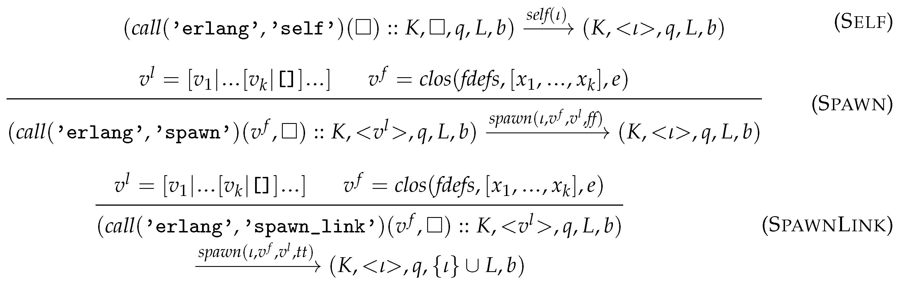
  • Rule Self reduces to the PID of the current process which is obtained from the inter-process level in the action self .
  • Rules Spawn and SpawnLink describe process spawning. The spawned process will evaluate the given function applied to the given parameters, which are communicated to it within the spawn action. To be able to evaluate this function application, the parameters of spawn are required to be a closure and a proper Core Erlang list. The result is the PID of the spawned process which is obtained from the inter-process semantics in the spawn action. In the case of rule SpawnLink, the flag in the spawn action is also set, and a link is established to the spawned PID.
Finally, we describe rules about process-local steps (Figure 11). Unlike in previous work [10,12,16], we express rules about message receipts with primitive operations; since receive expressions have been removed from the primitives of Core Erlang in OTP 23 [19], they are automatically expanded to the primitive operations.
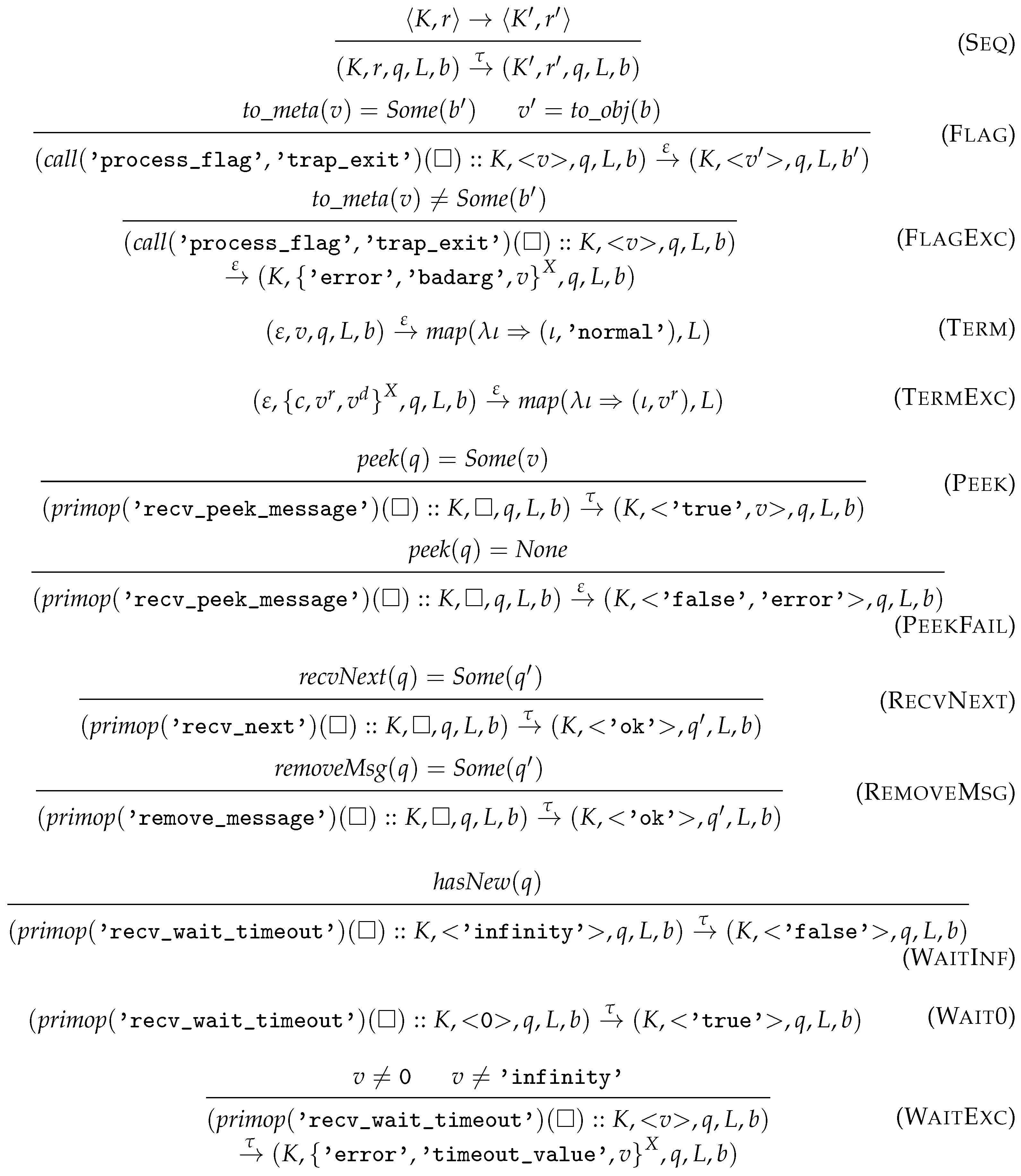
  • Rule Seq lifts the sequential steps to the process-local level.
  • Rule Flag changes the state of the trap_exit flag of the process to the provided boolean value, and its result is the original value of the flag. Rule FlagExc raises an exception, if a non-boolean value was provided.
  • Rule Term describes the normal termination. The links are notified with exit signals with ‘normal’ reason.
  • Rule TermExc describes the behaviour when an exception terminates the process. Each linked process is notified with an exit signal which includes the exception’s reason.
  • Rule Peek checks the first unseen message (if it exists). The result is a value sequence consisting of ‘true’ and the said message.
  • Rule PeekFail is used if there are no unseen messages in the mailbox. The result is a value sequence consisting of ‘false’ and an error value (which can be neither observed in the implementations, nor in the generated BEAM code).
  • Rule RecvNext moves the first unseen message into the list of seen messages (if it exists).
  • Rule RemoveMsg removes the first unseen message from the mailbox and sets all messages as unseen hereafter.
  • Rule WaitInf describes the semantics of unblocking. This rule is used if there is an unseen message, otherwise the process is blocked until one arrives. The result ‘false’ indicates that the timeout (‘infinity’) was not reached.
  • Rule Wait0 always evaluates to ‘true’, indicating that a timeout was reached. Currently, we have not formalised the timing; thus, only 0 and ‘infinity’ timeouts are modelled; however, we plan to change this in the future.
  • Rule WaitExc evaluates to an exception when an invalid timeout value (i.e., non-integer and non-infinity) was used.

3.5. Inter-Process Semantics

After having the process-local semantics defined, we turn our attention to the inter-process (node-level) semantics, which defines how actions should be propagated among processes. The main advantage of this semantics is its simplicity—it is described with only four rules. First, we define the notion of process pools.
Definition 4 
(Process pool). A (process) pool Π is a finite map (associative list) which assigns PIDs to processes.
In (Core) Erlang, signal passing is not atomic. According to the reference manual [9] “The amount of time that passes between the time a signal is sent and the arrival of the signal at the destination is unspecified but positive”; thus, we need to store these signals in an ether until they arrive. Moreover, this ether should respect the signal-ordering, i.e., “if an entity sends multiple signals to the same destination entity, the order is preserved” [9].
Definition 5 
(Ether). An ether is a finite map (associative list) which assigns a pair of PIDs (representing the source and destination of signals) to a list of signals. We denote ethers with Δ.
Definition 6 
(Node). A Core Erlang node N is a pair of a process pool and an ether. We use N Π and N Δ for the pool and ether of N.
Before discussing the four rules of the inter-process semantics, we introduce a number of notations for ethers and process pools.
  • ι : p Π denotes the pool consisting of process p (associated with PID ι ) and pool Π .
  • Δ [ ( ι s , ι d ) l ] updates the ether Δ by binding the pair of PIDs ( ι s , ι d ) to the list of signals l.
  • Δ [ ( ι s , ι d ) + s ] appends a signal s to the end of the list associated with ( ι s , ι d ) in the ether Δ . If there is nothing associated with the given source and destination, this function creates a singleton list associated with the given PIDs.
  • remFirst ( Δ , ι s , ι d ) removes the first signal from the list associated with ( ι s , ι d ) from Δ . Its result is of option type, if there is a signal to remove, the result is this signal and the modified ether enclosed in Some , otherwise None .
  • PIDsOf ( Δ ) and PIDsOf ( Π ) denote the PIDs that appear in Δ or Π , respectively. A PID appears in an ether if it is used as a source or destination of a signal, or if it appears syntactically in one of the signals stored in the ether. Respectively, a PID appears in a pool if there is a process associated with it, or it appears inside a process syntactically.
  • eval ( v f , v 1 , , v k ) notation is taken from [11]; here, we only use it to express beta-reduction of v f with the parameters v 1 , , v k . For more details, refer to Appendix A and [11].
Next, we discuss the semantics rules (shown in Figure 12). In general, all rules propagate an action to one of the processes inside the process pool, potentially changing the ether or creating new processes.
Remark 1. 
The rules of the inter-process semantics are decorated with a set of PIDs O; these PIDs are considered as observed, and no processes can be spawned on them. The communication to the PIDs in O is used to express the observable behaviour in bisimulation definitions in Section 4.
  • Rule NSend describes signal sending. When a process (associated with ι s ) sends a signal to ι d , this signal is placed into the ether with the source ι s and destination ι d .
  • Rule NArrive removes the first signal from the ether (with some source ι s ) to deliver to the process with PID ι d .
  • Rule NSpawn describes process creation. When a process reduces with a spawn action, the inter-process semantics assigns a fresh and unobserved PID ι 2 to the new process which will evaluate the given closure applied to the given parameters of the spawn action. If the flag in the spawn action is set (i.e., spawn_link has been evaluated in the process), a link to the parent process is also established. Whether v f is a closure and the third parameter of spawn is a proper Core Erlang list of values are checked in the process-local semantics (in rules Spawn and SpawnLink).
  • Rule NLocal defines that every other action should be only propagated to the process-local level without modifying the ether, or creating new processes.
We use N O * l N to denote the reflexive transitive closure of the semantics, where l is the evaluation trace of PID-action pairs. We write N O * a N if the trace only consists of actions a (and its length is irrelevant), and omit the trace entirely if it is not relevant.

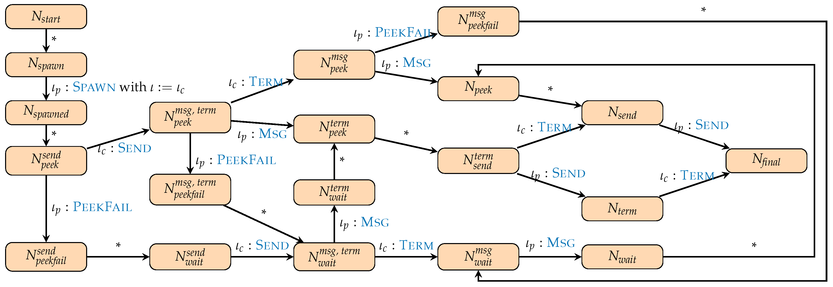
3.6. Example Evaluation

In this section, we show example evaluations for our running example presented in Figure 4, where we instantiate the metavariables in the following way (we keep ι as arbitrary):
e l : = [ 1 | [ 2 | [ 3 | [ 4 | [ ] ] ] ] ] i : = 2 e f : = fun ( X ) call   erlang : + ( X , 1 )
We remind the reader that the closure of the sequential list processing ( c map evaluated as the result closure of the letrec expression in Figure 3) is already substituted correctly.
Example 1 
(Concurrent map evaluation). We use the following shorthands for the evaluation. We note that we also labelled the code presented in Figure 2, Figure 3 and Figure 4 with the following shorthands to ease understanding.
  • e pmap 
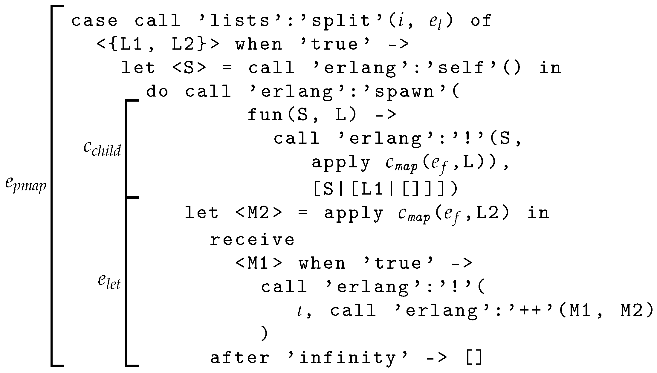
denotes the expression presented in Figure 4;
  • c child denotes the closure for the spawned process:
    clos ( , [ S , L ] , call erlang : ! ( S , apply c map ( e f , L ) ) ) ;
  • e let denotes the second subexpression of the  do  expression from Figure 4, which processes the list suffix sequentially, and receives the result from the child process;
  • e case denotes the outermost  case  expression (checking the result of peeking the mailbox) from Figure 2 substituted with the two cases of the  receive  expression in Figure 4;
  • e reccase denotes the innermost  case  expression (substituted with the concrete values in the  receive  expression of Figure 4) from Figure 2 which checks the result of the timeout;
  • cl 1 , cl 2 denote the clauses of the  case  expression of Figure 3.
  • v l is used for the transformed list [2|[3|[4|[5|[]]]]], and  v 1 l for the transformed prefix [2|[3|[]]].
Next, we present multiple ways to evaluate concurrent list transformation. For brevity, we show the sequential configurations, since the set of linked processes and the process flag does not influence this evaluation (i.e., they can be arbitrary for both the parent and the child process), and show the mailbox separately. First, we show the configurations for the parent in which a non-silent reduction can happen or happened, and the initial state:
ε , e pmap ( p start ) call ( erlang , spawn ) ( c child , ) : : do e let : : ε , [ 1 | [ 2 | [ ] ] ] ( p spawn ) do e let : : ε , < ι c > ( p do ) primop ( recv _ peek _ message ) ( ) : : : : let < Success , Msg > = in e case : : ε , ( p peek ) let < Success , Msg > = in e case : : ε , < false , error > ( p fail ) primop ( recv _ wait _ timeout ) ( ) : : : : let = in e reccase : : ε , < infinity > ( p wait ) call ( erlang , ! ) ( ι , ) : : ε , < [ 2 | [ 3 | [ 4 | [ 5 | [ ] ] ] ] ] > ( p send ) ε , < [ 2 | [ 3 | [ 4 | [ 5 | [ ] ] ] ] ] > ( p final )
The child process can also be in three such states where non-silent actions can happen. We present these and the child’s initial state:
ε , case [ 1 | [ 2 | [ ] ] ] of cl 1 ; cl 2 end ( c start ) call ( erlang , ! ) ( ι p , ) : : ε , < v 1 l > ( c send ) ε , < v 1 l > ( c final ) ( c term )
We highlight possible execution paths for the concurrent list transforming function. In Figure 13, we show the decision points where it matters which action to evaluate first. The semantics is strongly confluent for silent actions according to Theorems 3 and 4; thus, the order of silent reductions does not matter. For this reason, we do not discuss these steps (but refer to Appendix B for an example). In Figure 13, we use the notations below for the states of the node and denote silent reduction chains with (*). In the following list of pairs, the first component denotes the ether, the second the process pool consisting of at most the parent and child process, and the parent’s mailbox is explicitly described (the child’s mailbox is empty in all steps). The node’s subscripts highlight the next BIF that the parent has to evaluate, while the superscripts denote the remaining actions that can happen in the given configuration.
  • N s t a r t = ( , ( p s t a r t , [ ] ))
  • N s p a w n = ( , ( p s p a w n , [ ] ) )
  • N s p a w n a f t e r = ( , ( p d o , [ ] ) c s t a r t )
  • N p e e k s e n d = ( , ( p p e e k , [ ] ) c s e n d )
  • N p e e k f a i l s e n d = ( , ( p f a i l , [ ] ) c s e n d )
  • N p e e k m s g , t e r m = ( [ ( ι c , ι p ) + v 1 l ] , ( p p e e k , [ ] ) c f i n a l )
  • N p e e k f a i l m s g , t e r m = ( [ ( ι c , ι p ) + v 1 l ] , ( p f a i l , [ ] ) c f i n a l )
  • N w a i t s e n d = ( , ( p w a i t , [ ] ) c s e n d )
  • N p e e k f a i l m s g = ( [ ( ι c , ι p ) + v 1 l ] , ( p f a i l , [ ] ) c t e r m )
  • N p e e k m s g = ( [ ( ι c , ι p ) + v 1 l ] , ( p p e e k , [ ] ) c t e r m )
  • N p e e k t e r m = ( , ( p p e e k , [ v 1 l ] ) c f i n a l )
  • N w a i t t e r m = ( , ( p w a i t , [ v 1 l ] ) c f i n a l )
  • N w a i t m s g , t e r m = ( [ ( ι c , ι p ) + v 1 l ] , ( p w a i t , [ ] ) c f i n a l )
  • N p e e k = ( , ( p p e e k , [ v 1 l ] ) c t e r m )
  • N s e n d t e r m = ( , ( p s e n d , [ ] ) c t e r m )
  • N w a i t m s g = ( [ ( ι c , ι p ) + v 1 l ] , ( ( p w a i t , [ ] ) c t e r m )
  • N s e n d = ( , ( p s e n d , [ ] ) c t e r m )
  • N t e r m = ( [ ( ι p , ι ) + v l ] , ( p f i n a l , [ ] ) c t e r m )
  • N w a i t = ( , ( p w a i t , [ v 1 l ] ) c f i n a l )
  • N f i n a l = ( [ ( ι p , ι ) + v l ] , p f i n a l , [ ] ) c f i n a l )
The evaluation starts with the parent splitting the list in half (since i = 2 ), and spawning the child process ( N s t a r t , N s p a w n , N s p a w n e d ). Next, both the parent and child process evaluate the map function sequentially for their list segments reaching N p e e k s e n d (for this evaluation, we refer to Appendix B, Example A1). At this point, either the child sends its result to the parent, or the parent fails to evaluate‘recv_peek_message’. Actually, the child can even send the message ( N p e e k f a i l m s g , t e r m ), and terminate ( N p e e k f a i l m s g ), while the parent still fails on‘recv_peek_message’, because the message has not been delivered yet (with Msg).
If the parent failed in either of the previous steps, it becomes stuck on an infinite timeout, until the message from the child arrives. Next, the parent continues the evaluation of the message receipt recursively (see Figure 2), and retries peeking into the mailbox. This leads to N p e e k t e r m (if the child is not yet terminated) or N p e e k (if the child is already terminated). If the parent tried peeking into the mailbox only after the message had arrived (i.e., peeking had never failed), then one of the previous two states was reached, too.
Finally, the parent successfully receives the transformed list from the child (reaching either N s e n d t e r m or N s e n d ); then it appends the two segments and sends the result to the observed PID ι.

3.7. Semantic Properties

Next, we show a number of properties of the concurrent semantics, and for their proofs, we refer to the formalisation [29], and to Appendix C, which connects the concepts of this paper, to the code. First, we state that our semantics respects the signal ordering guarantee [9].
Theorem 1 
(Signal ordering guarantee). For all nodes N 1 , N 2 , N 3 , PIDs ι , ι , and unique signals (i.e., they are different from any other signal in the starting configuration). s 1 s 2 , if  N 1 ι : send ( ι , ι , s 1 ) O N 2 and N 2 ι : send ( ι , ι , s 2 ) O N 3 , then for all nodes N 4 and action traces l which satisfy N 3 O * l N 4 and also ( ι , arr ( ι , ι , s 1 ) ) l then N 5 : N 4 ι : arr ( ι , ι , s 2 ) O N 5 (i.e., there is no node at which s 2 can arrive).
To reason about process creation in later sections, it is inevitable to reason about PID renaming. We use renaming when arguing about process spawns because in most cases, the freshness criteria imposed by NSpawn is too weak as it depends only on O and the node the spawn is evaluated in. In some cases, there could be other PIDs that should be distinct from the spawned one (e.g., when reasoning about node equivalence).
Definition 7 
(PID renaming). We denote PID renaming with r [ ι 1 ι 2 ] , which syntactically replaces all occurrences of ι 1 with ι 2 inside a redex r. For simplicity, we use the same notation for frame stacks, mailboxes, lists, and live processes.
We denote PID renaming for finite maps (dead processes, ethers, process pools, and nodes) with N [ ι 1 ι 2 ] . For these syntactical constructs, renaming is the syntactical exchange of the given two PIDs. With this notion, we avoid accidental overwriting of existing bindings in a finite map.
Given a list of PID pairs [ ( ι 1 , ι 1 ) , , ( ι n , ι n ) ] , we use r [ ι 1 ι 1 , , ι n ι n ] (and N [ ι 1 ι 1 , , ι n ι n ] ) for sequential renaming, i.e.,  r [ ι 1 ι 1 ] [ ι n ι n ] ( N [ ι 1 ι 1 ] [ ι n ι n ] , respectively).
PIDs cannot be renamed freely while reasoning about program equivalence; we have to make sure that we do not bind observed or used PIDs while renaming. This property is expressed with the following two compatibility definitions. Node-compatibility ensures that a renaming satisfies the freshness conditions, and action-compatibility ensures that this freshness condition is respected by the reductions with the given actions.
Definition 8 
(Node-compatible renaming). A list of PID pairs [ ( ι 1 , ι 1 ) , , ( ι n , ι n ) ] is compatible with a node N and observable PIDs O, if for all indices i the following points are all satisfied:
  • ι i , ι i O ;
  • ι i PIDsOf ( N Δ [ ι 1 ι 1 , , ι i 1 ι i 1 ] ) ;
  • ι i PIDsOf ( N Π [ ι 1 ι 1 , , ι i 1 ι i 1 ] ) .
Definition 9 
(Action-compatible renaming). A list of PID pairs [ ( ι 1 , ι 1 ) , , ( ι n , ι n ) ] is compatible with an action a, if for all indices i, ι i PIDsOf ( a [ ι 1 ι 1 , , ι i 1 ι i 1 ] ) .
We note that we can always define a compatible renaming for a node or action based on fresh PIDs. Next, we show that node and action-compatible renamings preserve the semantics.
Theorem 2 
(Renaming preserves reduction). For all lists of PID pairs [ ( ι 1 , ι 1 ) , , ( ι n , ι n ) ] which are compatible with nodes N with observable PIDs O, and actions a, all reductions N ι : a O N are preserved by the compatible renaming, i.e.,
N [ ι 1 ι 1 , , ι n ι n ] ι [ ι 1 ι 1 , , ι n ι n ] : a [ ι 1 ι 1 , , ι n ι n ] O N [ ι 1 ι 1 , , ι n ι n ] .
In addition to renaming, the other important property of the semantics is confluence, on which some of our equivalence examples depend. We proved two confluence properties: a diamond property for reasoning about different processes, and a strong confluence property for reasoning about silent actions. For the first theorem, we need to define the compatibility of actions.
Definition 10 
(Compatibility between actions). Two actions are compatible, if neither of them is a spawn action, or if one is a spawn ( ι , v 1 , v 2 , b ) action, the other one is not spawn ( ι , v 3 , v 4 , b ) or send ( ι s , ι , v ) (i.e., in case of spawn or send, the used (and target) PIDs are different).
The previous definition can always be satisfied by using PID renaming for the spawn actions.
Theorem 3 
(Commutativity of reductions (a restricted diamond property)). For all nodes N 1 , N 2 , N 2 , compatible actions a 1 , a 2 , and PIDs ι 1 ι 2 , if  N 1 ι 1 : a 1 O N 2 and N 1 ι 2 : a 2 O N 2 , there exists a node N 3 , which satisfies both N 2 ι 2 : a 2 O N 3 and N 2 ι 1 : a 1 O N 3 .
Theorem 4 
(Strong confluence with silent actions). For all nodes N 1 , N 2 , N 2 , silent actions a s , actions a, and PIDs ι, if  N 1 ι : a s O N 2 and N 1 ι : a O N 2 , then one of the following cases is satisfied:
  • a s = a and N 2 = N 2 ; or
  • a is an arrive action, there is a node N 3 , such that N 2 ι : a O N 3 , and either N 2 ι : a s O N 3 or N 3 = N 2 (in the latter case, the process with PID ι was terminated).

4. Program Equivalence

In this section, we investigate a number of definitions for program equivalence based on barbed bisimulation [30]. This section is structured as follows. In Section 4.1, we introduce the usual notion of strong and weak (barbed) bisimulations, and argue why they are insufficient to reason about (Core) Erlang nodes. Next, in Section 4.2, we introduce a refined program equivalence concept based on barbed bisimulation, which is suitable to argue about refactoring correctness on concurrent programs. Finally, in Section 4.3, we enumerate a number of bisimulation examples which can be considered as correct concurrent refactorings.

4.1. Restrictive Notions of Program Equivalence

Practically, two concurrent programs are equivalent, if an external observer cannot distinguish their behaviour. For us, the communication (i.e., the signals sent) of a node can be observed from the outside. For barbed bisimulations, we have to characterise this property. First, we define the observable behaviour as the signals in a node’s ether targeting some PID in the set O (i.e., O is the observer, and the signals sent to it define the observed behaviour). Based on this thought, we can define when two nodes agree on the observed signals:
Definition 11 
(Nodes agree on observed signals). Two nodes N 1 , N 2 weakly agree on O, when for all PIDs ι s , ι d , if  ι d O implies that there exists a PID ι 2 s such that N 1 Δ [ ( ι s , ι d ) ] N 2 Δ [ ( ι 2 s , ι d ) ] , where ≃ denotes syntactical equality up to PIDs.
Two nodes strongly agree on O, if they weakly agree on O; moreover, ι 2 s = ι s in the previous definition.
The first definition we investigate is barbed strong bisimulation, which relates two nodes whenever they can make the same reductions, and they agree on the signals sent to observed PIDs.
Definition 12 
(Barbed strong bisimulation). A relation R on nodes is a barbed strong bisimulation observing O if given two nodes N 1 , N 2 , R ( N 1 , N 2 ) implies the following:
  • For all nodes N 1 , actions a, and PIDs ι, if  N 1 ι : a O N 1 then N 2 : N 2 ι : a O N 2 and R ( N 1 , N 2 ) ;
  • The converse of the previous point for reductions from N 2 ;
  • N 1 and N 2 strongly agree on O (note that this property is symmetric).
We use N 1 O N 2 to denote that N 1 and N 2 are related by a relation R which is a barbed strong bisimulation.
Proving strong bisimilarity even between simple nodes is impossible in most practical cases. Consider a node consisting of one process which computes the expression call erlang : + ( 1 , 2 ) and a node with a process computing 3 . The first node can take some τ computation steps, which could not be taken by the second one. To loosen this notion of program equivalence, we can introduce weak bisimulations.
Definition 13 
(Barbed weak bisimulation). A relation R on nodes is a weak barbed bisimulation observing O if given two nodes N 1 , N 2 , R ( N 1 , N 2 ) implies the following:
  • For all nodes N 1 , actions a, and PIDs ι, if  N 1 ι : a O N 1 then N 2 , N 2 , N 2 : N 2 O * τ N 2 O ι : a N 2 O * τ N 2 and R ( N 1 , N 2 ) ;
  • The converse of the previous point for reductions from N 2 ;
  • N 1 and N 2 strongly agree on O.
We use N 1 O N 2 to denote that N 1 and N 2 are related by a relation R which is a weak barbed bisimulation.
Remark 2. 
There is no need to include silent reduction steps from N 2 in the third point of Definition 13 as τ actions do not affect the ether.
With this definition, we can prove examples like the previous one, which only differ in computational steps, but cannot prove equivalence between nodes that communicate or spawn processes differently. In particular, with this notion, we cannot prove the equivalence between the two list processing functions from the running example (Figure 3 and Figure 4). This is because the sequential variant only communicates the result of the computation, while the parallel version spawns a child process and also performs communication between the child and parent processes.

4.2. Alternative Notion for Weak Barbed Bisimulation

We borrow another idea of (weak) barbed bisimulation used for related research on Core Erlang [16], and tailor it to our needs. In this definition, we do not compare the actions that induce the reductions made by the nodes, and only focus on the observables. If a reduction is taken by one node, the other one has to simulate it, but there is no restriction on what and how many steps this simulation should take.
Definition 14 
(Barbed bisimulation). A relation R on nodes is a barbed bisimulation observing O, if given two nodes N 1 , N 2 , R ( N 1 , N 2 ) implies the following:
  • For all nodes N 1 , actions a, and PIDs ι, if  N 1 ι : a O N 1 then N 2 : N 2 O * τ N 2 and R ( N 1 , N 2 ) ;
  • N 2 : N 2 O * τ N 2 and N 1 and N 2 weakly agree on O;
  • The converse of the previous points for reductions and observables of N 2 .
We use N 1 O N 2 to denote that N 1 and N 2 are related by a relation R which is a barbed bisimulation. Hereafter, whenever we write bisimulation, we mean this definition.
After defining the suitable notion of program equivalence, we state the basic properties of this relation: reflexivity, symmetry, and transitivity. We furthermore highlight that this notion is less restrictive than the previous two definitions (for the proofs, refer to the formalisation [29]).
Theorem 5 
(Equivalence relation). For all sets of PIDs O, the relation O is reflexive, symmetric, and transitive.
Theorem 6 
(Correspondence between bisimulations). For all sets of PIDs O, O O O .

4.3. Bisimulation Examples

Next, we show some bisimilar node pairs. For complete proofs, we refer to the formalisation [29], while we also give some insights here. In general, to prove these lemmas, we relied on coinduction, and case distinction based on the four rules of the inter-process semantics (Figure 12). To reason about spawn actions, in most cases, we also had to use renaming (either with Theorem 7 or with the coinductive hypothesis).
Theorem 7 
(PID-renaming is a barbed bisimulation). For all lists [ ( ι 1 , ι 1 ) , , ( ι n , ι n ) ] containing PID pairs which are compatible with the node N and sets of PIDs O, N O N [ ι 1 ι 1 , , ι n ι n ] .
Proof. 
We proceed with coinduction. We need to prove the four conditions of the bisimulation (Definition 14). The proof of the third and fourth points is based on the symmetric properties of bisimulations, and equality; thus, we only briefly explain the proof of the first two points. For readability, we use l to denote the list of renamings ι 1 ι 1 , , ι n ι n (or ι 1 ι 1 , , ι n ι n depending on the context).
Suppose that N ι : a O N . We need to show N [ l ] ι [ l ] : a [ l ] O N [ l ] . According to Theorem 2, if the renaming is compatible with action a, we can show that the renaming preserves the reduction, and by the coinductive hypothesis, the reached nodes are bisimilar. Since the renaming is compatible with the initial node, it is also compatible with almost all actions, because the PIDs that appear in the actions originated either from the ether or the process pool. On the other hand, spawn actions involve a fresh PID ( ι s p a w n ), which could collide with the PIDs used for renaming. In this case, we can extend the list of renamings with a new renaming: ( ι s p a w n , ι f r e s h ) : : l . Since ι f r e s h is chosen arbitrarily, we can ensure that it does not appear in the node or the action, and this extended list is compatible with action a, thus N [ ι s p a w n ι f r e s h , l ] ι [ ι s p a w n ι f r e s h , l ] : a [ ι s p a w n ι f r e s h , l ] O N [ ι s p a w n ι f r e s h , l ] , and we can use the coinductive hypothesis for this extended list to prove that the reached nodes are bisimilar.
The proof of the second point is mostly technical. If there are signals targeting ι d O in the ether of N (e.g., with the source ι s ), we can show that there are signals targeting ι d in N [ l ] too, with the source ι s [ l ] . Moreover, these signals are equal up to the PIDs.    □
While PID renaming seems to be an obvious (and often implicitly used) property, in a machine-checked formalisation, we need to be rigorous and explicit both in its proof and in its uses. Without renaming, there is no way to reason about nodes that use different PIDs, and also spawn some new processes, since the spawned PID is potentially not fresh in the other node. We mitigate this problem by renaming the spawned PID to a fresh(er) one.
Next, we state two technical lemmas to reason about elements of the ether and process pool which do not affect the evaluation. With these lemmas, we can remove irrelevant signals and terminated processes from a node during bisimulation proofs. The first lemma states that signals originating from, or targeting, terminated processes do not distinguish nodes.
Lemma 1 
(Ether update for terminated processes). For all nodes N, sets of PIDs O, and PIDs ι s , ι d which satisfies ι d O , if both N Π [ ι s ] and N Π [ ι d ] are terminated processes, then for any list of signals l, N O ( N Δ [ ( ι s , ι d ) l ] , N Π ) , and  N O ( N Δ ( ι s , ι d ) , N Π ) .
Proof. 
We proceed by coinduction. We need to prove the four conditions of the bisimulation (Definition 14). The points about observables trivially hold since the update in the ether does not affect observed PIDs.
Suppose that N ι : a O N , then we have to show that we can perform an equivalent step with the updated ether.
  • If NLocal or NArrive was used, then the same step can be made in the updated node (since these actions could not have been taken by terminated processes), and we can use the coinductive hypothesis.
  • If NSpawn was used (which could not have been performed by a terminated process), we have to rename the PID of the spawned process to a fresh PID (so that it does not appear anywhere in the modified configuration, nor in the set of PIDs used in l), and we can perform the same reduction step with the fresh PID, since it satisfies the side condition of NSpawn. We finish this case by using the transitivity of barbed bisimulation with Theorem 7 and the coinductive hypothesis.
  • In the case of NSend, we can make the same reduction in the updated node, regardless of which process sent the message. Supposing that a = send ( ι s , ι d , s ) , we can use the coinductive hypothesis with the list of signals chosen as l + + [ s ] (or just [ s ] , if we prove the second part of the theorem).
For the converse direction, we can use the fact that any ether E can be expressed with two updates:
  • If E [ ( ι s , ι d ) ] = Some ( l ) , then E = E [ ( ι s , ι d ) l ] [ ( ι s , ι d ) l ] .
  • If E [ ( ι s , ι d ) ] = None , then E = E [ ( ι s , ι d ) l ] ( ι s , ι d ) .
Therefore, we can use the same train of thought as described above to conclude the proof.    □
The following lemma states that adding unlinked terminated processes (we denote empty maps with ) to a node creates an equivalent node.
Lemma 2 
(Terminated process). For all nodes N, sets of PIDs O, and PIDs ι, if  ι O and ι dom ( N Π ) , then N O ( N Δ , ι N Π ) .
Proof. 
This proof is also constructed with coinduction. The main idea is that the terminated process cannot take any reduction; thus, the same reductions can be made in both nodes, and this way, the ether is not affected either (i.e., observables remain the same).    □
The next theorem states that if a node can be reduced with τ steps or self actions, the result is equivalent to the original node. It is useful to reason about concrete node equivalences since it reduces the problem of proving bisimulation to proving evaluation. Together with the transitivity of O , in bisimulation proofs, we can discharge reasoning about silent steps.
Theorem 8 
(Silent evaluation). For all nodes N , N , sets of PIDs O, if  N O * l N for some action trace l, which contains only silent (i.e., τ or self ) actions, N O N holds.
Proof. 
For this theorem, it is sufficient to prove that one single silent step creates bisimilar nodes, since based on this fact and the transitivity of the barbed bisimulation (Theorem 5), we can prove the original property by induction on the action trace l.
To prove that a single silent step creates bisimilar nodes, we use coinduction, and prove the four requirements for barbed bisimulation. Suppose that a = τ ι , a = self ( ι ) , and  N ι : a O N . We prove N O N : .
First, we check what other possible reductions can be made from N based on the first point in Definition 14. Suppose that for some action a , PID ι and node N , there is a reduction N ι : a O N . We have to show that
N f i n a l , N O * N f i n a l N O N f i n a l .
There are the following options:
  • If ι = ι , then there are two options:
    -
    If a = a , i.e., the same step is taken, then N = N and we can choose N f i n a l = N and use the reflexivity of the bisimulation.
    -
    If a a , then a can only be an arrive action (Theorem 4). Supposing that the arrive action does not terminate the process, it can be postponed after making the reduction with a; thus, there is a node N to which N ι : a O N and N ι : a O N . We choose N f i n a l = N , which is reachable from N based on the first reduction, and prove N O N based on the coinductive hypothesis and the second reduction.
    -
    If a a , a is an arrive action, and it terminates the process, then the process is also if the action arrives in N , since silent actions do not modify either of the properties (linked PIDs, source and destination, exit reason, process flag) used in the semantics for arrives (see Figure 8); thus, N ι : a O N . We can choose N f i n a l = N and use the reflexivity of the bisimulation.
  • If for some action a , PID ι and node N , there is a reduction N ι : a O N , then we can use Theorem 3 to derive the existence of a node N to which N ι : a O N and N ι : a O N . We choose N f i n a l = N , which is reachable from N based on the first reduction, and prove N O N based on the coinductive hypothesis and the second reduction.
To prove that for all reductions N ι : a O N , the result N is bisimilar to a node which is reachable from N, we can chain this reduction after the assumption of N ι : a O N , and use the reflexivity of the bisimulation (Theorem 5).
The observables are not modified in the ether by silent actions; thus, the requirements on them of Definition 14 hold.    □
We highlight that this theorem is more restrictive than the normalisation theorem of [16], which also considers message sending and process spawning in this bisimulation (we refer the reader to Section 5 for a discussion of why this is not the case for us). Finally, we show a concrete program equivalence based on barbed bisimulation.
Example 2 
(Equivalence of sequential and concurrent map).  Consider the expressions from Figure 3 (denoted with e map ) and Figure 4 (denoted with e pmap ). For all values v l , v f , natural numbers i, PIDs ι which appear as the metavariables in Figure 3 and Figure 4, and for all PIDs ι b a s e , ( , ι b a s e ( ε , e map , [ ] , , ff ) ) { ι } ( , ι b a s e ( ε , e pmap , [ ] , , ff ) ) , if the following conditions hold:
  • ι b a s e ι .
  • The closure value v f computes a metatheoretical function f, that is, for all values v, we can prove ε , apply v f ( v ) * < f ( v ) > in the sequential layer.
  • v l is a proper Core Erlang list, i.e., it is constructed as [ v 1 | [ v 2 | [ v n | [ ] ] ] ] , and  i n .
  • v l does not contain any PIDs; moreover, the application of v f does not introduce any PIDs.
Proof Sketch. 
The proof of this theorem is quite involved; thus, we refer to the formalisation [29] for all details, and only describe the main idea here. We avoided using the definition of the bisimulation manually since it takes many reductions to evaluate both sequential and parallel list transformation, and reasoning about the four conditions of Definition 14 generates unnecessary, tremendous overhead. Instead, we heavily rely on Theorem 8 and the transitivity of bisimulation (Theorem 5) to discharge silent evaluation steps from the reasoning.
There are two main points to prove: there is an evaluation of the parallel list processing that behaves the same way as the sequential one, and vice versa. The former point follows from the fact that the sequential map can be only evaluated deterministically (see Example A1 for more insights) and from Example 1 where (all) paths lead to the same final configuration. The latter point is more challenging, since all evaluation paths in Figure 13 have to be simulated by the sequential list processing. To prove this, we need to manually apply the definition of bisimulation in all states from Figure 13 from where a non-silent reduction happens.    □

5. Discussion

In this section, we describe the novelty of this work with respect to our previous work we build on. We also discuss some major theoretical and technical challenges originating from the formalised signals, the absence of atomic receive expressions, and the fact that our formalisation is mechanized in Coq.

5.1. Novelty

As mentioned before, this paper builds on, and extends, our previous work described in [10,11]. Namely, we reused the sequential semantics of [11] (which we recall in Appendix A), and built the process-local and inter-process semantics on top of it based on [10]. However, note that we do not repeat the definitions presented there; in particular, this current paper not only extends our previous work but defines the communication primitives with a different granularity (i.e., with the new primitives implemented in Erlang/OTP version 23 [19]), which required changes in the underlying representations compared to [10] (such as that of mailboxes, process pools, and the ether), the semantic rules, and the proofs of the fundamental properties. Since the implementation of the new communication primitives does not fully conform with the old language specification, our work is essential, and it sets the state-of-the-art regarding the formal definition of the actor model of Erlang, providing a rigorous and solid basis for future research on the most recent communication model.

5.2. Theoretical Challenges

The first challenge we encountered was the definition of the inter-process semantics, which had to satisfy both the signal-ordering guarantee and the fact that message passing is not atomic (as explained in Section 3.5). These conditions make it necessary to define an ether that includes the sent but not delivered signals in an ordered way. In addition to making the semantics more complex, this decision also makes some reductions impossible, which would have been carried out if the signal-ordering guarantee was not enforced. On the other hand, this simplifies reasoning about signal arrival, since only the first signals need to be considered from the ether (from the ordered list of signals) targeting a process.
Next, the formalisation of exit signals comes with a number of challenges. Since exit signals can potentially terminate a process, they also limit the confluence properties of the semantics. This is also one of the reasons why Theorem 8 is more restricted than “normalisation” (from [16]) which also allows send and ε actions in the reduction chain. Whether an exit signal terminates a process depends on a number of factors: which are the linked PIDs, how the trap_exit flag is set, what is the reason value, and the source of the signal. If the process for which the exit is arriving can also make a step which modifies either of these, the process will behave in a different way if the signal arrives before or after this step, and this breaks the confluence property.
A similar argument can be made about the correlation between primitive operations for message receipts and arrival. For example, if a message arrives before evaluating recv_peek_message, then the first component of its result is the atom true , while if the message arrives later, the same component could be ‘false’ (if there are no unseen messages in the mailbox). This means that Lemma 9 of [16]—saying that any reduction that can be made with a process can also be made if a new message is appended at the end of the mailbox—cannot be proved; this lemma only holds for receive expressions that evaluate in an atomic way. To handle the maximum number of reductions with Theorem 8 when reasoning about bisimulations, we decided to label all reductions with τ (not just steps of the sequential layer) for which the semantics is strongly confluent.

5.3. Formalisation

As mentioned before, all of our results are machine-checked with Coq [29] (around 35,000 lines of code). We briefly explain the main design decisions we made.
  • We deeply embedded the syntax of Core Erlang into Coq as an inductive definition, so that we can use induction to reason about substitutions, PID renamings, and variable scoping.
  • We encoded variables (and function identifiers) of Core Erlang with the nameless variable representation, i.e., all variables are de Bruijn indices. Using a nameless encoding simplifies reasoning about alpha-equivalence to checking equality, and fresh variable generation is simply expressed with addition of natural numbers. This way, the syntax is less readable for the human eye, but it is much simpler to define parallel capture-avoiding substitutions and use them in proofs [31].
  • We did not use a similar, nameless encoding for PIDs. While process pools behave like binders, PIDs generally do not behave as variables: PIDs are dynamically created, and we do not apply substitutions for them. Moreover, in some cases, we might need to depend on the exact value of a PID in the program (e.g., for PID comparison). In addition, alpha-equivalence of PIDs cannot be reduced to equality checking with a nameless encoding. Suppose that we have several process spawns that can be executed in any order. After executing all process spawns in all possible orders, the result systems will be alpha-equivalent, but never equal, since the spawned PIDs (as de Bruijn indices) would depend on the particular execution path.
  • We expressed all semantic layers as inductive judgements in order so that we could more easily use Coq’s tactics (inversion and constructor) to handle semantic reductions in proofs.
  • We formalised process pools, ethers and dead processes as finite maps so that the used PIDs inside such constructs can be collected by a recursive function. Based on the collection result, we can come up with fresh PIDs for spawned processes. If we used functions instead of finite maps, showing that a concrete PID does not appear inside process of a process pool would have required much more complex proofs (potentially based on induction).
  • For an implementation of finite maps and freshness, we relied on the Iris project’s stdpp [32] library, which also includes the set_solver tactic that can be used to automatically discharge statements about sets and finite maps.
  • The formalisation depends only on one standard axiom; we use functional extensionality for reasoning about parallel substitutions.
Having a machine-checked formalisation also comes with some drawbacks. Firstly, a proof assistant forces the proof engineer to be more precise compared to writing mathematical proofs on paper. For our project, this creates technical difficulties whenever reasoning about spawn actions is needed, because (in most cases) at these steps, we have to rely on renaming with fresh PIDs. After defining the necessary fresh PIDs, we have to manually simplify these renamings, and in equivalence proofs, based on the transitivity of the bisimulation (Theorem 5), we use Theorem 7 to reach the desired results.
However, relying on the transitivity of the bisimulation (or any other bisimulation-transforming proof) comes with another drawback: in a coinductive proof, the guardedness checker of Coq does not accept proofs that use transitivity on the coinductive hypothesis, since it is often unsound (for now, we turned off the guardedness checker for these proofs and relied on existing approaches [16] to carry out the proofs; we intend to investigate other approaches to this). However, the violations of the guardedness only originate from the following two proof strategies.
  • In Theorem 7, we used bisimulation’s symmetry to justify the first clause of Definition 14 for the derivations starting from N 2 (i.e., for the node with renamings); however, we are certain that this could be replaced by several analogous helper lemmas, ultimately discharging the potential of invalidity.
  • For every other case (including Lemmas 1 and 2), we used bisimulation’s transitivity with Theorem 7 for injective alpha-renaming (based on the soundness results of [33]).

6. Conclusions and Future Work

We have defined formal semantics for the concurrent subset of Core Erlang, building on earlier work [10,11], extending the sequential syntax with process identifiers (PIDs), and defining the concurrent (process-local and inter-process) semantics by defining the meaning of concurrent built-in functions and primitive operations.
We defined three concepts of concurrent program equivalence based on barbed bisimulations. We argued that the usual notions of strong and weak bisimulations are too restrictive to reason about program equivalence. In order to model equivalence between programs that have different communication structure but the same observable behaviour, we introduced a weaker variant of barbed bisimulation (following the footsteps of [16,24]), with which we proved a number of program equivalences (such as PID renaming, executing computation steps, list processing sequentially or concurrently), reaching beyond previous and related work. The results presented here are formalised in the Coq proof assistant.
In the future, we aim to generalize the equivalence proof for sequential and concurrent list processing to include exit signals and message source validation. We then aim to generalize and create new approaches for reasoning about bisimulations to make it simpler to show concrete Core Erlang programs equivalent, to fulfil our goal of verifying Erlang refactorings.

Author Contributions

Conceptualization, P.B., D.H. and S.T.; funding acquisition, P.B. and D.H.; investigation, P.B.; methodology, P.B., D.H. and S.T.; project administration, D.H. and S.T.; software, P.B.; supervision, D.H. and S.T.; original draft, P.B.; Review and editing, P.B., D.H. and S.T. All authors have read and agreed to the published version of the manuscript.

Funding

This research was supported by the ÚNKP-23-3 New National Excellence Program of the Ministry for Culture and Innovation from the source of the National Research, Development and Innovation Fund. Project no. TKP2021-NVA-29 has been implemented with the support provided by the Ministry of Culture and Innovation of Hungary from the National Research, Development and Innovation Fund, financed under the TKP2021-NVA funding scheme.

Data Availability Statement

The original data presented in the study are openly available in [29].

Conflicts of Interest

The authors declare no conflicts of interest.

Appendix A. Rules of the Sequential Semantics

In this section, we recall the rules of the sequential semantics from our previous work [11]. The rules are categorised into four groups:
  • Rules that deconstruct an expression by extracting its first redex while putting the rest of the expression in the frame stack (Figure A1).
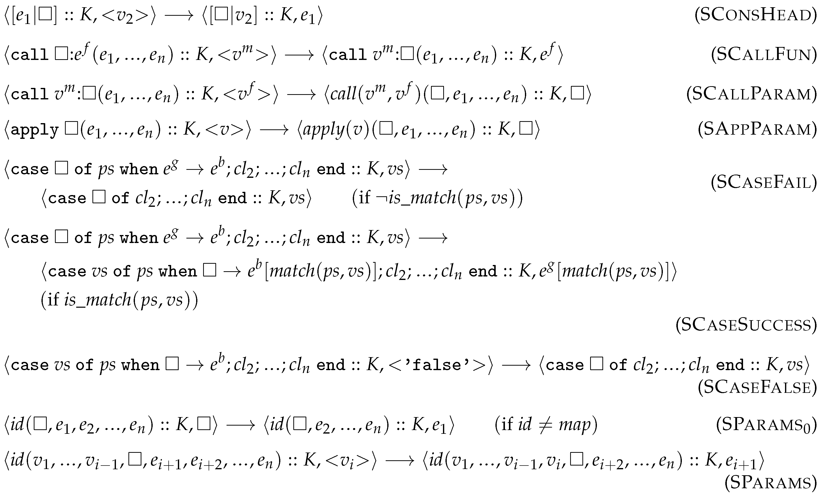
  • Rules that modify the top frame of the stack by extracting the next redex and putting back the currently evaluated value into this top frame (Figure A2).
  • Rules that remove the top frame of the stack and construct the next redex based on this removed frame (Figure A3). We also included rules here which immediately reduce an expression without modifying the stack (e.g., PFun).
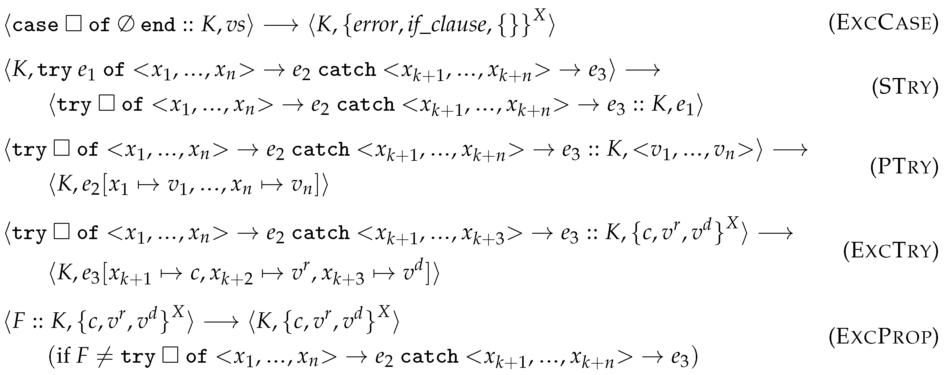
  • Rules that express concepts of exception creation, handling, or propagation (Figure A4).
Next, we recall some of the auxiliary definitions, which are necessary to understand the semantics rules.
  • r [ x 1 v 1 , , x n v n ] : substitutes names (variables or function identifiers) x 1 , , x n in the the redex r with the given values v 1 , , v n . In some cases, we use the same notation ( r [ l ] ) for substituting a list containing name–value pairs in the same way.
  • mk _ closlist ( fdefs ) : creates a list of function identifier–closure pairs from the list fdefs . Every function definition f / k = fun ( x 1 , , x k ) e in the list is mapped to the following pair in the result list: ( f / k , clos ( fdefs , [ x 1 , , x k ] , e ) ) .
  • is _ match ( ps , vs ) : decides whether a pattern list ps matches pairwise a value list vs (of the same length). A pattern matches a value, when they are constructed from the same elements, while pattern variables match every value.
  • match ( ps , vs ) : defines the variable-value binding (as a list of pairs) resulted by successfully matching the patterns ps with the values vs .
We provide an informal overview of eval ( id , v 1 , , v n ) here. If 
  • id = app ( v ) and v = clos ( fdefs , [ x 1 , , x n ] , e ) , then
    eval ( app ( v ) , v 1 , , v n ) = e [ mk _ closlist ( fdefs ) , x 1 v 1 , , x n v n ] .
  • id = app ( v ) and v is not a closure, or has an incorrect number of formal parameters, the result is an exception.
  • id = tuple , then eval ( tuple , v 1 , , v n ) = { v 1 , , v n } .
  • id = values , then eval ( values , v 1 , , v n ) = < v 1 , , v n > .
  • id = map and n is an even number, then
    eval ( map , v 1 , , v n ) = { v 1 v 2 , , v k 1 v k } ,
    where the k n result values inside the map are obtained by eliminating duplicate keys and their associated values.
  • id = call ( a m , a f ) , then eval ( call ( a m , a f ) , v 1 , , v n ) simulates the behaviour of sequential built-in functions of (Core) Erlang.
  • id = primop ( a ) , then eval ( primop ( a ) , v 1 , , v n ) simulates the behaviour of sequential primitive operations of Core Erlang.
We highlight a few points of this semantics but refer to [11] for all further details.
Figure A1. Frame stack semantics rules of 1.
Computers 13 00276 g0a1
Figure A2. Frame stack semantics rules of 2.
Computers 13 00276 g0a2
Figure A3. Frame stack semantics rules of group 3.
Computers 13 00276 g0a3
Figure A4. Frame stack semantics rules of group 4.
Computers 13 00276 g0a4

Appendix A.1. Parameter Lists

To avoid duplication of reduction rules for language elements involving parameter lists (value lists, tuples, maps, applications, inter-module calls, and primitive operations), we introduce parameter list frames Figure 5. These parameter lists are always evaluated in the same leftmost, innermost way, which is reflected in SParams. If there are no more parameters to evaluate, we finish the evaluation with PParams. Empty parameter lists are handled separately with PParams0 and SParams0, since if there are no parameters, there is no expression to be put into the second configuration cell of the semantics. This is also the reason, why □ is used as a redex in SAppParam, SCallParam, STuple, SPrimOp.

Appendix A.2. Map Frames

Maps are handled in a special way with parameter list frames. To ensure some semantic properties, we have to make sure that the number of values and expressions in a map parameter list frame is an odd number, so that together with the current redex, a valid map expression can be reconstructed. This is the reason why empty maps are handled separately with PMap0.

Appendix B. Evaluation of Sequential Map

In this section, we show how to evaluate the sequential version of the map function (Figure 3). We denote the function inside letrec with map fun , its body with e b , and its closure with c map (which is clos ( [ map fun ] , [ F , L ] , e b ) ), the entire expression with e letrec , and the application of the map function closure with e app . We use ( + 1 ) to denote the increment function from the metatheory. As an example, we are going to use the following instantiation of the metavariables ( ι is kept arbitrary):
e l : = [ 1 | [ 2 | [ ] ] ] e f : = fun ( X ) call erlang : + ( X , 1 ) c inc : = clos ( , [ X ] , call erlang : + ( X , 1 ) )
The steps to evaluate the sequential map function are all τ steps, except the very last one which is a send ( ι base , ι , [ 2 | [ 3 | [ ] ] ] ) (supposing that the PID of the process evaluating the sequential map is ι base ). In the first steps, we evaluate the letrec expression with PLetRec, and next the parameters of the call with SCallMod, SCallFun, SCallParam, SParams0 and SParams (the latter two are general parameter list evaluation rules).
ε , e letrec ε , call erlang : ! ( ι , apply c map ( e f , [ 1 | [ 2 | [ ] ] ] ) ) call ( , ! ) ( ι , apply c map ( e f , [ 1 | [ 2 | [ ] ] ] ) ) : : ε , erlang call : ! ( ι , apply c map ( e f , [ 1 | [ 2 | [ ] ] ] ) ) : : ε , < erlang > call erlang : ( ι , apply c map ( e f , [ 1 | [ 2 | [ ] ] ] ) ) : : ε , ! call erlang : ( ι , apply c map ( e f , [ 1 | [ 2 | [ ] ] ] ) ) : : ε , < ! > call ( erlang , ! ) , ι , apply c map ( e f , [ 1 | [ 2 | [ ] ] ] ) : : ε , call ( erlang , ! ) ( , apply c map ( e f , [ 1 | [ 2 | [ ] ] ] ) ) : : ε , ι call ( erlang , ! ) ( , apply c map ( e f , [ 1 | [ 2 | [ ] ] ] ) ) : : ε , < ι > call ( erlang , ! ) ( ι , ) : : ε , apply c map ( e f , [ 1 | [ 2 | [ ] ] ] )
We denote the current frame stack with K. Next, with the same idea, we evaluate the subexpressions of the application. For this, we use the following rules: SApp, SAppParam, SParams0 and SParams (which were also used previously for the call’s parameter list). Note that the list [1|[2|[]]] evaluates to itself (i.e., it becomes a value) in multiple steps (with SConsTail, SConsHead, PCons while the integers in it evaluate with PValue).
K , apply c map ( e f , [ 1 | [ 2 | [ ] ] ] ) apply ( e f , [ 1 | [ 2 | [ ] ] ] ) : : K , c map apply ( e f , [ 1 | [ 2 | [ ] ] ] ) : : K , < c map > apply ( c map ) ( , e f , [ 1 | [ 2 | [ ] ] ] ) : : K , apply ( c map : : K ) ( , [ 1 | [ 2 | [ ] ] ] ) , e f apply ( c map ) ( , [ 1 | [ 2 | [ ] ] ] ) : : K , < c inc > apply ( c map ) ( ) : : K , [ 1 | [ 2 | [ ] ] ] * apply ( c map ) ( c inc , ) : : K , < [ 1 | [ 2 | [ ] ] ] >
We denote the case clauses of the function in Figure 3 with cl 1 , cl 2 , respectively, and use e rec to denote the body of the second clause, after the successful pattern matching, i.e., 
[ apply c inc ( 1 ) | apply c map ( c inc , [ 2 | [ ] ] ) ] .
In the next steps, we evaluate the first application of c map . In this case, the pattern matching of the first clause fails, and then the second succeeds. Thereafter, the guard ‘true’ is evaluated, followed by the body of the clause e rec . Lists in Core Erlang evaluate right-to-left; thus, the next step is to evaluate the recursive application.
apply ( c map ) ( c inc , ) : : K , < [ 1 | [ 2 | [ ] ] ] > K , case [ 1 | [ 2 | [ ] ] ] of cl 1 , cl 2 end case of cl 1 , cl 2 end : : K , [ 1 | [ 2 | [ ] ] ] case of cl 1 , cl 2 end : : K , < [ 1 | [ 2 | [ ] ] ] > case of cl 2 end : : K , < [ 1 | [ 2 | [ ] ] ] > case [ 1 | [ 2 | [ ] ] ] of [ H | T ] when e rec , cl 2 end : : K , true case [ 1 | [ 2 | [ ] ] ] of [ H | T ] when e rec , cl 2 end : : K , < true > K , [ apply c inc ( 1 ) | apply c map ( c inc , [ 2 | [ ] ] ) ] [ apply c inc ( 1 ) | ] : : K , apply c map ( c inc , [ 2 | [ ] ] )
The recursive applications can be evaluated the same way as before; thus, we omit them in the following equations. We note that in the last recursive application, the first clause matches, terminating the recursion. In the following steps, we evaluate the first elements of the lists, which were kept in the frame stack, and then reassemble the result list. These steps involve the application of c inc (the closure of the increment function), which we omit.
[ apply c inc ( 1 ) | ] : : K , apply c map ( c inc , [ 2 | [ ] ] ) * [ apply c inc ( 2 ) | ] : : [ apply c inc ( 1 ) | ] : : K , [ ] [ | [ ] ] : : [ apply c inc ( 1 ) | ] : : K , apply c inc ( 2 ) * [ | [ ] ] : : [ apply c inc ( 1 ) | ] : : K , < 3 > [ apply c inc ( 1 ) | ] : : K , < [ 3 | [ ] ] > [ | [ 3 | [ ] ] ] : : K , apply c inc ( 1 ) * [ | [ 3 | [ ] ] ] : : K , < 2 > K , < [ 2 | [ 3 | [ ] ] ] >
Finally, the last step is to evaluate the message sending (for arbitrary set of linked processes L and process flag for trapping exit signals b):
( call ( erlang , ! ) ( ι , ) : : ε , < [ 2 | [ 3 | [ ] ] ] > , q , L , b ) send ( ι s , ι , [ 2 | [ 3 | [ ] ] ] ) ( ε , < [ 2 | [ 3 | [ ] ] ] > , q , L , b )
We recall a theorem from previous work, saying that if a redex can be reduced in some steps, then this reduction can be done with arbitrary frame stack (continuation).
Theorem A1 
(Extend frame stack). For all frame stacks K 1 , K 2 , K , redexes r 1 , r 2 , and step counters n, if  K 1 , r 1 n K 2 , r 2 , then K 1 + + K , r 1 n K 2 + + K , r 2 .
Proof. 
To prove this theorem, we use induction on the length of the reduction chain (n). The base case is discharged by the reflexivity of * , while in the second case, we inspect how the semantics can take the first step, and use the same rule in the conclusion, before using the induction hypothesis.    □
We can use this idea to continue the evaluation without handling the call frame while evaluating the application. The reason we present the evaluation this way is that we can refer to the application evaluation from our bisimulation proofs (Example 2), independently of the current frame stack.
Next, we generalise this evaluation for any proper Core Erlang list and function expression.
Example A1 
(Sequential map  evaluation). Consider the expressions from Figure 3 (denoted with e letrec ). For all values v l , v f , value transforming functions f, PIDs ι which appear as the metavariables in Figure 3, we can prove
ε , apply c map ( v f , v l ) ε , to _ obj ( map ( f , to _ meta ( v l ) ) ) ,
if the following conditions hold:
  • ι b a s e ι .
  • The value v f computes a metatheoretical function f, i.e., for all v values, we can prove ε , apply v f ( v ) * < f ( v ) > in the sequential semantics.
  • v l is a proper Core Erlang list, i.e., it is constructed as [ v 1 | [ v 2 | [ 1 e m ] [ c ] . . . [ v n | [ ] ] ] [ 1 e m ] [ c ] . . . ] , and i < n .
  • v l does not contain any PIDs, moreover, the application of v f does not introduce any PIDs.
Proof. 
We proved this example by induction on to _ meta ( v l ) . In both cases, we just have to use the semantics rules to reach the result. In the inductive case, first, we evaluate the application of c map for the first element of the list, then use the induction hypothesis (with the transitivity of * ), and finish the evaluation by using the semantics rules. □

Appendix C. Our Results in the Coq Implementation

In Table A1, we connect the concepts, theorems and lemmas presented in the paper to the Coq implementation [29].
Table A1. Connection of our results to the Coq implementation.
Figure 1Syntax.v - Pat, Exp, Val and NonVal
Figure 2Concurrent/ProcessSemantics.v - EReceive
Figure 3Concurrent/MapPmap.v - map_clos
Figure 4Concurrent/MapPmap.v - par_map
Figure 5Syntax.v - Redex and Frames.v - FrameIdent and Frame
Figure 6FrameStack/SubstSemantics.v - step
Definition 1Concurrent/ProcessSemantics.v - Process
Figure 7Concurrent/ProcessSemantics.v - removeMessage, peekMessage, recvNext, and mailboxPush
Definition 2Concurrent/ProcessSemantics.v - Signal
Definition 3Concurrent/ProcessSemantics.v - Action
Figure 8, Figure 9, Figure 10 and Figure 11Concurrent/ProcessSemantics.v - processLocalStep
Definition 4Concurrent/NodeSemantics.v - ProcessPool
Definition 5Concurrent/NodeSemantics.v - Ether
Definition 6Concurrent/NodeSemantics.v - Node
Figure 12Concurrent/NodeSemantics.v - interProcessStep
Theorem 1Concurrent/NodeSemanticsLemmas.v - signal_ordering
Example 1The paths explored in the example are included in the proof of Concurrent/MapPmap.v - map_pmap_empty_context_bisim
Definition 7Concurrent/PIDRenaming.v, Concurrent/ProcessSemantics.v, Concurrent/NodeSemanticsLemmas.v - Definitions with renamePID prefixes
Definition 8Concurrent/BisimRenaming.v - PIDsRespectNode
Definition 9Concurrent/BisimRenaming.v - PIDsRespectAction
Theorem 2Concurrent/NodeSemanticsLemmas.v - renamePID_is_preserved
Definition 10Concurrent/NodeSemanticsLemmas.v - We inline the uses of this definition based on Concurrent/NodeSemanticsLemmas.v - compatiblePIDOf
Theorem 3Concurrent/NodeSemanticsLemmas.v - confluence
Theorem 4Concurrent/NodeSemanticsLemmas.v - internal_det
Definition 11This definition is always inlined in the code
Definition 12Concurrent/StrongBisim.v - strongBisim
Definition 13Concurrent/WeakBisim.v - weakBisim
Definition 14Concurrent/BarbedBisim.v - barbedBisim
Theorem 5Concurrent/BarbedBisim.v - barbedBisim_refl, barbedBisim_sym, and barbedBisim_trans
Theorem 6Concurrent/WeakBisim.v - strong_is_weak and Concurrent/BarbedBisim.v - weak_is_barbed
Theorem 7Concurrent/BisimRenaming.v - rename_bisim
Lemma 1Concurrent/BisimReductions.v - ether_update_terminated_bisim
Lemma 2Concurrent/BisimReductions.v - terminated_process_bisim
Theorem 8Concurrent/BisimReductions.v - silent_steps_bisim
Example 2Concurrent/MapPmap.v - map_pmap_empty_context_bisim

References

  1. Fowler, M. Refactoring: Improving the Design of Existing Code; Addison-Wesley Longman Publishing Co., Inc.: Boston, MA, USA, 1999; ISBN 0201485672. [Google Scholar]
  2. Kim, M.; Zimmermann, T.; Nagappan, N. A field study of refactoring challenges and benefits. In Proceedings of the ACM SIGSOFT 20th International Symposium on the Foundations of Software Engineering, Cary, NC, USA, 11–16 November 2012. [Google Scholar] [CrossRef]
  3. Ivers, J.; Nord, R.L.; Ozkaya, I.; Seifried, C.; Timperley, C.S.; Kessentini, M. Industry experiences with large-scale refactoring. In Proceedings of the 30th ACM Joint European Software Engineering Conference and Symposium on the Foundations of Software Engineering, Singapore, 14–18 November 2022; pp. 1544–1554. [Google Scholar] [CrossRef]
  4. Bagheri, A.; Hegedüs, P. Is refactoring always a good egg? exploring the interconnection between bugs and refactorings. In Proceedings of the 19th International Conference on Mining Software Repositories, Pittsburgh, PA, USA, 23–24 May 2022; 2022; pp. 117–121. [Google Scholar] [CrossRef]
  5. Erlang/OTP Compiler, Version 24.0. 2021. Available online: https://www.erlang.org/patches/otp-24.0 (accessed on 15 May 2024).
  6. Carlsson, R.; Gustavsson, B.; Johansson, E.; Lindgren, T.; Nyström, S.O.; Pettersson, M.; Virding, R. Core Erlang 1.0.3 Language Specification. 2004. Available online: https://www.it.uu.se/research/group/hipe/cerl/doc/core_erlang-1.0.3.pdf (accessed on 15 May 2024).
  7. Brown, C.; Danelutto, M.; Hammond, K.; Kilpatrick, P.; Elliott, A. Cost-Directed Refactoring for Parallel Erlang Programs. Int. J. Parallel Program. 2014, 42, 564–582. [Google Scholar] [CrossRef]
  8. Agha, G.; Hewitt, C. Concurrent programming using actors: Exploiting large-scale parallelism. In Readings in Distributed Artificial Intelligence; Bond, A.H., Gasser, L., Eds.; Morgan Kaufmann: Burlington, MA, USA, 1988; pp. 398–407. [Google Scholar] [CrossRef]
  9. Erlang Documentation. Processes. 2024. Available online: https://www.erlang.org/doc/reference_manual/processes.html (accessed on 15 May 2024).
  10. Bereczky, P.; Horpácsi, D.; Thompson, S. A Formalisation of Core Erlang, a Concurrent Actor Language. Acta Cybern. 2024, 26, 373–404. [Google Scholar] [CrossRef]
  11. Bereczky, P.; Horpácsi, D.; Thompson, S. A frame stack semantics for sequential Core Erlang. In Proceedings of the 35th Symposium on Implementation and Application of Functional Languages (IFL 2023), Braga, Portugal, 29–31 August 2023. [Google Scholar] [CrossRef]
  12. Fredlund, L.Å. A Framework for Reasoning About Erlang Code. Ph.D. Thesis, Mikroelektronik och Informationsteknik, Stockholm, Sweden, 2001. [Google Scholar]
  13. Nishida, N.; Palacios, A.; Vidal, G. A reversible semantics for Erlang. In Proceedings of the International Symposium on Logic-Based Program Synthesis and Transformation, Edinburgh, UK, 6–8 September 2016; Hermenegildo, M.V., Lopez-Garcia, P., Eds.; Springer: Cham, Switzerland, 2017; pp. 259–274. [Google Scholar] [CrossRef]
  14. Vidal, G. Towards symbolic execution in Erlang. In Proceedings of the International Andrei Ershov Memorial Conference on Perspectives of System Informatics, Petersburg, Russia, 24–27 June 2014; Voronkov, A., Virbitskaite, I., Eds.; Springer: Berlin/Heidelberg, Germany, 2015; pp. 351–360. [Google Scholar] [CrossRef]
  15. Lanese, I.; Nishida, N.; Palacios, A.; Vidal, G. CauDEr: A causal-consistent reversible debugger for Erlang. In Proceedings of the International Symposium on Functional and Logic Programming, Nagoya, Japan, 9–11 May 2018; Gallagher, J.P., Sulzmann, M., Eds.; Springer: Cham, Switzerland, 2018; pp. 247–263. [Google Scholar] [CrossRef]
  16. Lanese, I.; Sangiorgi, D.; Zavattaro, G. Playing with bisimulation in Erlang. In Models, Languages, and Tools for Concurrent and Distributed Programming; Boreale, M., Corradini, F., Loreti, M., Pugliese, R., Eds.; Springer: Cham, Switzerland, 2019; pp. 71–91. [Google Scholar] [CrossRef]
  17. Harrison, J.R. Towards an Isabelle/HOL formalisation of Core Erlang. In Proceedings of the 16th ACM SIGPLAN International Workshop on Erlang, Oxford, UK, 8 September 2017; pp. 55–63. [Google Scholar] [CrossRef]
  18. Kong Win Chang, A.; Feret, J.; Gössler, G. A semantics of Core Erlang with handling of signals. In Proceedings of the 22nd ACM SIGPLAN International Workshop on Erlang, Seattle, WA, USA, 4 September 2023; pp. 31–38. [Google Scholar] [CrossRef]
  19. Gustavsson, B. EEP 52: Allow Key and Size Expressions in Map and Binary Matching. 2020. Available online: https://www.erlang.org/eeps/eep-0052 (accessed on 15 October 2024).
  20. Milner, R.; Parrow, J.; Walker, D. A calculus of mobile processes, I. Inf. Comput. 1992, 100, 1–40. [Google Scholar] [CrossRef]
  21. Sangiorgi, D.; Milner, R. The problem of “weak bisimulation up to”. In Proceedings of the CONCUR‘92, Stony Brook, NY, USA, 24–27 August 1992; Cleaveland, W., Ed.; Springer: Berlin/Heidelberg, Germany, 1992; pp. 32–46. [Google Scholar]
  22. Milner, R. Communication and Concurrency; Prentice-Hall, Inc.: Upper Saddle River, NJ, USA, 1989. [Google Scholar]
  23. Milner, R.; Sangiorgi, D. Barbed bisimulation. In Proceedings of the Automata, Languages and Programming, Wien, Austria, 13–17 July 1992; Kuich, W., Ed.; Springer: Berlin/Heidelberg, Germany, 1992; pp. 685–695. [Google Scholar] [CrossRef]
  24. Bocchi, L.; Lange, J.; Thompson, S.; Voinea, A.L. A model of actors and grey failures. In Coordination Models and Languages; ter Beek, M.H., Sirjani, M., Eds.; Springer: Cham, Switzerland, 2022; pp. 140–158. [Google Scholar] [CrossRef]
  25. Plotkin, G.D. A Structural Approach to Operational Semantics; Aarhus University: Aarhus, Denmark, 1981. [Google Scholar]
  26. Felleisen, M.; Friedman, D.P. Control operators, the SECD-machine, and the λ-calculus. In Proceedings of the Formal Description of Programming Concepts—III: Proceedings of the IFIP TC 2/WG 2.2 Working Conference on Formal Description of Programming Concepts—III, Ebberup, Denmark, 25–28 August 1986; pp. 193–222. [Google Scholar]
  27. Pitts, A.M.; Stark, I.D. Operational reasoning for functions with local state. In Higher Order Operational Techniques in Semantics; Cambridge University Press: Cambridge, UK, 1998; pp. 227–273. ISBN 9780521631686. [Google Scholar]
  28. Cesarini, F.; Thompson, S. Erlang Programming, 1st ed.; O’Reilly Media, Inc.: Sebastopol, CA, USA, 2009. [Google Scholar]
  29. Core Erlang Formalization. 2024. Available online: https://github.com/harp-project/Core-Erlang-Formalization/releases/tag/v1.0.7 (accessed on 4 October 2024).
  30. Amadio, R.M.; Castellani, I.; Sangiorgi, D. On bisimulations for the asynchronous π-calculus. Theor. Comput. Sci. 1998, 195, 291–324. [Google Scholar] [CrossRef]
  31. Schäfer, S.; Tebbi, T.; Smolka, G. Autosubst: Reasoning with de Bruijn terms and parallel substitutions. In Proceedings of the Interactive Theorem Proving, Nanjing, China, 24–27 August 2015; Urban, C., Zhang, X., Eds.; Springer: Cham, Switzerland, 2015; pp. 359–374. [Google Scholar] [CrossRef]
  32. Stdpp: An Extended “Standard Library” for Coq. 2024. Available online: https://gitlab.mpi-sws.org/iris/stdpp (accessed on 1 October 2024).
  33. Sangiorgi, D. On the proof method for bisimulation. In Proceedings of the Mathematical Foundations of Computer Science 1995, Prague, Czech Republic, 28 August–1 September 1995; Wiedermann, J., Hájek, P., Eds.; Springer: Berlin/Heidelberg, Germany, 1995; pp. 479–488. [Google Scholar]
Figure 1. Syntax of Core Erlang.
Computers 13 00276 g001
Figure 2. Receive expression in Core Erlang since Erlang/OTP 23 [19]. Note that the actual variable names (and the function identifier for letrec) used in the translated version are always generated based on the expressions and patterns present in the original version to avoid name clashes. Also, note that the labelled code segments are intended to ease understanding of Example 1 later, and they are not relevant at this point.
Computers 13 00276 g002
Figure 3. Sequential definition for list mapping for any PID ι and expressions e f , e l .
Computers 13 00276 g003
Figure 4. Concurrent definition for list mapping for any PID ι , non-negative integer i, and expressions e f , e l .
Computers 13 00276 g004
Figure 5. Syntax of redexes, frames, frame stacks.
Computers 13 00276 g005
Figure 6. Frame stack semantics rules for calls and primops.
Computers 13 00276 g006
Figure 7. Mailbox operations.
Computers 13 00276 g007
Figure 8. Semantics of signal arrival (group 1).
Computers 13 00276 g008
Figure 9. Semantics of signal sending (group 2).
Computers 13 00276 g009
Figure 10. Semantics of spawn and self (group 3).
Computers 13 00276 g010
Figure 11. Semantics of local actions (group 4).
Computers 13 00276 g011
Figure 12. Formal semantics of communication between processes.
Computers 13 00276 g012
Figure 13. Evaluation of concurrent map (Figure 4).
Computers 13 00276 g013
Table 1. The layers of the semantics.
Layer NameNotationDescription
Inter-process (Section 3.5) ι : a O System-level reductions
Process-local (Section 3.4) a Process-level reductions
Sequential (Section 3.3)Computational reductions
Disclaimer/Publisher’s Note: The statements, opinions and data contained in all publications are solely those of the individual author(s) and contributor(s) and not of MDPI and/or the editor(s). MDPI and/or the editor(s) disclaim responsibility for any injury to people or property resulting from any ideas, methods, instructions or products referred to in the content.

