Forecasting of Bitcoin Illiquidity Using High-Dimensional and Textual Features

Abstract

Liquidity is the ease of converting an asset (physical/digital) into cash or another asset without loss and is shown by the relationship between the time scale and the price scale of an investment. This article examines the illiquidity of Bitcoin (BTC). Bitcoin hash rate information was collected at three different time intervals; parallel to these data, textual information related to these intervals was collected from Twitter for each day. Due to the regression nature of illiquidity prediction, approaches based on recurrent networks were suggested. Seven approaches: ANN, SVM, SANN, LSTM, Simple RNN, GRU, and IndRNN, were tested on these data. To evaluate these approaches, three evaluation methods were used: random split (paper), random split (run) and linear split (run). The research results indicate that the IndRNN approach provided better results.

1. Introduction

Digital currency is a particular form of digital money created based on cryptography. Most digital currencies use blockchain to benefit from basic features such as decentralization, transparency, and immutability [1]. The decentralized nature of cryptocurrencies means that no single entity, group, or organization controls them. Cryptocurrencies can be sent to another person directly without the intervention of any intermediary on the Internet. That is, to send digital currencies to each other, there is no need to open a bank account or use the services of banks or any other intermediary organization [2]. Digital currencies are money that is created and distributed using different mechanisms. Creating some of these currencies, such as Bitcoin, is accomplished by mining, and for several others, all the coins are already mined in the network [3]. Digital currencies are built on distributed ledger technology, and one of its essential products is blockchain technology. Public blockchains, which most digital currencies use, provide the ability to view all transactions, both for people in the network and those outside the network [4]. Digital currencies allow users to make secure payments and store money without using their names and going to a bank [5]. They are stored in a public ledger called the blockchain, which contains a record of all transactions since the first day of the network’s inception and is constantly updated. Virtual currency units are produced through mining, which involves using computer power to solve complex mathematical problems that lead to the production of coins [6]. Users can also buy these currencies from exchanges and then use them through encrypted wallets [7]. Cryptocurrencies and blockchain technology are still in their early stages from a financial point of view, and it is expected that more applications will be developed for them in the future [5]. Transactions include bonds, stocks, and other financial items that can be traded with this technology [8]. The most important difference between cryptocurrencies and ordinary money is how they are encrypted and stored. Unlike bank currencies, digital currencies are stored as digital data in computers or electronic wallets [3]. Cryptocurrencies are untraceable and not controlled by any bank, financial institution, or even government. Digital currencies are traded in peer-to-peer commercial spaces; a peer-to-peer space is a situation where two users conduct transactions independently and without dependence on any central authority. Of course, it is expected that the development and expansion of virtual currency will proceed, so that these currencies will gradually enter B2B and cross-border commercial spaces and be used in large-scale transactions [9]. Currently, digital currency has a limited number of users, and the legal frameworks for its use, such as how to apply the art tax, are being established in this field [10]. The infrastructure supporting digital currency as a standard payment method is being developed and built [11]. Although many virtual currencies have emerged in recent years, Bitcoin was not the first attempt at digital money, but it could be the most successful and has been adopted by many users [12]. Bitcoin is decentralized; it works as a peer-to-peer network and operates without intermediary institutions and supervisory institutions such as the government, banks, and financial institutions. Cryptographic algorithms provide security so that the person dealing with the face remains anonymous [13]. Bitcoin takes its power from users, and from their point of view, it is internet money [11]. Bitcoin cannot be considered a type of money but instead, a digital asset [14]. Bitcoin is the largest published computing project in the world [15]: a digital currency accepted by certain sections of society from the beginning and is now approved by most countries and currently competing with global currencies [16]. A fundamental challenge in digital currencies is the lack of illiquidity.

Liquidity needs a reliable and consistent definition from an economic point of view; several definitions have examined this word from different degrees and concentrations. A perfectly acceptable definition is the ability to trade a large amount of currency at a low transaction cost with little impact on the market price [17]. The authors define liquidity as the ease of converting an asset into cash or another asset without loss, and show the relationship between an investment’s time and price scale [18]. Since liquidity is a fundamental factor in the market and can reflect the quality of market performance, financial investors have always paid attention to liquidity. This research uses a machine learning approach. ML is recently popular in business and economics research [19,20,21].

A complete and normative digital currency market will have high liquidity; investors in the market can trade a specific scale of shares easily and quickly. The market can also complete the matching of funds and the increase in the value of fixed assets. In addition, more market liquidity can attract more investors, increase investor confidence, and defend against external shocks. Consequently, understanding its proper measurement is important in estimating market risk and keeping the market stable.

In this study, the three main goals are as follows:

• Providing an approach to calculate the illiquidity label;
• Examining data split policies in illiquidity;
• Investigating the impact of deep learning approaches in predicting illiquidity;
• Presenting a hybrid approach to forecast illiquidity.

For this purpose, different approaches based on the RNNs has been proposed, where the RNN network is responsible for extracting temporal features. The basic steps of the proposed model include the following steps:

• Collection of hash rate and historical Bitcoin data;
• Data preprocessing (dividing data into different intervals, applying different indicators, imputing missing values, removing outliers and labeling data);
• Applying the RNN network to predict illiquidity.

There are various gaps in predicting illiquidity, which are discussed below:

• The daily price of Bitcoin is in the form of a daily cycle, which means there is no daily close price.
• There are no case studies to predict the lack of listening criticism, so in the best case, comparisons with previous approaches cannot be made.
• Price features are not capable of predicting the price alone at best, so we will need rich features to predict illiquidity.

The main research questions are as follows:

• According to the continuous price of Bitcoin (lack of closes), is there a solution to calculate its illiquidity?
• Are deep learning approaches suitable solutions for predicting illiquidity?
• Do the features of the eight Bitcoin rates provide a good view of predicting illiquidity?

The main hypotheses of the research are that deep learning models perform the relationships between prediction labels and extraction features in the best way and also, price prediction and illiquidity prediction are two separate concepts.

2. Related Work

Liquidity does not have a reliable and consistent definition from an economic point of view. Several definitions have examined this word from different degrees and concentrations. A perfectly acceptable definition is the ability to trade a large stock at a low transaction cost with little impact on the market price. Jia and Li defined liquidity as the ease of converting an asset into cash or another asset without loss, and showed the relationship between the time scale and the price scale of an investment [18].

Since liquidity is a fundamental factor in the stock market and can reflect the quality of stock market performance, financial investors have always paid attention to stock liquidity. A complete and normative stock market will have high liquidity, investors in the market can trade a certain scale of stocks easily and quickly, and the stock market can complete the matching of funds and the increase in the value of fixed assets [18]. In addition, more stock market liquidity can attract more investors, increase investor confidence and defend against external shocks. As a result, understanding its proper measurement is an essential factor for estimating stock market risk and keeping the market stable. In August 2008, the subprime crisis affected almost the entire world economy; this financial crisis caused by the lack of liquidity sounded the alarm and revealed the importance of stock liquidity in financial activities [18].

There are several conventional measures of stock liquidity. Among them, the number of shares traded Q$(∆t)$, the amount traded S$(∆t)$, the amount traded N$(∆t)$, the turnover rate T$(∆t)$, and the turnover rate L$(∆t)$ are the most commonly used cases. Zhuang and Zhao presented the formula for circulation rate and circulation speed [18]:

$$T(∆t)=\frac{Q(∆t)}{M(∆t)}$$

(1)

$$L(∆t)=\frac{N(∆t)}{\frac{L{M}_1\left(∆t\right)+L{M}_2\left(∆t\right)}{2}}$$

(2)

In the formula,$M(∆t)$ is the number of shares in circulation during the period $(∆t)$, $Q(∆t)$ is the total turnover during the period $(∆t)$, $N(∆t)$ is the total transaction volume during the period $\left(∆t\right),L{M}_1\left(∆t\right)$ is the currency value in the last period, and $L{M}_2\left(∆t\right)$ is the currency value in this period.

These indicators will effectively measure stock liquidity if other factors are similar. For example, the amount of trading shares Q$(∆t)$ and trading transactions S$\left(∆t\right)$ will be effective if the number of shares in circulation is similar.

In addition, the turnover rate T$\left(∆t\right)$ and turnover speed L$\left(∆t\right)$ are respectively developed measurements (based on the amount of trading stock Q$(∆t)$ and the transaction amount N$(∆t))$ [22]. However, these measurements suffer from the same problem; that is, when the range of volatility is very different, they cannot accurately compare and reflect the liquidity of stocks even though these indicators are high. A high index does not indicate high stock liquidity if the volatility range is higher.

The former measures are usually used to calculate the immediate liquidity of a stock, but the measurement of liquidity over a given period is more valuable in practice. In this research, an attempt is made to examine the difference in liquidity between bullish and bearish markets. In order to compare the liquidity in different markets and periods, other appropriate measurements should be mentioned. Zhuang and Zhao used the volatility range to measure stock liquidity [23] (Table 1):

$$LIQ(∆t)=\frac{Q\left(∆t\right)}{M\left(∆t\right)}/VR(∆t)$$

(3)

Table 1. Different liquidity indicators.

Variable	Indicator	Equation
${ILLIQ}_{ti}$	Amihud’s illiquidity index	${ILLIQ}_{iy}=\frac{1}{D_{iy}}{\sum }_{i=1}^{D_{iy}}\frac{R_{iyd}}{{VOLD}_{iyd}}$
$T_{it}$	Turnover rate	$T(∆t)=\frac{Q(∆t)}{M(∆t)}$
${VR}_{it}$	Fluctuation range	$VR(∆t)=\left\{\begin{array}{c}\frac{h}{P_2\left(∆t\right)}\\ \frac{P\left(∆t\right)-P_2\left(∆t\right)}{P_2\left(∆t\right)}\end{array}\right\}$
${LIQ}_{it}$ $LIQ(∆t)=\frac{Q\left(∆t\right)}{M\left(∆t\right)}/VR(∆T)$	Zhuang	Zhao’s liquidity index

The swing range is defined as follows:

$$VR(∆t)=\left\{\begin{array}{c}\frac{h}{P_2\left(∆t\right)}\\ \frac{P\left(∆t\right)-P_2\left(∆t\right)}{P_2\left(∆t\right)}\end{array}\right\}$$

Amihud’s illiquidity index is one of the most widely used measures in the stock market and is defined as the ratio of the absolute value of the rate of return to the total volume of business:

$${ILLIQ}_{iy}=\frac{1}{D_{iy}}{\sum }_{i=1}^{D_{iy}}\frac{R_{iyd}}{{VOLD}_{iyd}}$$

(4)

$D_{iy}$ is the number of days for which stock information i is available in year y. $R_{iyd}$ is the return of stock i on day of year y, and ${VOLD}_{iyd}$ is the corresponding daily volume in USD. Table 2 shows various liquidity indicators and their variables.

Table 2. Features selected for each interval.

Price Prediction Features
III	II	I	Intervals
*	*		MDT fee 30: median transaction fee 30 trx
*		*	MDT fee 7: median transaction fee 7 trx
*			Price 90 ema
*	*	*	Size 90 trx
*		*	Transactions
*		*	Price 30 wma
*	*		Price 3 wma
*	*	*	Price 7 wma
*		*	Median transaction fee 7 roc
	*	*	Difficulty 30 rsi
*	*	*	Mining profitability
*	*	*	Price30smaUSD
*	*
	*	*	Sentinusd 90 ema
*	*	*	Transaction value
*	*	*	Top 100 cap
	*		Difficulty 90 mom
*	*		Hashrate 90 var
*	*	*	Price 90 wma
*	*		Sentinusd 90 sma
*	*	*	Median transaction fee

Cryptocurrencies are different from most other markets because they are open 24 h a day, 7 days a week. Unwaveringly high trading volumes guarantee the constant presence of high-frequency data for major cryptocurrencies at any given time. This extensive data accessibility opens the door to comprehensive systematic investigations into volatility and market liquidity metrics, surpassing the analytical scope of other markets. Liquidity providers have the liberty to introduce or withdraw liquidity without incurring charges, with the exception of a transaction fee. An exchange fee of 0.3% is applied when swapping one digital currency for another, establishing a strong motivating factor for liquidity providers. Within the Uniswap V2 ecosystem, the interaction with a smart contract allows anyone to seamlessly swap one digital currency for another. The net exchange rate is dictated by the fixed product formula. More precisely, the exchange of a digital currency X_in for another currency Y_out follows a determined formula:

$$Y_{out}=Y-\frac{K}{X+(1-0.003{)}_{xin}}=\frac{1}{\frac{1}{0.997}+\frac{x_{in}}{X}}\times \frac{Y}{X}\times x_{in}$$

(5)

The result of the average price of this transaction is equal to the following amount:

$$\frac{X_{in}}{Y_{out}}=(\frac{1}{0.997}+\frac{X_{in}}{X}\ast \frac{X}{Y})$$

(6)

This clears up transaction costs because if there were no transaction costs, the price of one currency to another would be the $\frac{X}{Y}$ ratio. The spot price of $\frac{X}{Y}$ plus the fee remains “infinite” in Uniswap V2, because each trade involves a continuous reserve movement along a constant function curve (0 to $X_{in}$). Consequently, the greater the volume of the traded currency, the more pronounced the deviation of the realized price from the initial spot price prior to the transaction. This deviation, known as slippage, is directly associated with both the exchanged amount and the overall liquidity available, as expressed by the ratio $\frac{X_{in}}{X}$.

Today, digital currencies are the most popular assets, especially for international exchanges. Cryptocurrencies have created a new craze in the current economy, considering that they have registered convincing trends in the past. Thus, individuals and companies have shown interest in investing in digital currencies. However, the possibility of earning profit is the best factor people consider before investing. Therefore, investors are very interested in following the cryptocurrency market trend. Bitcoin was one of the first cryptocurrencies that succeeded in being used in financial transactions.

Bitcoin functions on a decentralized peer-to-peer network, utilizing blockchain technology to record transactions, and its value experiences notable fluctuations. Commencing at around USD 0.5 in 2010, it has surged to approximately USD 28,000, reaching its pinnacle at about USD 64,500 on 14 April 2021. Consequently, while Bitcoin serves as an investment avenue, traders grapple with the task of predicting its price variations and liquidity. Numerous endeavors have been undertaken to predict Bitcoin’s value, particularly employing machine learning methods like deep learning. It’s noteworthy that there’s a limited body of research focused on forecasting its liquidity. Accurate prediction plays a pivotal role in enhancing the security, stability, and efficiency of global technological elements. Despite extensive research and analysis of dynamic data models over the years, there remains no definitive solution for fully forecasting future outcomes. This is apparent in the plethora of studies in the literature aiming to provide pertinent insights into data analysis and forecasting techniques. Time series forecasting emerges as a widely applied field of study, serving as a crucial method to scrutinize the behavior of historical data and make projections about future data.

Bitcoin and online finance have gained popularity and continue shaping international financial markets. Also, digital currency has attracted media attention. So many people have joined this plan. One frequently searched query on Google in both the UK and U.S. is “What is Bitcoin?”. As a consequence of the substantial userbase, cryptocurrencies stand out as one of the most illicit financial entities globally. Yet, it is crucial to grasp effective methods for anticipating and comprehending the intricate attributes of cryptocurrencies. Consequently, this study delves into a review of the relevant literature. The exploration of cryptocurrency market liquidity is a more recent focus compared to volatility, with diverse research endeavors contributing to this emerging field.

• Description of the market structure (which can be referred to the research in [24]): In this article, the authors examine Bitcoin investments by estimating transaction costs and daily trading patterns of the BTC–USD exchange rate. They found that implicit transaction costs are low, and the number of investments involved is lower than in major global markets. Also, the depth is sufficient for midterm trades. Bitcoin shows a distinct intraday pattern, with significant trading throughout the day. Transaction volume has a positive correlation with volatility and a negative correlation with capital expansion. Overall, their results show that Bitcoin is particularly investable for retail transactions.
• The relationship between liquidity and volatility [25,26]: In [25], the liquidity of 456 different digital currencies was examined, where it was shown that the predictability of returns in digital currencies with high market liquidity decreases. It was also shown that while Bitcoin returns show signs of efficiency, cryptocurrencies are autocorrelated and non-independent. Their findings also show a solid cross-sectional relationship between panic strength and liquidity. Therefore, they concluded that liquidity plays a vital role in market efficiency and the predictability of returns in new digital currencies. In [26], it was also investigated whether the volatility and liquidity of digital currencies are related to each other or not. Their data sample included 12 digital currencies with high trading capital. They considered daily and weekly liquidity. In order to investigate the dependence between digital currencies, they used the causality approach. They used the asymmetric causality test to separate the effect of growth and volatility reduction from changes in liquidity and vice versa. Overall, the empirical results show that high volatility is a Granger cause of high liquidity, which means that high volatility attracts investors and induces more interest in new financial instruments. The Granger causality test, a statistical hypothesis test to determine whether a one-time series helps predict another, was first proposed in 1969. Typically, regression reflects “pure” correlations. However, Clive Granger argued that causality in economics could be tested by measuring the ability to predict future values of one-time series using previous values of another time series.
• Liquidity [27,28]: In Ref. [27], the authors analyzed the liquidity of four digital currencies in four major trading venues over four years. They estimated the Abdi–Ranaldo spread estimator from the hourly transaction data and compared the liquidity of cryptocurrencies and exchanges. In order to identify the drivers of digital currency liquidity, they analyzed a comprehensive set of explanatory variables from general financial markets and global digital currency markets, as well as specific variables of each currency–currency pair. They concluded that the volatility of digital currency returns, the volume of dollar transactions, and the number of transactions are the most critical determinants of liquidity. Simultaneously, it is noted that conventional financial market variables exhibit a limited explanatory capability. Within the analysis of the four cryptocurrencies (Bitcoin, Ethereum, Litecoin, and Ripple), Bitcoin stands out as the most liquid, while among the four examined exchanges, Coinbase Pro claims the highest liquidity. Regression analysis findings suggest that cryptocurrency liquidity is mostly independent of broader financial markets, including stocks and foreign exchange (FX). Instead, it predominantly relies on variables unique to digital currencies. In a complementary investigation [28], the authors explore the dynamic changes in Bitcoin liquidity and the factors influencing it.

Using a new method to identify the most liquid exchange at any point, they have found the driving factors behind the overall increase in liquidity and trading activity within the Bitcoin network. While the vitality of Bitcoin liquidity is negatively affected by the state of the U.S. economy, this article introduces compelling evidence suggesting that Bitcoin and gold serve as complementary assets. Moreover, it highlights the consistent market-making and trading patterns indicative of both institutional and retail trader activities.

4.

The paper, titled “How to gauge liquidity in the digital currency market” [27], explores the effectiveness of liquidity measures derived from low-frequency transactions in capturing real-time (high-frequency) liquidity dynamics. Noteworthy among these measures are the estimators proposed by Corvin and Schultz [29] and Abdi and Ranaldo [30], both proving adept at describing time series changes across various observation frequencies, transaction locations, high-frequency liquidity measures, and digital currencies. These measures exhibit a robust performance in periods of both high and low returns, volatility, and trading volume. In contrast, Kyle and Obizhaeva’s [31] estimator and Amihud’s [32] liquidity ratio excel at estimating liquidity levels and reliably identifying differences in the liquidity between trading venues. The findings underscore the absence of a universally superior measure while confirming the effectiveness of certain low-frequency measures.

In [27], the authors delve into the determinants of Bitcoin to U.S. dollar (BTCUSD) liquidity using order book data from three major cryptocurrency exchanges. Employing a comprehensive nine-step process to measure the liquidity label, they offer a nuanced understanding of the intricate liquidity dynamics within the digital currency market:

(a)

(Percentage quoted spread): for interval t, it is defined as: $QS=\frac{P_{t,1}^a-P_{t,1}}{b}$;

(b)

ES (percentage effective spread): for interval t, it is defined as ${\mathrm{E}\mathrm{S}}_{\mathrm{t}}=2.{\mathrm{Q}}_{\mathrm{t},1}.\frac{{\mathrm{P}}_{\mathrm{t},\mathrm{j}\prime }\ast {\mathrm{m}}_{\mathrm{t},1}}{{\mathrm{m}}_{\mathrm{t},1}}$ where $\mathrm{j}\prime$ refers to the first transaction after the order book snapshot was recorded and ${\mathrm{Q}}_{\mathrm{t},\mathrm{j}\prime }$ is a trade indicator variable;

(c)

PI (percentage price impact): for interval t, defined as ${\mathrm{P}\mathrm{I}}_{\mathrm{t}}=\frac{{\mathrm{Q}}_{\mathrm{t},{\mathrm{j}}^{\prime }}.({\mathrm{m}}_{1,\mathrm{i}+1}-{\mathrm{m}}_{\mathrm{t},\mathrm{i}})}{{\mathrm{m}}_{\mathrm{t},\mathrm{i}}}$ where ${\mathrm{m}}_{1,\mathrm{i}+1}$ is the quote midpoint from the next order book snapshot;

(d)

AvgD (average BBo depth): depth for interval t equal to avg ${\mathrm{D}}_{\mathrm{t}}=(P_{t,1}^a.V_{t,1}^b+P_{t,1}^b.V_{t,1}^a)/2$;

(e)

DV (U.S. dollar volume): for interval t, ${\mathrm{D}\mathrm{V}}_{\mathrm{t}}={\sum }_j{P}_{t,j}.V_{t,j}$ where ${\mathrm{V}}_{\mathrm{t},\mathrm{j}}$ is the amount of bitcoins traded in transaction j;

(f)

numTX (number of transactions);

(g)

OI (order imbalance): for interval t, this measure is equal to ${OI}_{\mathrm{t}}=\frac{{\sum }_{j,Q_{t,j}}^{}{Q}_{t,j}-\sum Q_{t,j}=-1\left|Q_{t,j}\right|}{{\sum }_j\left|Q_{t,j}\right|}$;

(h)

OIV (order imbalance volume): for interval t, this measure is defined as: ${OIV}_{\mathrm{t}}=\frac{{\sum }_{j,Q_{t,j}}^{}{P}_{t,j}-\sum Q_{t,j}-1P_{t,j}.V_{t,j}}{{\sum }_j{P}_{t,j}.V_{t,j}}$;

(i)

CRT (percentage cost of a round trade): this measure is equal to: ${CRT}_{\mathrm{t}}=\frac{{WAP}_t^a-{WAP}_t^b}{0.5({WAP}_t^a+{WAP}_t^b)}$.

They found that the BTCUSD market is more liquid than U.S. stock markets, with the bid-ask often spreading less than one basis point. Also, BTCUSD liquidity can be primarily described by past liquidity on the same exchanges, past liquidity and volatility across the cryptocurrency market, and fees charged for Bitcoin transfers on the blockchain. Surprisingly, BTCUSD liquidity is not correlated with broader financial markets and financial market liquidity.

The authors in [33] investigated the dynamics of liquidity connectedness in the cryptocurrency market. They are from the connection models of Diebold and Yilmaz [34] and Baruník and Křehlík [35] on a sample of six digital currencies. The main ones used are Bitcoin (BTC), Litecoin (LTC), Ethereum (ETH), Ripple (XRP), Monero (XMR), and Dash. In this research, they used the following relationship to measure liquidity:

$${LIQ}_t=\frac{\left|{Ret}_t\right|}{{Vol}_t}$$

(7)

where ${\mathrm{R}\mathrm{e}\mathrm{t}}_{\mathrm{t}}$ and ${\mathrm{V}\mathrm{o}\mathrm{l}}_{\mathrm{t}}$ are the returns and dollar volumes on day t. Their static analysis shows a moderate liquidity connection among cryptocurrencies, with BTC and LTC playing a significant role in the connection rate. A distinct liquidity cluster is observed for BTC, LTC, and XRP, and ETH, XMR, and Dash form another distinct liquidity cluster. This research expresses the liquidity suitability of these currencies based on the defined criteria. Some other research reviews are in the data collection section.

5.

Liquidity prediction: None of the above research has attempted to explain or predict liquidity in the digital currency market. In addition, considering the complexity of the microstructure of this liquidity, the authors in [36] claim that it is better to use non-parametric models to predict it. They found that the k-nearest neighbor (KNN) approach is more suitable for predicting cryptocurrency market liquidity than a classical linear model such as the autoregressive moving average (ARMA). In this research, they have different units such as the Canadian dollar, British pound, Ethereum, Australian dollar, Euro, Japanese yen, Danish krone, Mexican peso, South African rand, Swedish krona, Norwegian krone, Swiss franc, New Zealand dollar, Bitcoin, Taiwanese dollar, Brazilian real, Ripple, Singaporean dollar, and South Korean won. They compared short-term market liquidity forecasts of significant cryptocurrencies and fiat currencies using classical time series models such as ARMA and GARCH and a non-parametric machine learning algorithm called the KNN approach. They found that the KNN algorithm outperformed the others due to the nonlinearity of market liquidity and complexity. Its market microstructure predicts cryptocurrency and fiat rates better than the ARMA and GARCH models.

Their investigation highlights the superior performance of the KNN algorithm, attributed to its adeptness in handling the nonlinearity and complexity inherent in market liquidity. Specifically, the KNN algorithm demonstrates enhanced predictive capabilities for cryptocurrency and fiat rates within the market microstructure, surpassing the traditional ARMA and GARCH models. Furthermore, noteworthy distinctions emerge in the behavior of cryptocurrency registration rates compared to fiat currencies within developed markets. Notably, in the realm of short-term forecasting, particularly in emerging markets featuring fiat currencies, the KNN approach exhibits a parallel performance to the GARCH model, especially when considering an extended forecasting time frame. In the domain of classical time series analysis, ARMA models prove to be more effective in capturing the short-term liquidity of fiat currencies within developed countries. Conversely, GARCH models prove to be more suitable for estimating the behavior of fiat currencies in emerging market countries, given the dynamic nature of their currencies susceptible to frequent changes and sudden or unexpected news. Nevertheless, the KNN approach is more suitable than the ARMA and GARCH models for capturing the short-term liquidity of digital currencies. The practical implications of this study are twofold. First, as the number of institutions accepting digital currencies increases, this study shows that using the KNN approach explains the short-term liquidity of the digital currency market better than traditional time series models. Second, other machine learning models are worth trying to compare results.

In [37], empirical evidence was presented in the field of digital currency markets, which showed that the returns from liquidity provision, provided by the returns of a short-term reversal strategy, are mainly concentrated in trading pairs with lower levels of market activity. They considered liquidity based on returns, volume, and proxies for adverse selection as a time series and regression problem, for which they defined the following regression relationship:

$$Y_{\mathrm{i},\mathrm{t}+1}={\alpha }_i+{\tau }_t+{\beta }_1{y}_{i,t}+{\beta }_2{v}_{i,t}+{\beta }_3\left(y_{i,t}\ast v_{i,t}\right)+{\gamma }^{\prime }{x}_{i,t}+{\epsilon }_{i,t+1}$$

(8)

where ${\alpha }_i$ and ${\tau }_t$ are the cryptocurrency pair and time effects, and $y_{i,t}$ and $v_{i,t}$ are the log returns and volume shock as in Equation (9), calculated for each pair i at time t.

$$v_{i,t}=\mathrm{l}\mathrm{o}\mathrm{g}({Volume}_{i,t}-\mathit{log}\left(\frac{{\sum }_{s=1}^m{Volume}_{i,t-s}}{m}\right))$$

(9)

They focused on a relatively large portion of cryptocurrency pairs traded against the U.S. dollar on several centralized exchanges from 1 March 2017 to 1 March 2022. The results show that the expected returns earned by market makers are higher when the fear of adverse selection is greater on both sides of the trade.

In Ref. [38], the authors studied daily liquidity patterns in the Warsaw Stock Exchange in three periods before, during, and after the panic caused by the first wave of the COVID-19 pandemic. Also, the effect of different periods was studied using different correlation approaches. Also, in Ref. [39], the authors examine the determinants of liquidity synchronization at the level of countries such as Bangladesh, China, India, Indonesia, Malaysia, Pakistan, and the Philippines, and the degree of liquidity synchronization during economic growth fluctuations. This study examines the determinants of liquidity concurrency at the country level and the effects of economic growth fluctuations on liquidity concurrency for seven emerging Asian economies. Among the examined economies, China had the highest and Bangladesh had the lowest level of liquidity synchronization. In Ref. [40], the authors presented their work with the aim of determining whether stock market effects interact in an unstable economic environment characterized by volatility, high inflation rates, and political instability. This research used the time series vector autoregression (VAR) model for this purpose and used data between 2013 and 2022. This study showed that there is a positive statistical relationship between the stock market and economic growth at the 10% level.

3. Research Methodology

The basic idea underlying the proposed approaches for illiquidity prediction is explained below. In this section, after a brief overview of the notation and conventions we used for the proposed RNN models, the various components of the networks we tested will be described in detail.

In this research, uppercase letters like W and U represent the matrices, lowercase letters like b and x represent biases and vectors, and $x=\left[x^{<1>},x^{<2>},\dots ,x^{<n>}\right]$ represent a vector of the input features. The index i represents the i* feature of this input features vector. The set of parameters of our model will be indicated with the capital $\theta$.

Initially, the input features in the form of vectors denoted by $x=\left[x^{<1>},x^{<2>},\dots ,x^{<n>}\right]$ are considered as inputs (where the i-th index of this vector represents the i-th property of this input component). This vector is already created in the feature selection process. This single distributed vector should capture the meaning of the input.

Having an input component s containing the attribute h, the output result of the encoding phase can be expressed as enc(s) = E, where $E\subseteq R^h$ and the value of h, representing a hyperparameter, is shown. We used a recurrent network to encode the input layer. In this layer, the activated value in the hidden layer depends on the current input and output values of the previous step. In general, we will have the following:

$$h^{<k>}=\mathrm{g}(r^{<k>},h^{<k-1>};{\theta }_{enc})$$

(10)

where g is the recurrent cell, $r^{<k>}$ is the current input feature, $h^{<k>}$ is the output of the hidden layer at time k, and $h^{<k-1>}$ and ${\theta }_{enc}$ are the outputs of the hidden layer at time k − 1 and ${\theta }_{enc}$ is the learnable parameters in the learning phase. Accordingly, the encoding phase is as follows:

$$\mathrm{e}\mathrm{n}\mathrm{c}\left(\mathrm{S}\right)=E=h^{<k>}=\mathrm{g}(r^{<k>},h^{<k-1>};{\theta }_{enc})$$

(11)

We used RNNs as a recurrent cell. Recurrent neural networks are feed-forward neural networks that are enhanced by including edges spanning adjacent time steps, adding a sense of time to the model. Edges connecting adjacent time steps, called recurrent edges, may form cycles, including cycles of length that are self-connecting (from a node to itself over time). At time t, nodes with frequent edges receive input from the current data point $x^{\left(t\right)}$ as well as from the hidden node values $h^{(t-1)}$ in the previous state of the network. The output ${\widehat{y}}^{\left(t\right)}$ at any time t is calculated according to the values of the hidden node $h^{\left(t\right)}$ at time t. An input $x^{(t-1)}$ at time t − 1 can produce an output ${\widehat{y}}^t$ at time t and beyond through repeated connections. The value of h(t) in each step is obtained through the following equation [41]:

$$h^{\left(t\right)}=\sigma (W^{hx}{X}^{\left(t\right)}+W^{hh}{h}^{\left(t-1\right)}+b_h)$$

(12)

Also, the value of ${\widehat{y}}^{\left(t\right)}$ is obtained through the following relationship:

$${\widehat{y}}^{\left(t\right)}=softmax\left(W^{yh}\mathrm{h}\right(t)+b_y)$$

(13)

Here, $W^{yh}$ is the matrix of standard weights between the input and hidden layer, and $W^{hh}$ is the matrix of recurrent weights between the hidden layer and itself in adjacent time steps. The vectors $b_h$ and $b_y$ are bias parameters that allow each node to learn an offset. The weighted values are updated by a backpropagation algorithm called backpropagation through time (BPTT), introduced in [42].

• Simple RNN: A simple recurrent neural network (sRNN) can be viewed as a single-layer recurrent neural network where activation is delayed and fed back simultaneously with the external input (or the previous layer’s output). Mathematically, a simple recurrent neural network (sRNN) is expressed as [41]:

  $$h_t={\sigma }_t\left({Uh}_{t-1}+W_{s_t}+b\right),\mathrm{t}=0,3,\mathrm{N}$$

  (14)

  where t represents the discrete time index, N is the end time of the limited horizon, $s_t$ is the external input vector, and $h_t$ is the output activation through the nonlinear function ${\sigma }_t$. Here ${\sigma }_t$ is a general nonlinear and possibly time-varying function. However, it is usually found that the logistic function or hyperbolic tangent, or even the ReLUunit can be considered. The nonindexed parameters, which are $U\in R^{n\ast n}$, $W\in R^{n\ast m}$, and bias vector $b\in R^{n\ast 1}$ must be determined by training.
• Gated recurrent unit (GRU): Gated recurrent neural networks (gated RNNs) have been successfully exercised in several sequential or temporal data applications. For example, they have been widely used in speech recognition, music synthesis, natural language processing, machine translation, medical and biomedical applications, etc. Short-term memory (LSTM) RNNs and subsequently introduced gated recurrent unit (GRU) RNNs have performed reasonably well with long sequence programs. GRU reduces the gate signals from three in LSTM architecture to two. These two gates are called the update gate zt and reset gate rt. The GRU model was presented for the first time in its original form in [43], which was expressed as follows:

  $$h_t^{\prime }=g\left(U_h\left(r_t{\odot h}_{t-1}\right)+W_h{S}_t+b_h\right)$$

  (15)

  $$h_t=\left(1-z_t\right){\odot h}_{t-1}+z_t{\odot h}_t^{\prime }$$

  (16)

  with the two gates presented as:

  $$Z_t=\sigma (U_r{h}_{t-1}+W_r{s}_t+b_r)$$

  (17)

Basically, GRU has 3 times more parameters compared to a simple RNN. In particular, the total number of parameters in GRU is 3*(n2 + nm + n) = 3n(n + m + 1). Compared to LSTM, there is a reduction of n(n + m + 1) parameters.

• Independent recurrent neural network (IndRNN): IndRNN was proposed in [44] as a main component of RNN, which is as follows:

  $$h_t=\sigma (\mathrm{W}{x}_t+\mathrm{u}\odot h_{t-1}+b)$$

  (18)

  where $x_t\in R^M$ and $h_t\in R^N$ are the input and hidden state in time step t, respectively, $W\in R^{N\ast M}$, $u\in R^N,$ and $b\in R^N$ are the weight of the current input, return input, and bias of neurons. $\odot$ represents the Hadamard product (element product). $\sigma$ is the essential activation function of neurons, which is expressed as ReLU (revised linear unit) in this paper, and N is the number of neurons in the IndRNN layer. Each neuron in a layer is independent of others, and the correlation between neurons is investigated by stacking two or more IndRNN layers. IndRNN solves the vanishing and exploding gradient problems and can be used to process long sequences and build deeper networks. These networks have better results than existing RNN networks in various tasks. Since the neurons in an IndRNN layer are independent, the gradient propagation over time can be calculated for each neuron individually.

For the n − h neuron, $h_{n,t}=({\mathrm{W}}_n{X}_t+{\mathrm{u}}_n{h}_{n,t-1})$, where the bias is neglected. Suppose that the goal in step T is to minimize ${\mathrm{J}}_n$. For this purpose, the back diffusion gradient in the time step t is defined as follows:

$$\frac{{\delta J}_n,T}{{\delta h}_n,T}{u}_n^{T-1}{\Pi }_{k=1}^{T-1}{\sigma }_{n,k+1}^{\prime }$$

(19)

where 0 n, k + 1 is the element-wise derivative of the activation function (for more details on the above derivative, please refer to [44]).

4. Data Collection

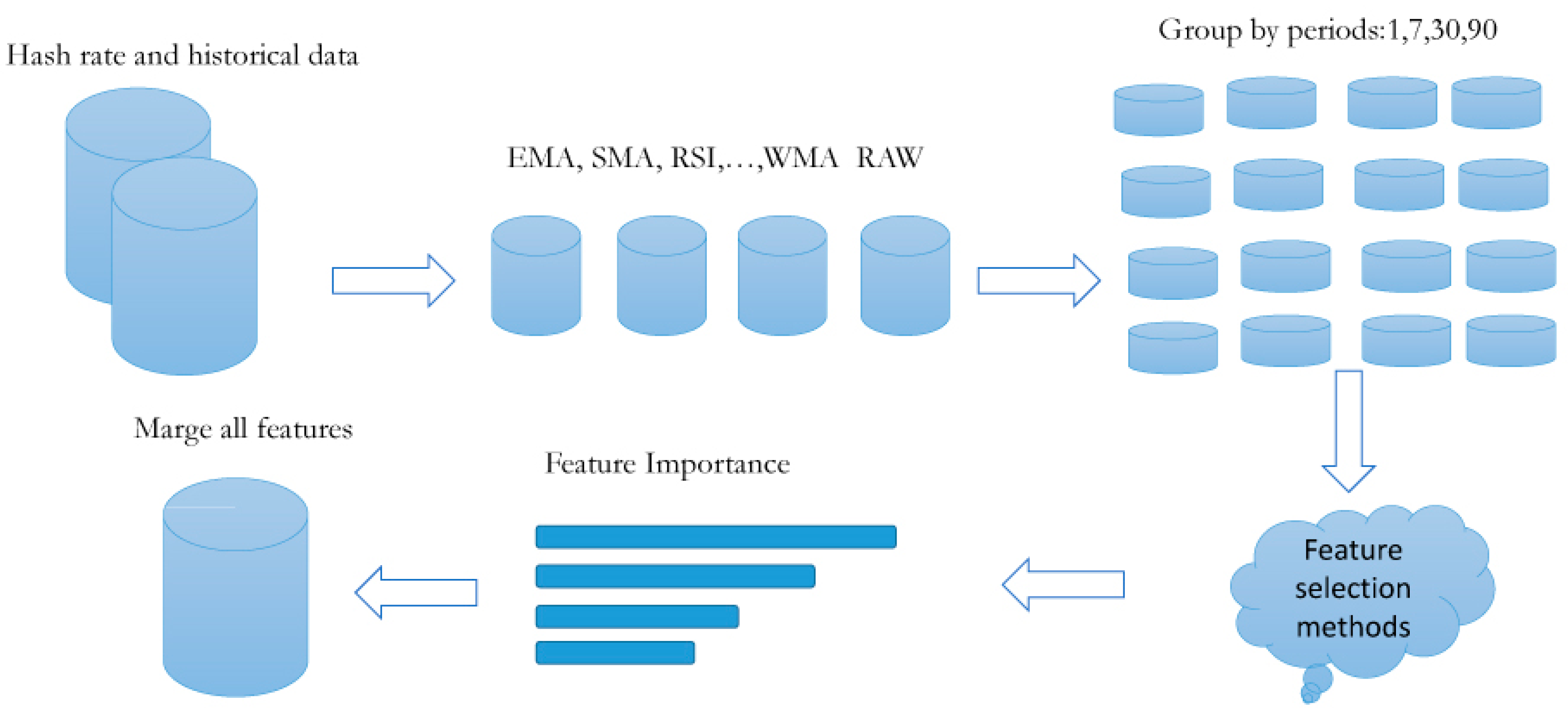
This section will discuss the data collection, preprocessing, feature selection, and how to prepare labels. Therefore, this section includes the subsequent three subsections. An overview of the data collection and manipulation process is shown in Figure 1.

Figure 1. Data collection and manipulation flowchart.

4.1. Hash Rate Data Collection (Feature Vector)

At first, the Bitcoin dataset, which includes Bitcoin hash rate information, was collected. Bitcoin features and price data are available online for free. The data of this study was collected from https://bitinfocharts.com (accessed on 18 September 2023) using a web scraper written in Python 3.6. More than 700 features were collected based on technical indicators. We used the same process as in [45] for the data collection. The feature selection method selected a smaller subset of features from this large set of features. Technical indicators including simple moving average (SMA), exponential moving average (EMA), relative strength index (RSI), weighted moving average (WMA), standard deviation (STD), variance (VAR), triple exponential moving average (TRIX), and rate of change (ROC) were used for these data. According to the preprocessing performed in [45], the missing value cases were quantified using the linear interpolation method as much as possible. For all regression and classification models, the dataset was shuffled and divided into two sets: the training set and validation set. A total of 20% of the data were kept for validation, and 80% of the data were used for training. On the other hand, the isolation forest method algorithm [46] was used to control outliers. This algorithm removed approximately 14% of the outlier data. Next, the features selected for each interval are listed in Table 2.

4.2. Computational Linguistics Data Collection (Linguistic Vector)

This section extracts some of the most important features to recognize effective tweets. These features are known as linguistic features:

• Numbers of words and sentences: The number of words in tweets is distributed in a broad spectrum, which shows that some fake tweets have very few words and some have many words. Word count is just a simple view for analyzing tweets. In addition, actual tweets have more sentences on average than fake tweets. These features are considered under ${WS}_{count}$, which is a 2D vector (including the average number of tweets) per day.
• Question marks, exclamation marks, and capital letters: Considering the text of the tweets, it can be concluded that spam tweets have more punctuation marks than actual tweets. Real tweets have fewer question marks than spam tweets. The reason may be that there are many rhetorical questions in spam tweets. These rhetorical questions are always used to emphasize ideas and intensify emotions consciously. This 3-dimensional vector is called the ${QEC}_{count}$ vector (includes the average number of tweets per day).
• Psychological perspective: From a psychological perspective, we also examine using first person pronouns (e.g., I, we, and me) in real and fake tweets. Deceptive people often use language that minimizes self-reference. A person who lies tends not to use “we” and “I” and does not use personal pronouns. On average, fake tweets have fewer first-person pronouns. We define the vector extracted from this step as P h, which contains the average number of daily tweets.
• Sentiment analysis: TextBlob (https://textblob.readthedocs.io/en/dev/ (accessed on 18 September 2023)) library was used for sentiment analysis. TextBlob is a Python (2 and 3) library for processing textual data. It is a simple API used in common natural language processing (NLP) tasks such as part-of-speech tagging, noun phrase extraction, sentiment analysis, classification, translation, and more. This library from NLTK (Natural Language ToolKit) uses the main core, and the input contains a single sentence, while the outputs of the TextBlob are the polarity and subjectivity. The polar score ranges from (−1 to 1), where −1 indicates the most negative words, such as “disgusting”, “awful”, and “pathetic”, and 1 indicates the most positive words such as “excellent” and “best”. It specifies if the subjectivity score is between (0 to 1), which shows the number of personal opinions. If a sentence has a high subjectivity, i.e., close to 1, it seems the text contains more personal opinions than real information. We call the vector extracted from this step a binary, Se, which contains the average number of tweets per day.

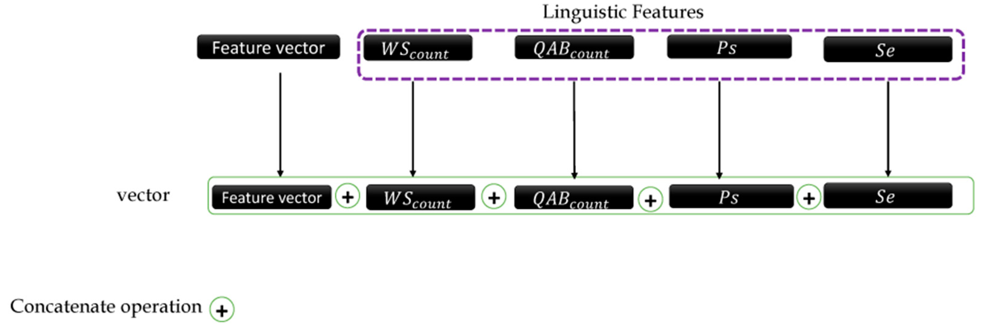
The combination of different extracted features is shown in Figure 2.

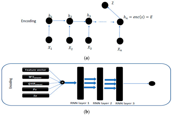
Figure 2. (a) Chart proposed for the encoding phase. (b) Architecture of the proposed approach for illiquidity prediction.

The outline of the proposed approach is shown in Figure 3, where the encoding layer is placed with RNN layers, which are discussed in the following three types of layers that are placed:

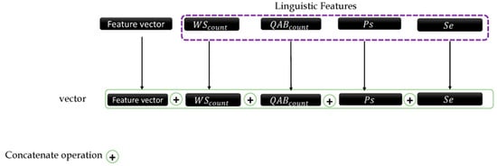
Figure 3. Linguistic features flowchart.

4.3. Illiquidity Label

In [47], they considered a new method for measuring illiquidity, which is the basis of summarizing the data of this research. Assuming that w, d, h, and m represent the weekly, daily, hourly, and minute intervals, the interval of each of these values is equal to w = [1; :::; W], d = [1; 2; :::; 7], h = [00; 01; :::; 23], and m = [00; 01; :::; 59], and W refers to the weekly interval in data collection. According to the research in [38], to measure volatility and volume patterns, we introduce the relative measures of volatility and volume in days, hours, and minutes. For this purpose, we measure volatility using the absolute return instead of the squared return. The reason is that absolute returns are less sensitive than flat regions and are sufficient to measure relative volatility. Complete efficiency and its closely associated amplitude-based measures constitute common metrics for gauging and modeling volatility. The use of absolute returns holds an advantage, as they, coupled with volume, contribute to the computation of the illiquidity measures outlined below. Relative measures exhibit heightened robustness, especially when linked to mean variables confined within the range of zero to one.

$${\lambda }_{\sigma }^{day}(d)\equiv \frac{1}{N_d}\sum _w\frac{7{\sum }_{h.m}\left|y_{\tau }(w,d,h,m)\right|}{{\sum }_{i=0}^6{\sum }_{h,m}^{}\left|y_{\tau }(w,d-i,h,m)\right|}$$

(20)

and

$${\lambda }_v^{day}(d)\equiv \frac{1}{N_d}\sum _w\frac{7{\sum }_{h.m}\left|V_{\tau }(w,d,h,m)\right|}{{\sum }_{i=0}^6{\sum }_{h,m}^{}\left|V_{\tau }(w,d-i,h,m)\right|}$$

(21)

Here, $N_d\simeq W$ is the number of observations on day d in the measurement sample ${(N}_d=Wor{N}_d=W-1)$. If we consider the example with d = 1 (Mondays), ${\lambda }_{\sigma }^{day}\left(d\right)$ and ${\lambda }_V^{day}\left(d\right)$ measure the volatility and volume that occurs on Mondays relative to other days of the week, respectively.

Also, $\lambda$ = 1 corresponds to the average level of volatility and volume, respectively. Similarly, the relative measures of volatility and volume for the hour of the day are given by the following equations:

$${\lambda }_{\sigma }^{hour}(h)\equiv \frac{1}{N_h}\sum _{w,d}\frac{24{\sum }_m\left|y_{\tau }(w,d,h,m)\right|}{{\sum }_{i=0}^{23}{\sum }_m\left|y_{\tau }(w,d-i,h,m)\right|}$$

(22)

and

$${\lambda }_V^{hour}(h)\equiv \frac{1}{N_h}\sum _{w,d}\frac{24{\sum }_m\left|V_{\tau }(w,d,h,m)\right|}{{\sum }_{i=0}^{23}{\sum }_m\left|V_{\tau }(w,d-i,h,m)\right|}$$

(23)

For h = 0, …, 23 and the number of observations h indicated by $N_h$, we will have the value of $N_h\simeq 7\ast W$. The authors in [47] combined their volatility and volume measures into a relative liquidity measure based on Amihud’s method [32]. First, they calculated the liquidity measure for each hour and compared the hourly measure with the average of the previous 24 h. The measurement of their relative illiquidity was defined as follows:

This illiquidity calculation method was used for the target dataset.

The data at three main intervals are given in Table 3 as it was gathered. In this table, the amount of training and test data are given.

$${\lambda }_{illiquid}^{hour}(h)\equiv \frac{1}{N_d}\frac{Illiq(w,d,h)}{{\sum }_{j=0}23IIIiq(w,d,h-i)}$$

(24)

where

$$Illiq\left(w,d,h\right)\equiv \frac{{\sum }_m\left|y_{\tau }(w,d,h,m)\right|}{v_{\tau }(w,d,h)}$$

(25)

Table 3. Intervals of data and training and test size.

Dataset	Interval 1	Interval 2	Interval 3
Range	April 2013–July 2016	April 2013–April 2017	April 2013–April 2022
# Records	1206	1462	3285
# Train (80%)	964	1169	2628
# Test (20%)	242	293	657

5. Results

In this section, the impact of each of the feature sets that was introduced in the data collection section is explained to show the impact of these features on Bitcoin illiquidity prediction and to determine issues that can be improved. A description of each of the models and their inputs is given below, and a summary of the symbols used in the models is provided in Table 4.

Table 4. Parameter spaces for each parameter name.

Parameter Name	Dimension	Features
Feature vector	$R^{20}$	Median_transaction_fee30 trx USD
		Median transaction fee 7 trx USD
		Price 90 emaUSD
		Size 90 trx
		Transactions
		Price 30 wma USD
		Price 3 wma USD
		Price 7 wma USD
		Median transaction fee 7 roc USD
		Difficulty 30 rsi
		Mining profitability
		Price 30 sma USD
		Sentinusd 90 ema USD
		Transaction value USD
		Top 100 cap
		Difficulty 90 mom
		Hashrate 90 var
		Price 90 wma USD
		Sent in usd 90 sma USD
		Median transaction tee USD
${Ws}_{count}$	$R^2$	Word count and sentence count
${QEC}_{count}$	$R^3$	Question mark, exclamation mark and capital letters count
Ph	$R^1$	Physiology
SE	$R^2$	Polarity and subjectivity

Several different models were proposed to examine this analysis, which we will discuss in the following section:

• RNN (feature vector and ${Ws}_{count}$): The input of this model is all the extracted indicator features and the features related to the number of words and sentences of tweets on that day. In fact, the feature space of this model is equal to $R^{20}$ + $R^2$.
• RNN (feature vector and ${QEC}_{count}$): The input of this model is all the extracted indicator features and the features related to the number of question marks, exclamation marks, and capital letter counts of tweets on that day. In fact, the feature space of this model is equal to $R^{20}$ + $R^3$.
• RNN (feature vector and Ph): In this model, the features of the feature vector and Ph are used as input features. The feature space of this model is equal to $R^{20}$ + $R^1$.
• RNN (feature vector and SE): In this model, the features of the feature vector and Ph are used as input features. The feature space of this model is equal to $R^{20}$ + $R^2$.
• RNN (all features): This model incorporates all features as inputs, encompassing the entire feature space of previously considered cases and combinations, denoted as $R^{20}$ + $R^2$ + $R^3$ + $R^1$ + $R^2$.

Various evaluation methods were employed to assess the models, as outlined below, with both split validation and cross-validation applied to address the predictive problem:

• Split validation: This method involves dividing the dataset into training and test groups, with the training set typically larger than the test set. The training dataset is utilized for training a machine learning model, while the test dataset evaluates the trained model. Both datasets feature a label attribute containing the prediction column indicating the degree of illiquidity.
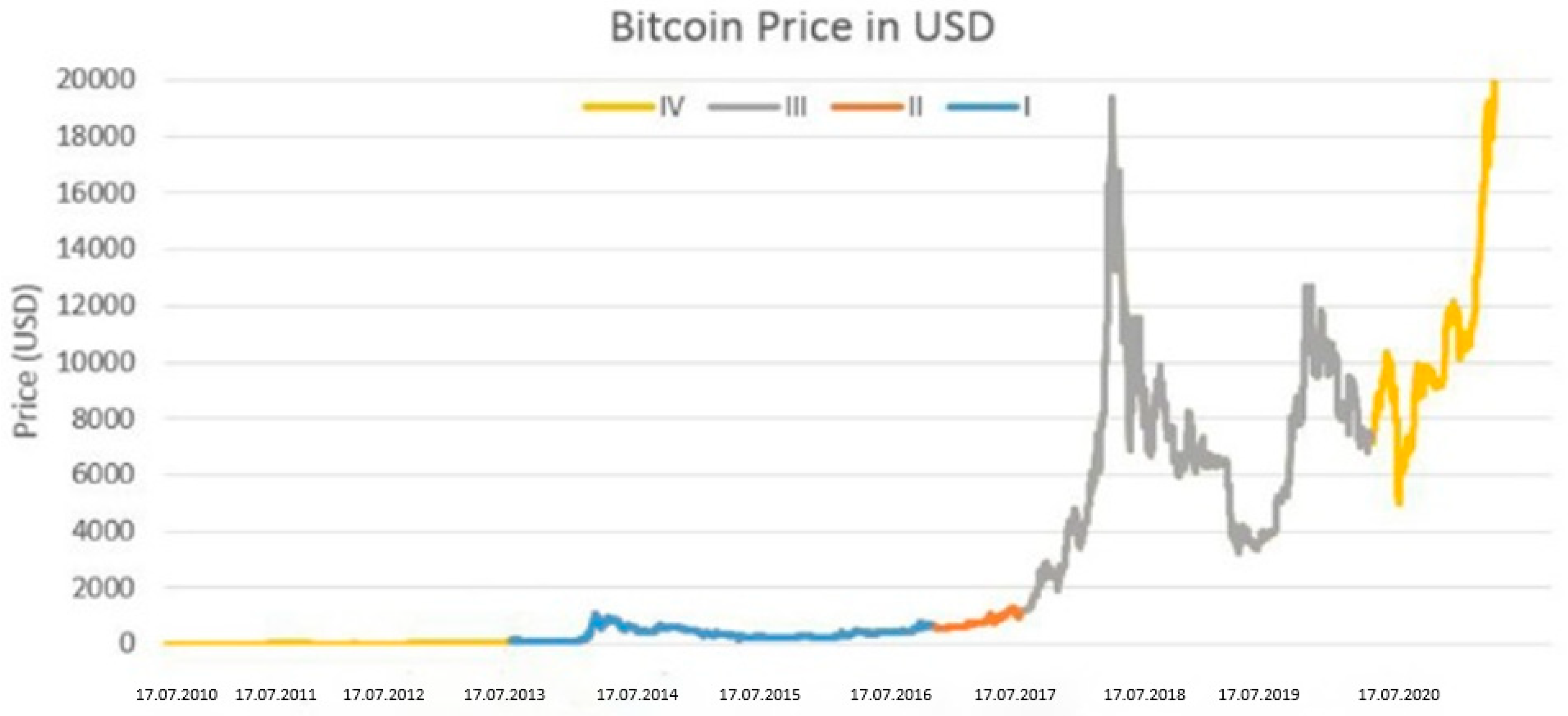
• Cross-validation: In this method, the dataset is partitioned into N groups, with each group serving as the test set in the turn, while the remaining groups are used for training. The ultimate outcome is the average of the results obtained from each group. Although cross-validation is recognized as more demanding, it typically produces more dependable results. However, caution is advised in this study when predicting the early illiquidity of Bitcoin based on its prior price, as this is the focus of cross-validation. Examining Figure 4, the Bitcoin price chart illustrates a significant historical price surge, accompanied by increased volatility in recent years. Forecasting the price in the initial years incurs less error due to this substantial rise. Given that these early years outnumber the preceding years with the highest prices, the average forecast error for this period is considerably lower. Averaging the errors across all cross-validation groups mitigates the impact of inaccurate forecasting in later years, resulting in the lowest error occurring in the initial years and a substantial reduction in the final mean error. This phenomenon gives the illusion of effective prediction for the machine learning algorithm. Consequently, split validation is considered more reliable for predicting Bitcoin’s illiquidity, prioritizing the anticipation of the cryptocurrency’s future trajectory over its initial prices.
  

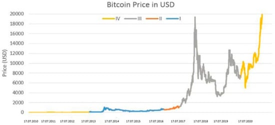  Figure 4. Bitcoin price chart.

Both methods use a sampling method to divide the initial dataset. There are also two well-known sampling methods as follows:

• Linear: This approach preserves the order of the records based on the original dataset. For example, suppose the split ratio is 80% and 20% for the training and testing datasets. In that case, the training dataset will be the first 80% of the initial dataset, and the test dataset will be the last 20%.
• Random: This strategy involves the random selection of unique records from the original dataset, while ensuring the distribution ratio of label features is maintained in both the training and testing datasets.

However, the drawback of the random approach becomes apparent when selecting records from Bitcoin data from the last year and earlier, which may introduce bias when predicting the future of the digital currency. Anticipating the illiquidity of Bitcoin becomes more manageable when armed with knowledge about its illiquidity on specific days of the last month. Hence, a preference is given to employing a linear approach for cryptocurrency forecasting.

Unfortunately, the plain paper did not consider these facts and used cross-validation in some experiments and split validation in others. Because of their differences, as discussed, their results are different. Additionally, it uses a random approach to sampling, which, as discussed, is again unfair. However, the article fortunately publishes its code base with its dataset.

Therefore, we modify and implement its code for the linear partitioning validation approach. Also, the article considered the basis of its proposed approaches for price prediction, which we considered for illiquidity, which is comparative primarily.

First, in Table 5, the results of the proposed RNN approaches and the approaches used in [36] are shown to predict the price of Bitcoin. These approaches are as follows:

Table 5. Baseline paper results for different validation methods for (all features).

Validation Method ↓	Metrics →	MAE ($)			MAPE (%)
	Intervals → Model ↓	I	II	III	I	II	III
Random split (paper)	ANN	0.45	2.61	9.50	1.08	1.28	2.78
	SVM	0.72	3.23	7.04	0.74	1.28	1.44
	SANN	0.24	2.13	4.58	0.55	0.93	2.73
	LSTM	0.20	4.55	6.90	0.95	1.95	3.61
	Simple RNN	0.67	3.2	3.67	0.72	1.21	1.42
	GRU	0.22	2.12	3.23	0.56	1.19	1.51
	IndRNN	0.21	1.99	3.89	0.45	0.93	1.04
Random split (run)	ANN	1.05	8.12	6.37	3.00	8.22	1.32
	SVM	1.23	5.37	9.47	0.96	2.09	2.21
	SANN	1.06	5.77	7.45	2.96	6.13	1.22
	LSTM	0.55	4.47	5.54	0.68	1.70	1.11
	Simple RNN	1.22	2.41	9.40	0.98	2.53	2.01
	GRU	1.45	3.65	6.66	0.69	1.91	1.12
	IndRNN	0.52	1.21	5.01	0.65	1.83	1.19
Linear split (run)	ANN	8.21	9.4	8.50	5.70	22.2	3.21
	SVM	2.04	6.19	9.87	0.87	14.49	7.51
	SANN	2.75	12.7	12.13	3.89	9.58	2.10
	LSTM	2.83	5.02	14.77	3.75	1.18	2.51
	Simple RNN	2.05	6.12	6.10	0.90	1.51	7.92
	GRU	2.40	5.67	4.87	3.80	1.90	3.01
	IndRNN	2.01	4.80	3.89	3.70	1.15	2.42

• Artificial neural network (ANN): The neural network considered in the study is characterized by specific hyperparameters: optimizer (Adam), hidden layers with neurons (2 layers with 128 neurons each), learning rate (0.08), epoch (5000), batch size (64), activation function (ReLU), and loss function (logcosh). The original article discusses the application of this network in both regression and classification modes. However, for our purposes, we specifically employed the regression mode to predict illiquidity.
• Stacked artificial neural network (SANN): In this approach, five ANN networks were considered with the settings mentioned in the ANN approach. A SANN consists of five individual ANNs that are used to train a larger ANN model. Individual models are trained using training data with a fivefold cross-validation; each model is trained with the same configuration in a separate layer. Since ANNs have random initial weights, each trained ANN gets different weights, and this advantage enables them to learn their differences well. This network is used in two modes of regression and classification in the basic article, and we used the regression mode to predict illiquidity.
• Support vector machines (SVM): This algorithm is a supervised ML model that operates based on the idea of separating points using a hyperplane, and in fact, its primary goal is to maximize the margin. In SVM, kernels can be linear or nonlinear depending on the data and include the radial basis function (RBF), hyperbolic tangent, and polynomial kernels. This algorithm can provide predictions with a low error rate for small datasets without much training. In the introductory article, this approach is considered with the Gaussian RBF kernel, which was considered only in its regression mode to predict the illiquidity of this approach.
• Long short-term memory: This approach is an RNN network that uses four gates to learn long sequences. In the previous section, RNN approaches were discussed. This approach is used in both regression and classification modes, and in this research, its regression mode was used depending on the types of labels.

To gauge the effectiveness of the regression models, their performance is evaluated using key metrics: the mean absolute error (MAE), root mean square error (RMSE), and mean absolute percentage error (MAPE). A favorable model is characterized by minimizing the MAE, MAPE, and RMSE values.

$$\mathrm{M}\mathrm{A}\mathrm{E}=\frac{1}{n}\sum _{i=1}^n\left|y_i-{\widehat{y}}_i\right|$$

(26)

$$\mathrm{R}\mathrm{M}\mathrm{S}\mathrm{E}=\sqrt{\frac{1}{n}\sum _{i=1}^n{\left|y_i-{\widehat{y}}_i\right|}^2}$$

(27)

$$\mathrm{M}\mathrm{A}\mathrm{P}\mathrm{E}=\frac{100}{n}\sum _{i=1}^n\frac{\left|y_i-{\widehat{y}}_i\right|}{y_i}$$

(28)

Keras stands out as a Python-based high-level library that seamlessly adapts to both GPU and CPU settings. Offering a diverse set of modules encompassing neural layers, cost functions, optimizers, initialization schemes, activation functions, and regularization, this API played a pivotal role in realizing artificial neural networks (ANN), sparse artificial neural networks (SANN), long short-term memory networks (LSTM), and recurrent neural networks (RNNs). In the case of support vector machines (SVM), the implementation drew upon the capabilities of the SKlearn library.

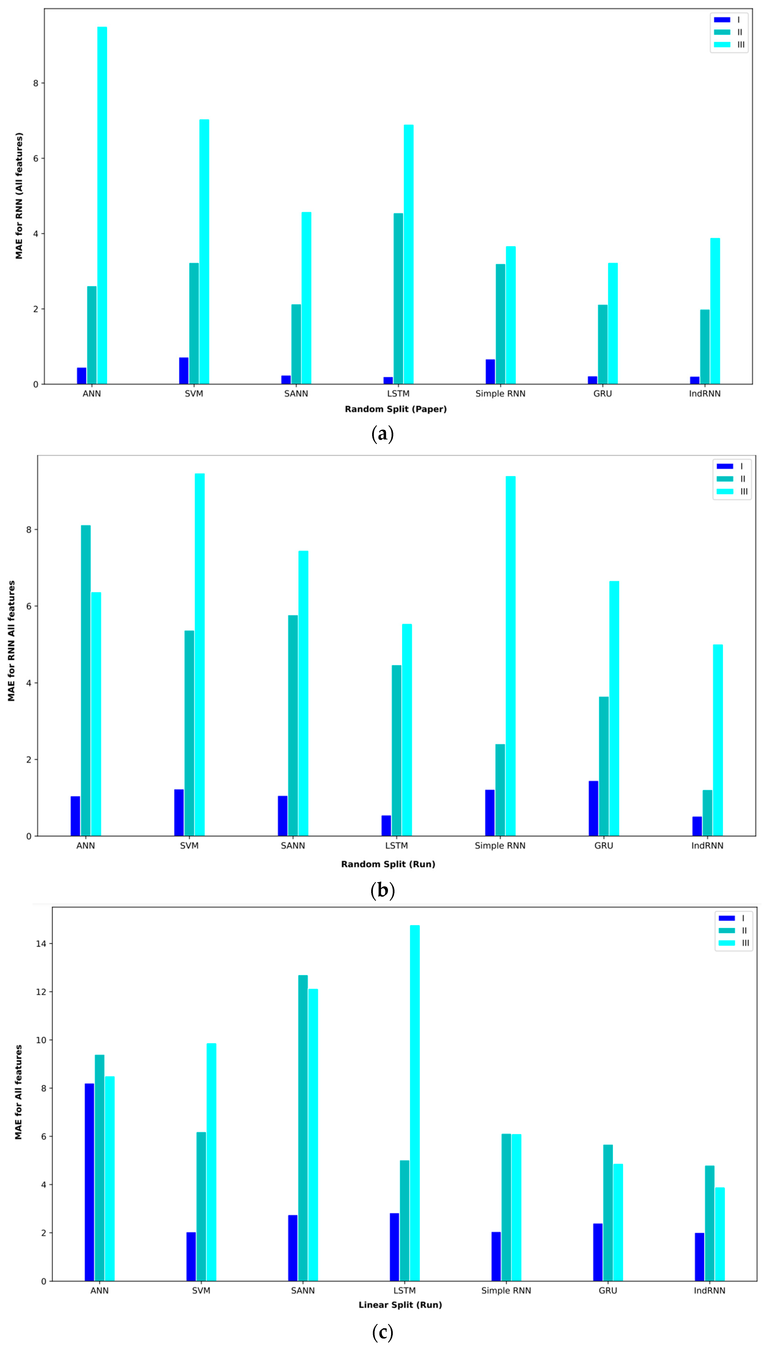
The results of the regression models for three intervals in the mode of using all the features are given in Table 5. In the first period, from April 2013 to July 2016, BTC prices did not experience much volatility, and hence, the illiquidity level was also low. In this interval, all the models have performed the predictions well. In random split (paper) mode, the proposed IndRNN approach obtained an MAE = 0.21, the most favorable MAE value. On the other hand, this approach reached a MAPE = 0.45, the lowest value in the reported results. In the random split (run) evaluation model, the IndRNN approach again obtained the most favorable results in terms of the MAE and MAPE. This approach achieved an MAE = 0.52 and a MAPE = 0.65 in the interval I. The linear split (run) gave poorer results than the random split (paper) and random split (run). In this evaluation method, the IndRNN could reach an MAE = 2.01 and a MAPE = 3.70, which are the most favorable results.

In interval II, from April 2013 to April 2017, BTC prices are significantly higher than at the end. However, it is relatively more stable compared to interval I. This interval has a significant amount of illiquidity due to price fluctuations. In the random split (paper) evaluation method, the IndRNN approach recorded an MAE = 1.99, which is the lowest MAE among other approaches. However, the IndRNN and SANN approaches performed equally in the MAPE criterion and achieved a MAPE = 0.93. In random split (run), the IndRNN approach reached an MAE = 1.21, and the LSTM approach reached a MAPE = 1.7, the most favorable results in the reported results. The linear split (run) still recorded weaker results in this interval and reached an MAE = 4.80 for IndRNN and a MAPE = 1.18 for LSTM in the most favorable mode. The LSTM approach recorded acceptable results in terms of the MAPE in this interval.

The Bitcoin price experienced the highest volatility since April 2017, which was covered in interval III (April 2013 to December 2019). In parallel, the lack of liquidity in this interval is more than in the other intervals. In the random split (paper) evaluation method, the GRU approach achieved an MAE = 3.23, and the IndRNN approach reached a MAPE = 1.04 in this interval, which are the best results among the tested approaches. In random split (run), the IndRNN approach reached an MAE = 5.01, and the GRU approach reached a MAPE = 1.12, which were the most favorable results. In this performance evaluation method, the two GRU and IndRNN approaches were the opposite of the random split (paper) method regarding the MAE and MAPE. Also, in linear split (run), the IndRNN approach achieved the best result, reaching an MAE = 3.98 and a MAPE = 2.42.

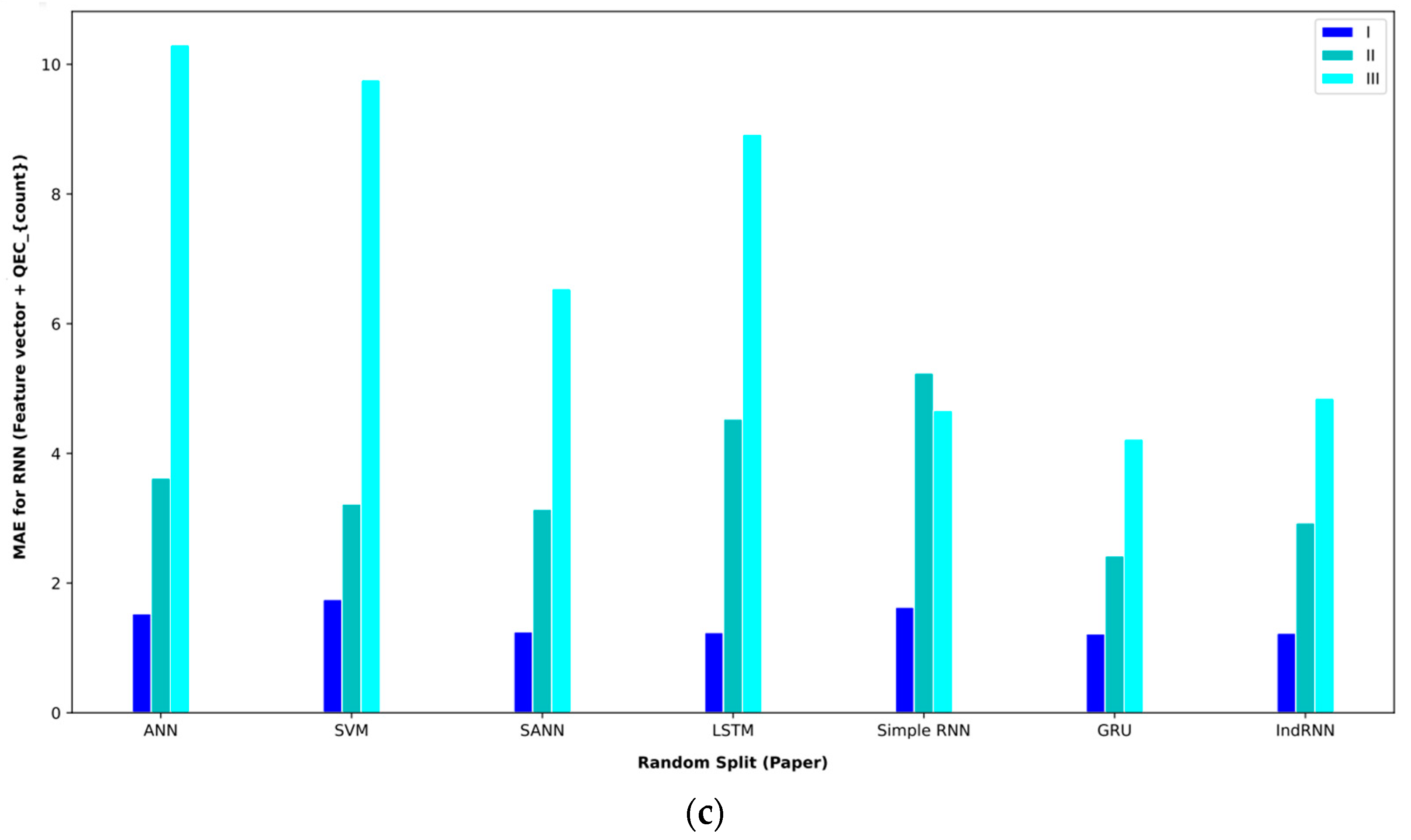
Next, Table 6 shows the results of the proposed approaches and other approaches on the feature vector $and{QEC}_{count}$. In comparing the different approaches on interval I, the GRU approach obtained the best result and achieved an MAE = 1.22.

Table 6. p-values of difference approaches.

Model	ANN	SVM	SANN	LSTM	Simple RNN	GRU	IndRNN
ANN	Statistic = 0.0, p-value = 1.0, df = 34.0	Statistic = −0.0622, p-value = 0.9507, df = 34.0	Statistic = −0.17560, p-value = 0.8616, df = 34.0	Statistic = −0.0071, p-value = 0.9943, df = 34.0	Statistic = −0.3070, p-value = 0.76069, df = 34.0	Statistic = −0.1642, p-value = 0.8704, df = 34.0	Statistic = −0.2393, p-value = 0.8122, df = 34.0
SVM	Statistic = 0.0622, p-value = 0.9507, df = 34.0	Statistic = 0.0, p-value = 1.0, df = 34.0	Statistic = −0.1134, p-value = 0.9103, df = 34.0	Statistic = 0.0551, p-value = 0.9563, df = 34.0	Statistic = −0.2453, p-value = 0.8076, df = 34.0	Statistic = −0.1020, p-value = 0.9192, df = 34.0	Statistic = −0.1773, p-value = 0.8602, df = 34.0
SANN	Statistic = 0.1756, p-value = 0.8616, df = 34.0	Statistic = 0.1134, p-value = 0.9103, df = 34.0	Statistic = 0.0, p-value = 1.0, df = 34.0	Statistic = 0.168, p-value = 0.8671, df = 34.0	Statistic = −0.1323, p-value = 0.8954, df = 34.0	Statistic = 0.0115, p-value = 0.9908, df = 34.0	Statistic = −0.0640, p-value = 0.9493, df = 34.0
LSTM	Statistic = 0.0071, p-value = 0.9943, df = 34.0	Statistic = −0.0551, p-value = 0.9563, df = 34.0	Statistic = −0.1685, p-value = 0.8671, df = 34.0	Statistic = 0.0, p-value = 1.0, df = 34.0	Statistic = −0.2999, p-value = 0.7660, df = 34.0	Statistic = −0.1571, p-value = 0.8760, df = 34.0	Statistic = −0.2322, p-value = 0.8177, df = 34.0
Simple RNN	Statistic = 0.3070, p-value = 0.7606, df = 34.0	Statistic = 0.2453, p-value = 0.8076, df = 34.0	Statistic = 0.1323, p-value = 0.8954, df = 34.0	Statistic = 0.2999, p-value = 0.76606, df = 34.0	Statistic = 0.0, p-value = 1.0, df = 34.0	Statistic = 0.1439, p-value = 0.8863, df = 34.0	Statistic = 0.06848, p-value = 0.9457, df = 34.0
GRU	Statistic = 0.1642, p-value = 0.8704, df = 34.0	Statistic = 0.1020, p-value = 0.9192, df = 34.0	Statistic = −0.01152, p-value = 0.9908, df = 34.0	Statistic = 0.1571, p-value = 0.8760, df = 34.0	Statistic = −0.14391, p-value = 0.8863, df = 34.0	Statistic = 0.0, p-value = 1.0, df = 34.0	Statistic = −0.0755, p-value = 0.9401, df = 34.0
IndRNN	Statistic = 0.2393, p-value = 0.8122, df = 34.0	Statistic = 0.1773, p-value = 0.8602, df = 34.0	Statistic = 0.0640, p-value = 0.9493, df = 34.0	Statistic = 0.2322, p-value = 0.8177, df = 34.0	Statistic = −0.0684, p-value = 0.9457, df = 34.0	Statistic = 0.0755, p-value = 0.9401, df = 34.0	Statistic = 0.0, p-value = 1.0, df = 34.0

This result was obtained using the random split (paper) policy (Table 7). The indRNN approach was the second, and the LSTM approach was the third-best approach in this interval. In examining the approaches on interval II, the IndRNN approach can obtain a better MAE. This approach obtained an MAE = 2.08 in interval 2, which was obtained using the random split (run) evaluation method. Also, in this interval, the second-best model is GRU. In examining interval III, the IndRNN approach again obtained the lowest MAE. This approach has performed worse in the MAPE comparison than the LSTM-based approach. In the validation method, according to the obtained results, the random split (paper) approach obtained the best result on average, and the linear split (run) approach obtained the worst result.

Table 7. Baseline paper results for different validation methods for (feature vector and QEC_counter).

Validation Method ↓	Metrics →	MAE ($)			MAPE(%)
	Intervals → Model ↓	I	II	III	I	II	III
Random split (paper)	ANN	1.53	3.62	10.3	2.98	2.38	4.35
	SVM	1.75	3.22	9.76	1.70	2.77	2.43
	SANN	1.25	3.14	6.54	1.56	1.89	5.55
	LSTM	1.24	4.53	8.92	1.94	2.09	2.13
	Simple RNN	1.63	5.24	4.66	1.76	1.64	2.42
	GRU	1.22	2.42	4.22	1.54	1.16	2.78
	IndRNN	1.23	2.93	4.85	1.08	1.95	2.15
Random split (run)	ANN	2.53	4.63	8.39	4.31	9.24	3.64
	SVM	2.33	9.63	11.5	1.89	4.13	3.15
	SANN	2.83	6.75	8.49	3.94	7.89	2.54
	LSTM	1.75	5.91	6.57	1.38	2.13	2.25
	Simple RNN	2.23	2.98	10.42	1.31	2.19	3.19
	GRU	2.44	6.63	8.64	1.13	2.12	2.08
	IndRNN	1.47	2.08	7.91	0.98	2.85	2.42
Linear split (run)	ANN	9.46	10.24	9.93	4.78	25.3	4.42
	SVM	3.34	8.08	10.83	1.47	16.41	9.04
	SANN	3.73	13.91	13.10	4.22	11.12	3.24
	LSTM	3.33	6.93	15.74	4.34	3.17	3.54
	Simple RNN	3.35	7.13	7.12	1.43	3.13	7.90
	GRU	3.65	7.09	5.24	5.52	3.92	4.24
	IndRNN	2.23	5.78	4.06	5.72	3.88	2.98

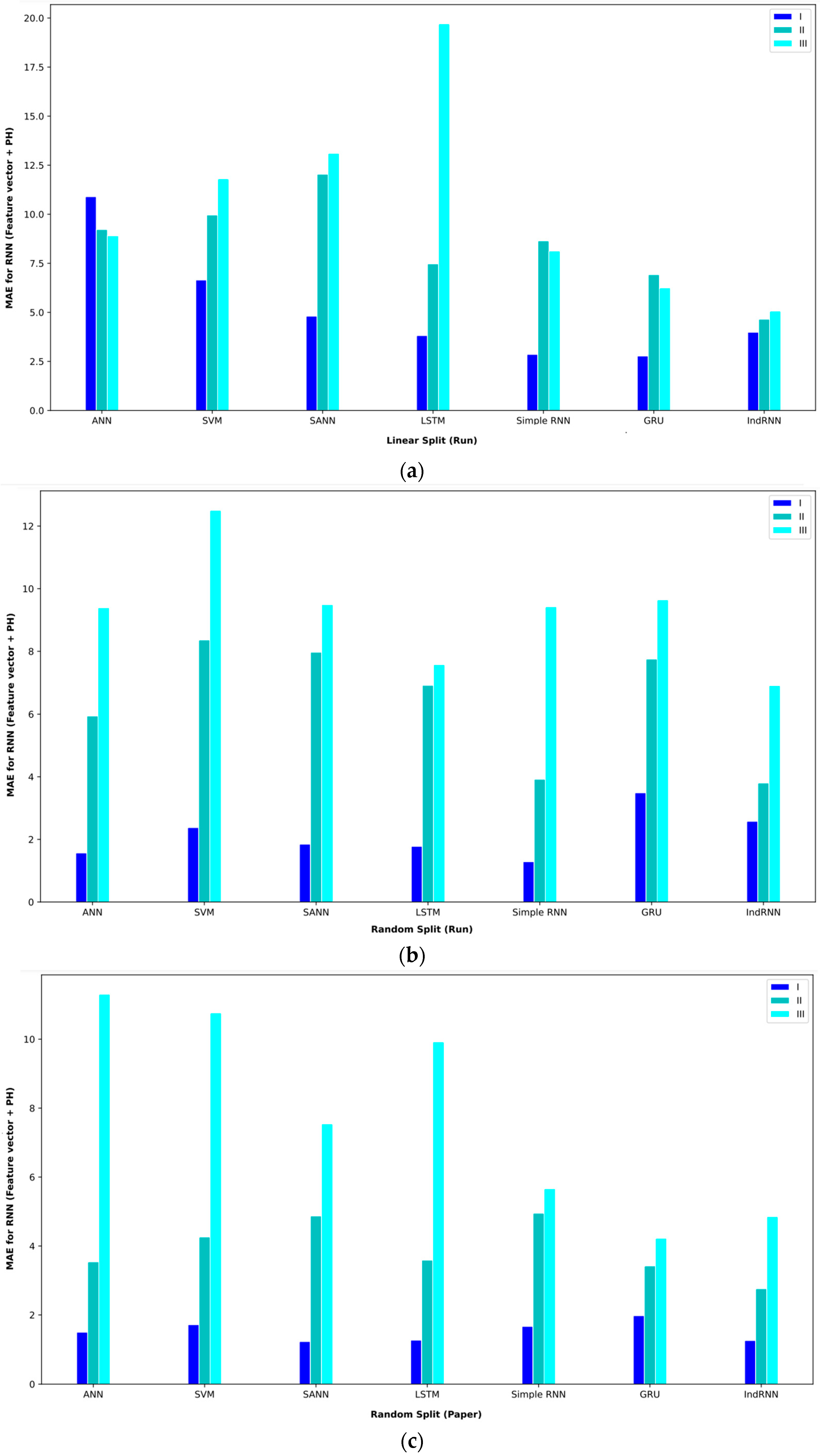
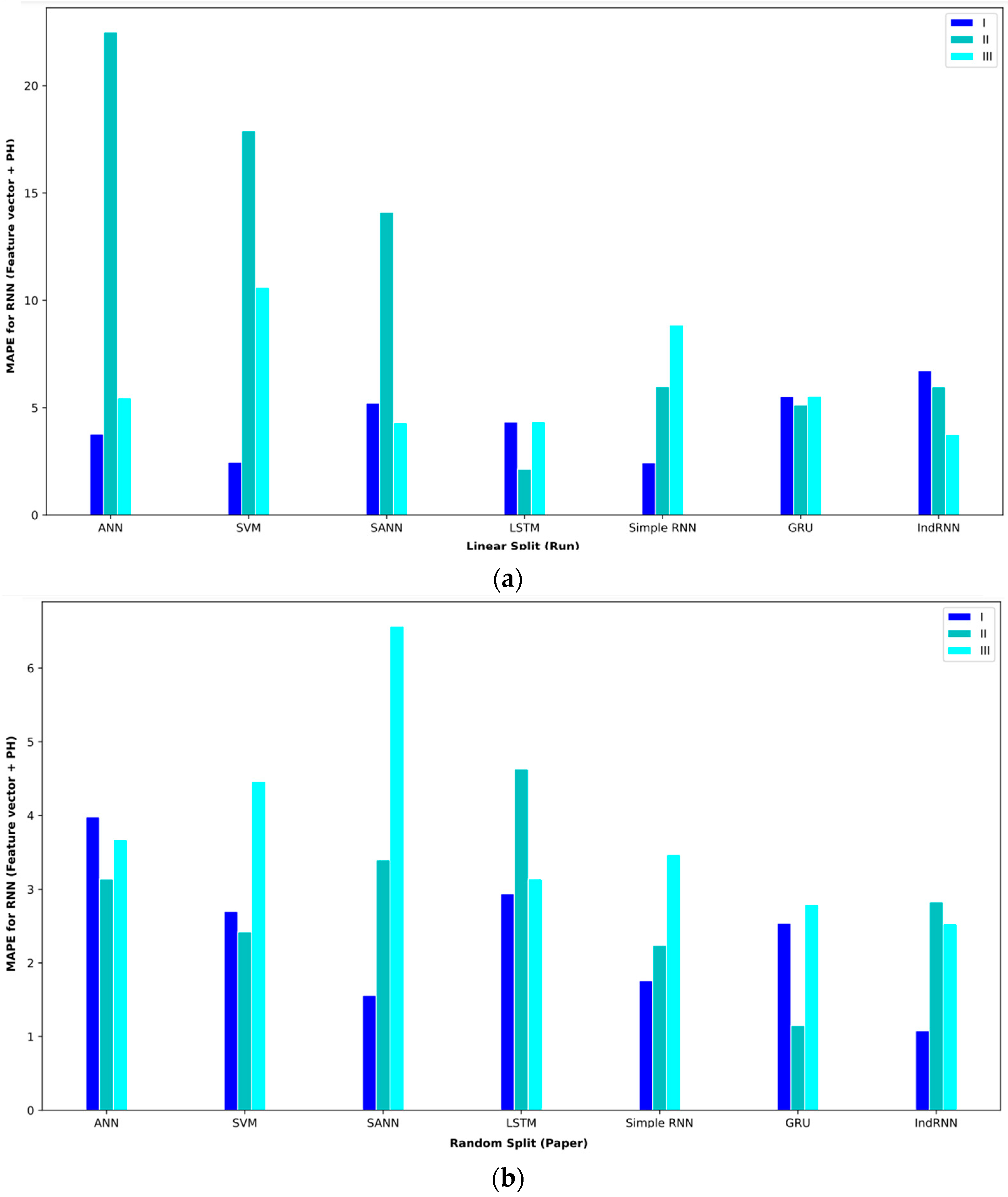
Table 8 shows the results of different approaches for the feature vector and Ph. In interval I, the SANN approach with a validation method based on random split (paper) could reach an MAE = 1.23. The second-best approach in this interval was the IndRNN approach, which achieved an MAE = 1.26. In interval II, RNN-based approaches performed better; the IndRNN approach reached an MAE = 2.76 and the GRU approach reached an MAE = 3.42, which were the first- and second-best models in this interval, respectively. These results were obtained using the validation method based on random split (paper). In interval III, the GRU approach performed better than other approaches and achieved an MAE = 4.22 with the validation method based on random split (paper).

Table 8. Baseline paper results for different validation methods for (feature vector and Ph).

Validation Method ↓	Metrics →	MAE ($)			MAPE (%)
	Intervals → Model ↓	I	II	III	I	II	III
Random split (paper)	ANN	1.50	3.54	11.3	3.98	3.14	3.67
	SVM	1.72	4.26	10.76	2.70	2.42	4.46
	SANN	1.23	4.87	7.54	1.56	3.40	6.57
	LSTM	1.27	3.59	9.92	2.94	4.63	3.14
	Simple RNN	1.67	4.95	5.66	1.76	2.24	3.47
	GRU	1.98	3.42	4.22	2.54	1.15	2.79
	IndRNN	1.26	2.76	4.85	1.08	2.83	2.53
Random split (run)	ANN	1.57	5.94	9.39	5.31	5.13	5.67
	SVM	2.38	8.36	12.5	2.89	6.38	2.24
	SANN	1.85	7.97	9.49	4.94	4.14	4.75
	LSTM	1.78	6.92	7.57	1.38	4.13	4.23
	Simple RNN	1.29	3.92	9.42	3.31	2.30	2.65
	GRU	3.49	7.75	9.64	2.13	2.17	3.61
	IndRNN	2.58	3.80	6.91	1.98	2.43	3.42
Linear split (run)	ANN	10.98	9.22	8.93	3.78	22.5	5.46
	SVM	6.65	9.96	11.83	2.47	17.93	10.6
	SANN	4.81	12.04	13.10	5.22	14.14	4.29
	LSTM	3.82	7.47	19.74	4.34	2.14	4.34
	Simple RNN	2.86	8.64	8.12	2.43	5.98	8.85
	GRU	2.78	6.92	6.24	5.52	5.13	5.53
	IndRNN	3.99	4.65	5.06	6.72	5.97	3.75

Combining extracted features and SE features in the feature vector and SE also obtained comparable results. Table 9 shows the results of these features and proposed approaches. In interval I, the GRU approach obtained the best result. This approach with the validation method based on random split (paper) reached an MAE = 0.53. In this routine, the second-best approaches were the simple RNN and LSTM, which achieved an MAE = 1.23. In interval II, the IndRNN approach with a validation method based on random split (paper) could reach an MAE = 1.55 and the GRU approach reached an MAE = 5.22 in interval III, which are, respectively, the best approaches in intervals II and III.

Table 9. Baseline paper results for different validation methods for the feature vector and SE.

Validation Method ↓	Metrics →	MAE ($)			MAPE (%)
	Intervals → Model ↓	I	II	III	I	II	III
Random split (paper)	ANN	2.51	2.56	10.3	4.98	3.14	3.67
	SVM	2.31	5.56	11.7	3.70	2.42	4.46
	SANN	1.25	5.25	6.54	2.56	3.40	6.57
	LSTM	1.23	5.54	10.92	1.94	4.63	3.14
	Simple RNN	1.23	3.42	6.66	2.72	1.24	4.47
	GRU	0.53	2.23	5.22	1.12	2.15	4.79
	IndRNN	1.55	1.55	5.85	4.81	3.83	5.53
Random split (run)	ANN	2.23	5.42	10.39	4.32	6.13	2.67
	SVM	2.3	8.14	11.5	1.29	5.38	3.24
	SANN	1.89	7.91	10.49	5.93	3.14	3.75
	LSTM	2.24	6.24	7.57	2.12	5.13	3.23
	Simple RNN	1.23	3.54	9.42	3.32	2.30	2.65
	GRU	2.43	8.23	9.64	2.31	4.17	4.61
	IndRNN	1.12	4.82	5.91	1.32	7.43	5.42
Linear split (run)	ANN	13.40	8.25	8.93	5.13	23.5	6.46
	SVM	7.24	8.23	10.83	2.43	13.93	9.6
	SANN	5.24	10.3	13.10	5.23	15.14	5.29
	LSTM	4.98	8.23	14.74	4.54	4.14	5.34
	Simple RNN	1.68	8.52	5.12	2.09	3.98	7.85
	GRU	4.42	6.23	7.24	5.89	4.13	3.53
	IndRNN	3.24	5.42	6.06	4.33	6.97	4.75

The analysis of features based on the statistics of sentences and words is also given in Table 10. In interval I, the GRU approach obtained the lowest MAE = 1.14. Meanwhile, the ANN approach was able to get the second-best result. Both approaches in random split (paper) obtained these results. In interval II, the ANN approach in random split (paper) achieved an MAE = 1.56, the best performance. In interval III, the IndRNN approach in random split (run) achieved an MAE = 6.91, which had better results than other approaches.

Table 10. Baseline paper results for different validation methods for (feature vector and ${Ws}_{count}$).

Validation Method ↓	Metrics →	MAE ($)			MAPE (%)
	Intervals → Model ↓	I	II	III	I	II	III
Random split (paper)	ANN	1.53	1.56	12.3	3.08	2.14	3.67
	SVM	2.34	6.56	13.7	2.24	3.42	4.46
	SANN	2.22	6.25	6.54	1.34	4.40	6.57
	LSTM	2.25	3.54	11.92	2.93	5.63	3.14
	Simple RNN	2.15	5.42	7.66	2.43	3.66	3.40
	GRU	1.14	2.23	6.22	3.76	2.35	2.73
	IndRNN	2.13	2.55	7.85	2.04	2.64	2.24
Random split (run)	ANN	3.21	4.42	11.39	4.34	5.42	6.43
	SVM	3.32	2.14	16.5	1.43	6.42	2.65
	SANN	3.81	4.91	11.49	5.93	4.10	4.35
	LSTM	2.21	2.24	8.57	2.36	4.15	4.09
	Simple RNN	2.22	5.54	10.42	1.35	2.34	2.24
	GRU	2.43	9.23	10.64	1.13	2.90	3.66
	IndRNN	2.11	3.82	6.91	2.94	2.65	3.46
Linear split (run)	ANN	11.2	10.9	9.93	2.73	22.6	5.35
	SVM	8.23	10.3	11.83	3.48	17.2	10.8
	SANN	6.22	11.3	11.10	4.25	14.9	4.34
	LSTM	5.94	13.0	16.74	5.36	2.90	4.30
	Simple RNN	3.61	12.5	6.12	3.44	5.23	8.42
	GRU	2.42	11.0	8.24	5.53	5.42	5.65
	IndRNN	3.23	11.0	7.06	6.71	5.23	3.74

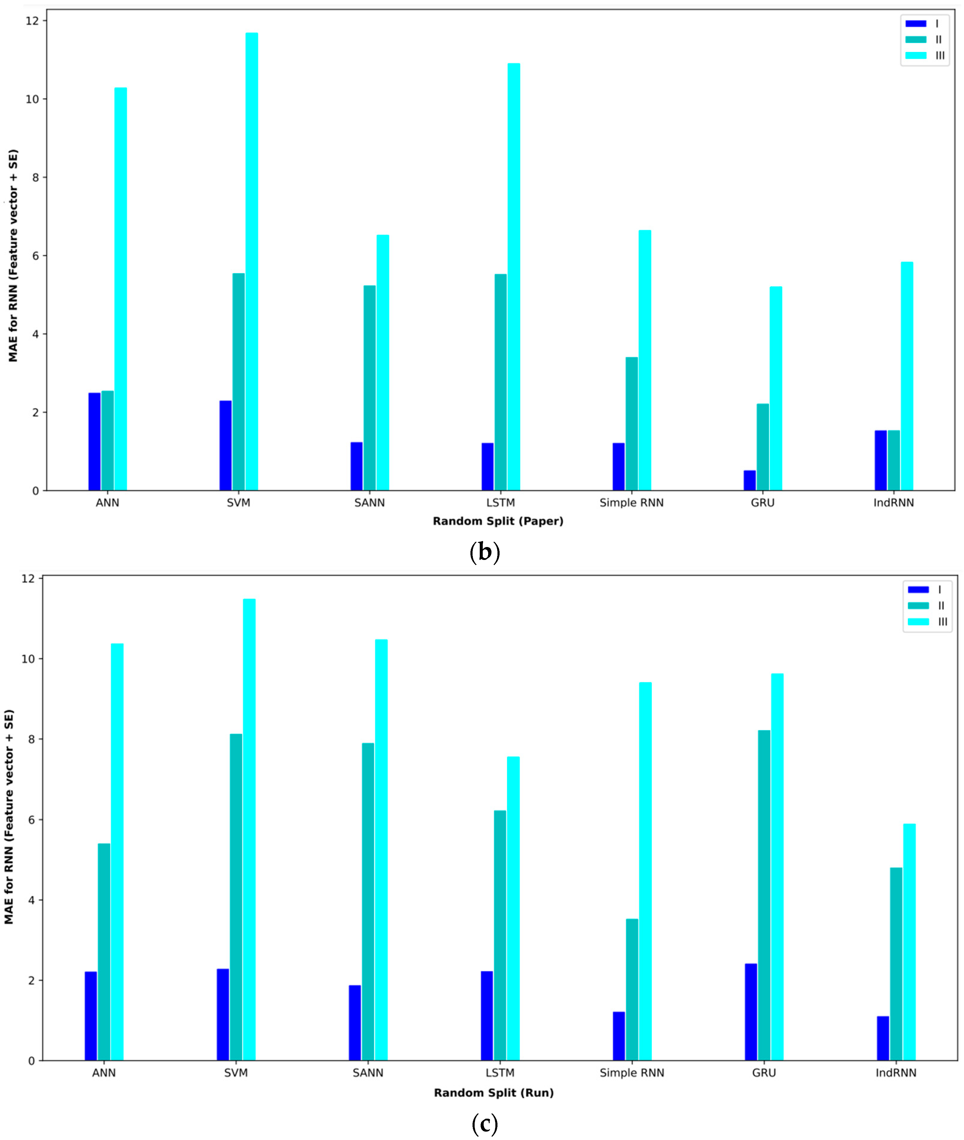
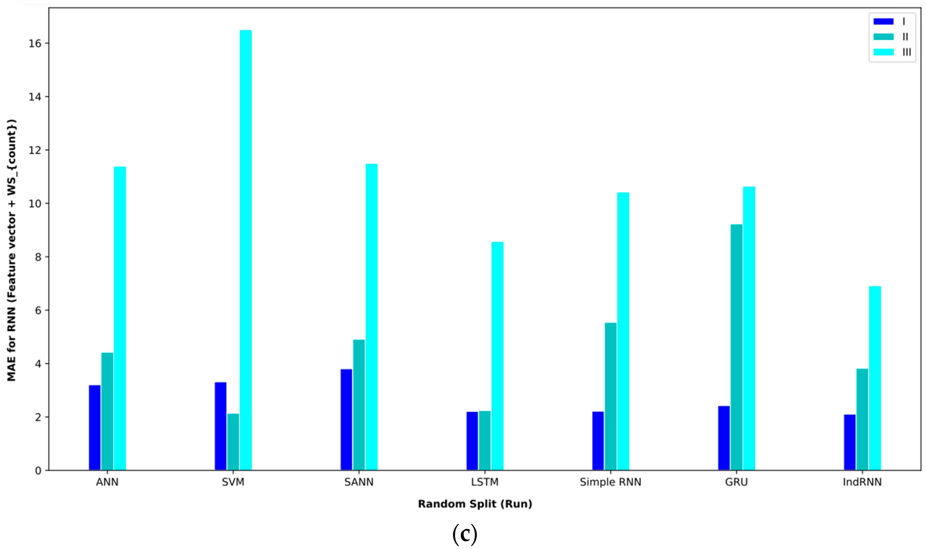
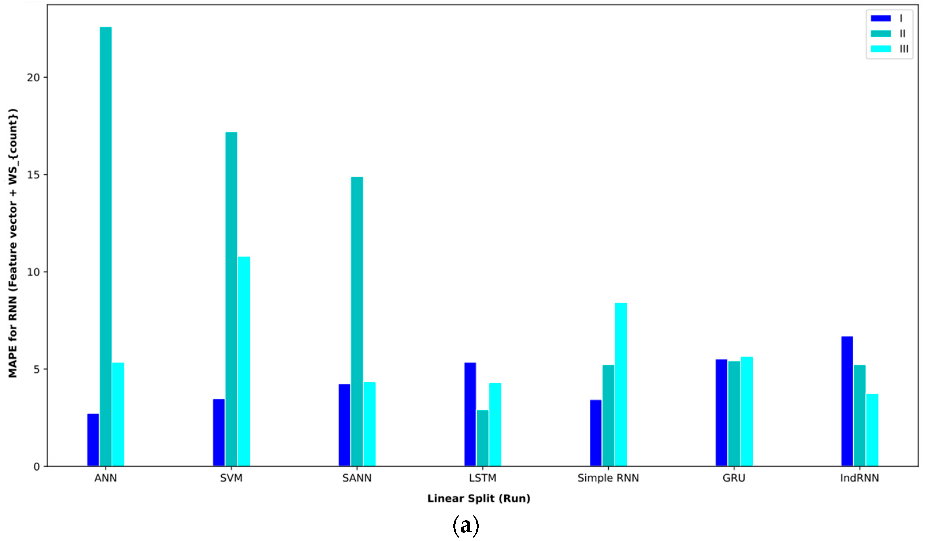
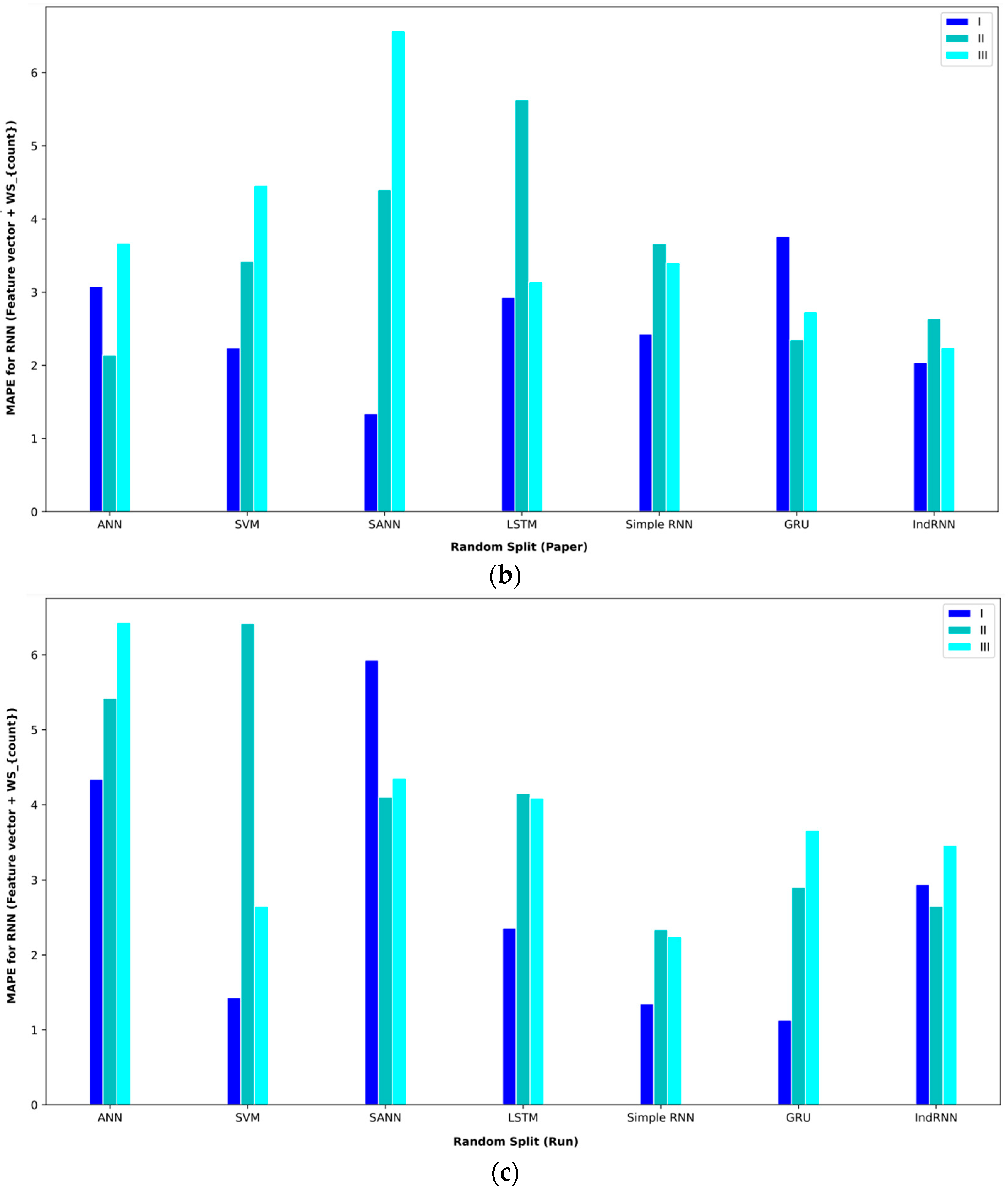
In order to better display the proposed approaches, bar plot charts of different criteria are shown in Figure 5, Figure 6, Figure 7, Figure 8, Figure 9, Figure 10, Figure 11, Figure 12, Figure 13 and Figure 14.

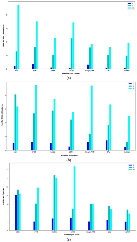
Figure 5. Bar plot of MAEs for different approaches where all features are considered input to the models.

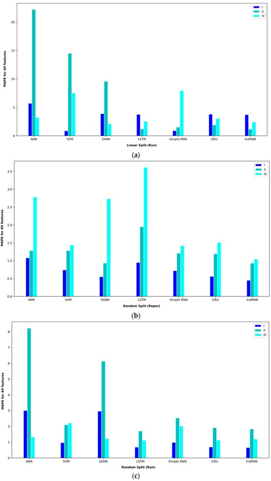
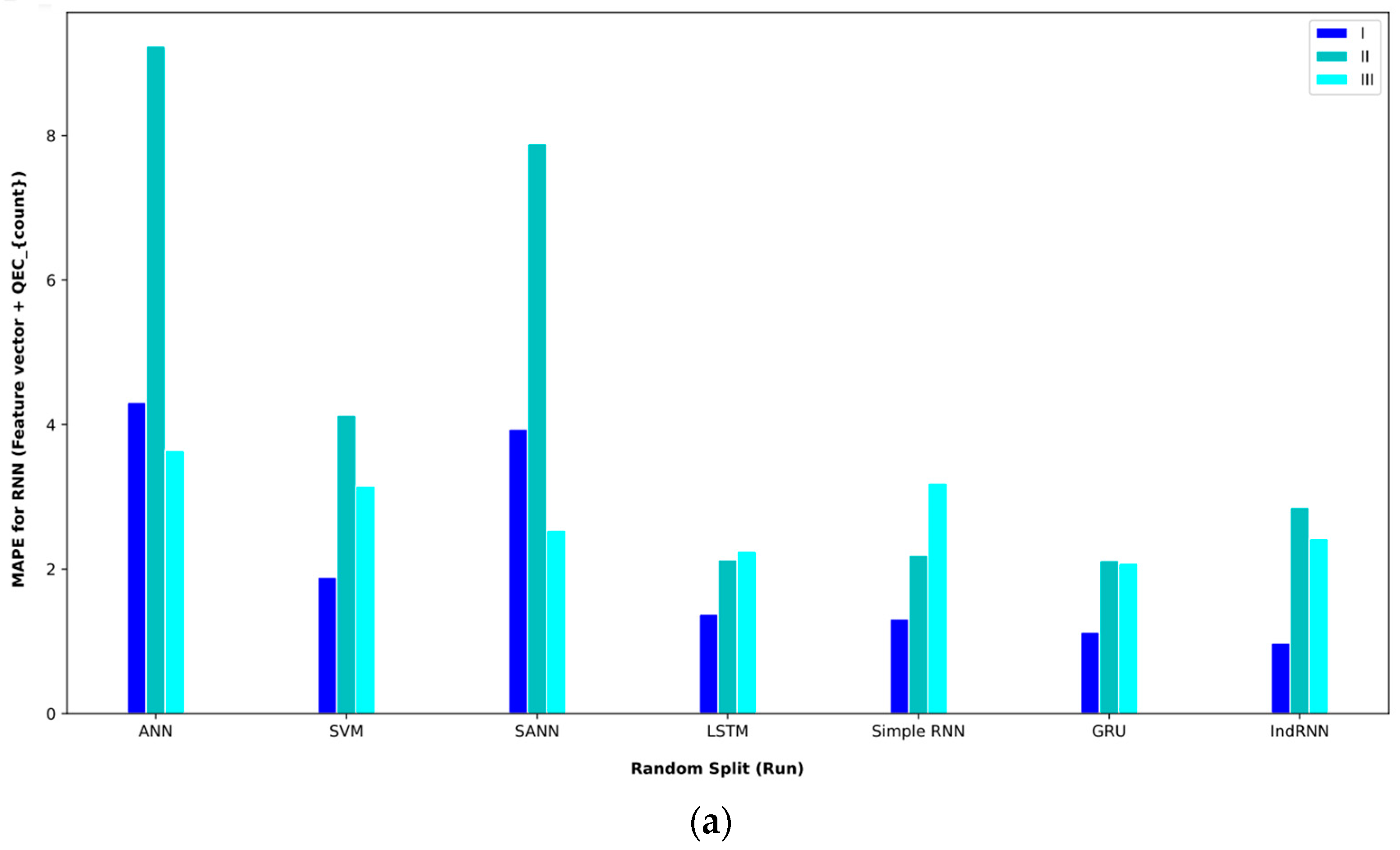
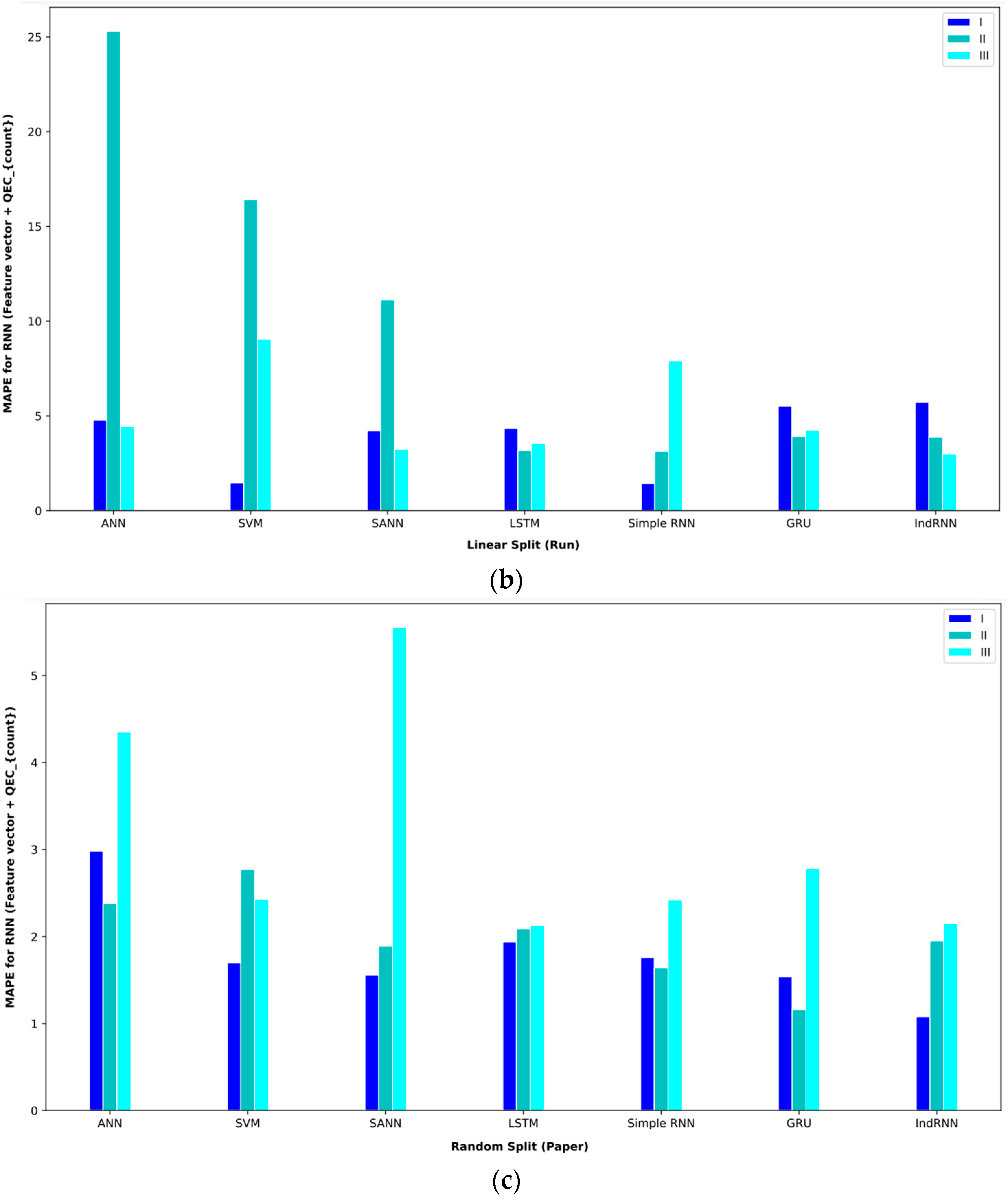
Figure 6. Bar plot of MAPEs for different approaches where all features are considered input to the models.

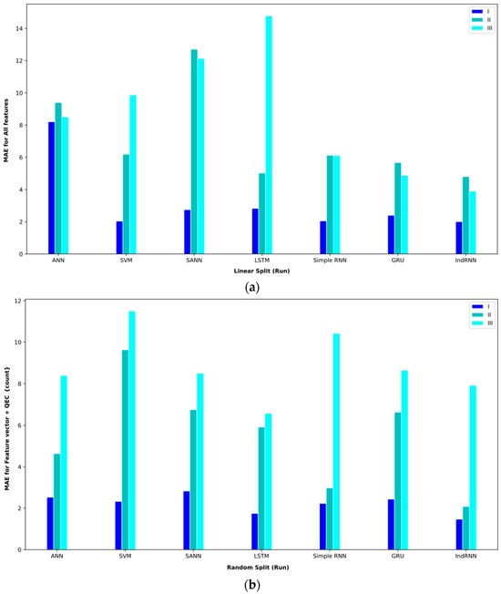
Figure 7. Bar plot of MAEs for different approaches where the feature vector and ${QEC}_{count}$ are considered input to the models.

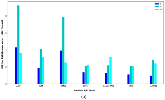
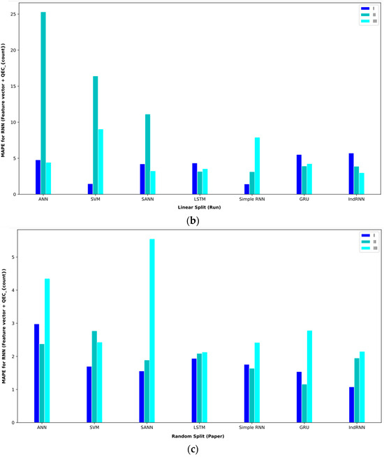
Figure 8. Bar plot of MAPEs for different approaches where the feature vector and ${QEC}_{count}$ are considered input to the models.

Figure 9. Bar plot of MAEs for different approaches where the feature vector and Ph are considered input to the models.

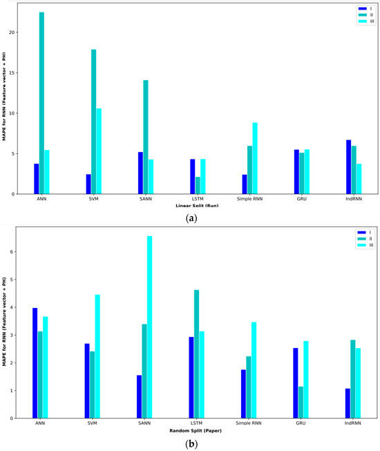
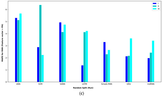
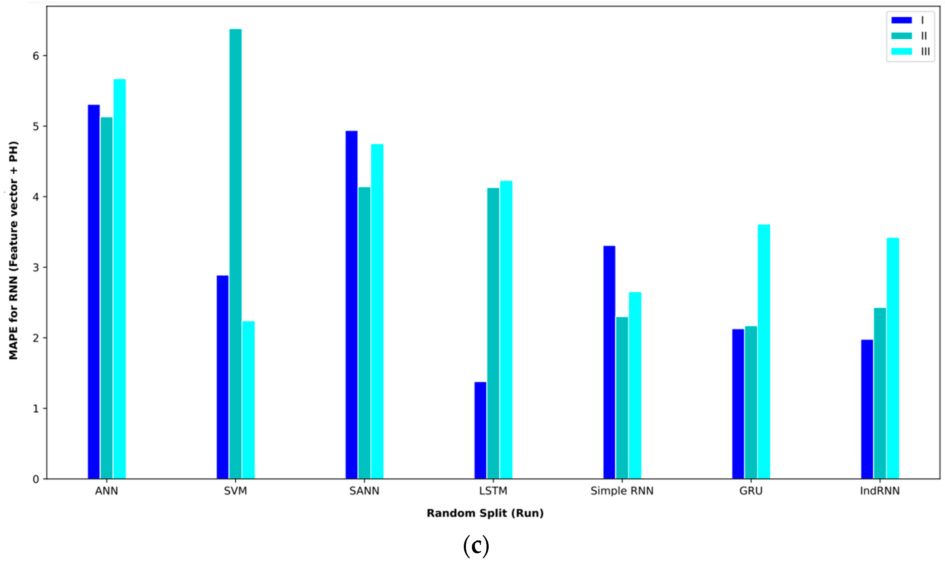
Figure 10. Bar plot of MAPEs for different approaches where the feature vector and Ph are considered input to the models.

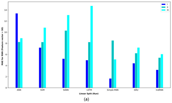
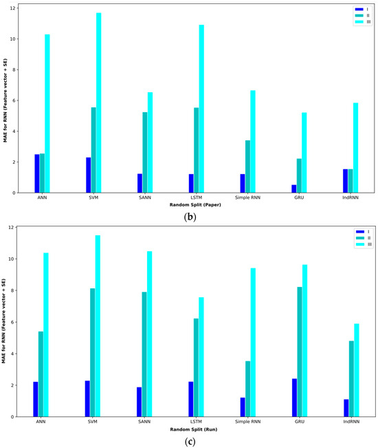
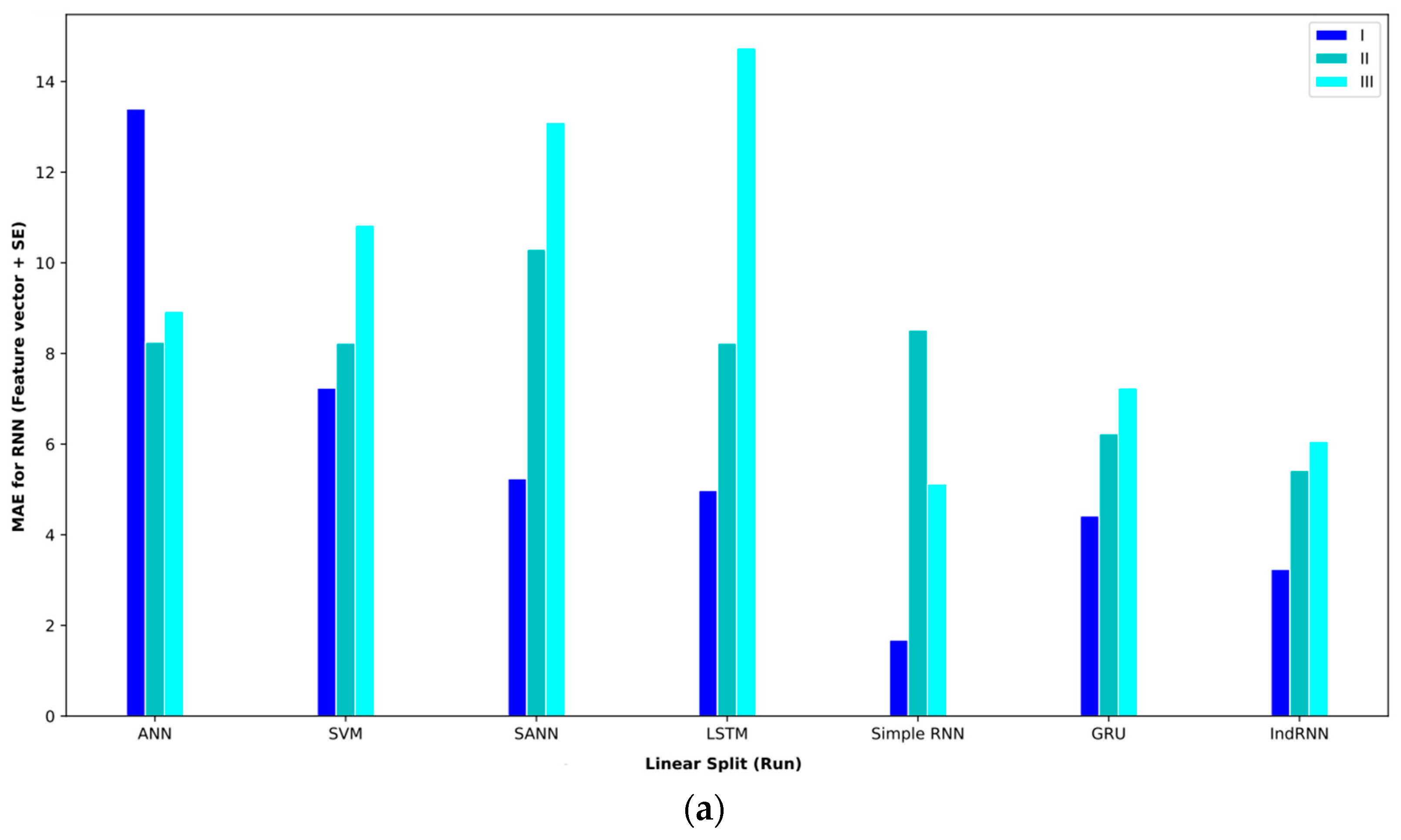
Figure 11. Bar plot of MAEs for different approaches where the feature vector and SE are considered input to the models.

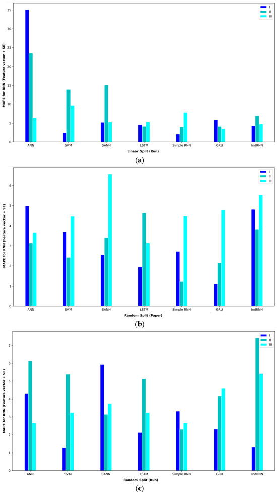
Figure 12. Bar plot of MAPEs for different approaches where the feature vector and SE are considered input to the models.

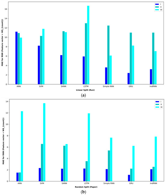
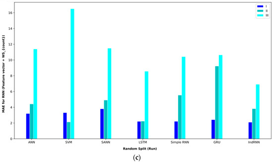
Figure 13. Bar plot of MAEs for different approaches where the feature vector and ${Ws}_{count}$ are considered input to the models.

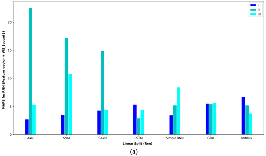
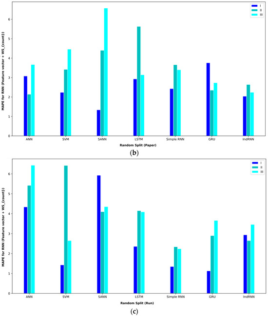
Figure 14. Bar plot of MAPEs for different approaches where the feature vector and ${Ws}_{count}$ are considered input to the models.

In order to check the research hypotheses, the p-values of different approaches are given in Table 6.

6. Conclusions and Gap Analysis

This research aimed to predict short-term and medium-term Bitcoin market illiquidity using time series models and machine learning algorithms. We found that the IndRNN algorithm is a better predictor than other approaches due to the nonlinearity of market liquidity and the complexity of its market microstructure. Considering a time series analysis, the IndRNN model performs better for capturing short-term liquidity, while the LSTM and GRU models also provide acceptable results. Despite the above results, limitations in this study can be seen. First, the sample used in this study is small; the data history used in this research is considered in the daily interval, which reduces the number of training samples. Secondly, base cryptocurrencies and altcoins have much less history than Bitcoin, which makes it challenging to present a model for them.

The research on digital currency liquidity and its prediction through machine learning approaches holds several potential implications for management. These implications encompass risk management, portfolio optimization, data splitting policies, market stability, investor confidence, strategic decision making, adoption of hybrid forecasting approaches, regulatory compliance, and the incorporation of advanced technologies. Decision makers can leverage the findings to proactively manage the risks associated with digital currency investments, enhance portfolio efficiency, adopt effective data splitting strategies, attract investors through improved market liquidity, inform strategic decisions using predictive models, comply with evolving regulatory frameworks, and explore the adoption of advanced technologies for enhanced financial analysis. In essence, the research offers valuable insights that can guide managerial actions and strategies in navigating the complexities of digital currency markets.

In the realm of future research, there lies an opportunity to delve into alternative GARCH-type models, paving the way for a comprehensive comparative analysis. A model of interest in this exploration is the VAR-BEKK-GARCH model, as put forth by Loverta and López [33], specifically tailored for the analysis of time series data concerning log spreads. Nevertheless, a significant hurdle to overcome in this endeavor is the infrequent occurrence of certain intervals. A potential solution to this challenge involves the categorization of these intervals into distinct classes. Depending on the representation of minority classes, strategies for controlling minority class influence can be applied, presenting an avenue to fortify the robustness of the analytical approach. This problem is an unbalanced sampling problem for which the following approaches can be used:

• Resampling: Time series forecasting is a challenging task where the nonstationary characteristics of the data require strict settings for forecasting tasks.

A common problem is the skewed distribution of the target variable, where some intervals are highly significant but severely underrepresented. Standard regression tools focus on the average behavior of the data. However, the goal in many time series forecasting tasks is the opposite.

For example, predicting rare values is one of these challenges. A standard solution for time series forecasting with unbalanced data is to use resampling strategies that operate on the learning data by changing their distribution in favor of a particular bias. Various algorithms have been proposed for this purpose. For example, algorithms in Ref. [41] can be used.

• High-dimensional imbalanced time-series classification (OHIT) [42]: OHIT first uses a density ratio-based joint nearest-neighbor clustering algorithm to capture minority class states in a high-dimensional space.

Depending on different clustering algorithms, this clustering can get different results. It then for each mode applies the shrinkage technique of a large-dimensional covariance matrix to obtain an accurate and reliable covariance structure. Finally, OHIT generates structure-preserving synthetic samples based on a multivariate Gaussian distribution using the estimated covariance matrices.

• IB-GAN [48]: The standard methods of class weight, oversampling, or data augmentation are the approaches studied in “An empirical survey of data augmentation for time series classification with neural networks”.

These approaches are parametric. Parametric approaches do not always yield significant improvements for predicting the minority classes of interest. Nonparametric data augmentation with generative adversarial networks (GANs) is a promising solution.

For this purpose, the authors have proposed the imputation balanced GAN (IBGAN), which combines a new method of augmentation and data classification in a one-step process through an imputation balance approach. An IB-GAN uses imputation and resampling techniques to generate higher-quality samples from randomly masked vectors than white noise, and balances the classifier through a pool of real and synthetic samples. Hyperparameter imputation pmiss allows us to regularize the classifier variation by adjusting the innovations introduced through generator imputation. The IB-GAN is simple to train and model, pairing each deep learning classifier with a generator discriminator pair, resulting in higher accuracy for less observed classes. The basis of this approach is a GAN that tries to generate cases similar to the minority class.

The authors in [49] showed the effect of different features for stock forecasting, and in other future works, these ideas can be used for illiquidity prediction.

References

- Huberman, G.; Leshno, J.; Moallemi, C.C. An economic analysis of the bitcoin payment system. Columbia Bus. Sch. Res. Pap. 2019, 17, 92. [Google Scholar]
- Sensoy, A. The inefficiency of Bitcoin revisited: A high-frequency analysis with alternative currencies. Financ. Res. Lett. 2019, 28, 68–73. [Google Scholar] [CrossRef]
- Saito, T. Bitcoin: A Search-Theoretic Approach. In Digital Currency: Breakthroughs in Research and Practice; IGI Global: Hershey, PA, USA, 2019; pp. 1–23. [Google Scholar]
- Mensi, W.; Al-Yahyaee, K.H.; Kang, S.H. Structural breaks and double long memory of cryptocurrency prices: A comparative analysis from Bitcoin and Ethereum. Financ. Res. Lett. 2019, 29, 222–230. [Google Scholar] [CrossRef]
- Kajtazi, A.; Moro, A. The role of bitcoin in well diversified portfolios: A comparative global study. Int. Rev. Financ. Anal. 2019, 61, 143–157. [Google Scholar] [CrossRef]
- Conti, M.; Kumar, E.S.; Lal, C.; Ruj, S. A survey on security and privacy issues of bitcoin. IEEE Commun. Surv. Tutor. 2018, 20, 3416–3452. [Google Scholar] [CrossRef]
- Pilkington, M.; Crudu, R.; Grant, L.G. Blockchain and bitcoin as a way to lift a country out of poverty-tourism 2.0 and e-governance in the Republic of Moldova. Int. J. Internet Technol. Secur. Trans. 2017, 7, 115–143. [Google Scholar]
- Hong, K. Bitcoin as an alternative investment vehicle. Inf. Technol. Manag. 2017, 18, 265–275. [Google Scholar] [CrossRef]
- Koo, E.; Geonwoo, K. Prediction of Bitcoin price based on manipulating distribution strategy. Appl. Soft Comput. 2021, 110, 107738. [Google Scholar] [CrossRef]
- Chen, P.-W.; Jiang, B.-S.; Wang, C.-H. Blockchain-based payment collection supervision system using pervasive Bitcoin digital wallet. In Proceedings of the 2017 IEEE 13th International Conference on Wireless and Mobile Computing, Networking and Communications (WiMob), Rome, Italy, 9–11 October 2017. [Google Scholar]
- Décourt, R.F.; Chohan, U.W.; Perugini, M.L. Bitcoin returns and the monday effect. Horiz. Empres. 2017, 16. [Google Scholar]
- Baur, D.G.; Hong, K.; Lee, A.D. Bitcoin: Medium of exchange or speculative assets? J. Int. Financ. Mark. Inst. Money 2018, 54, 177–189. [Google Scholar] [CrossRef]
- Khalilov, M.C.K.; Levi, A. A survey on anonymity and privacy in bitcoin-like digital cash systems. IEEE Commun. Surv. Tutor. 2018, 20, 2543–2585. [Google Scholar] [CrossRef]
- Presthus, W.; O’Malley, N.O. Motivations and barriers for end-user adoption of bitcoin as digital currency. Procedia Comput. Sci. 2017, 121, 89–97. [Google Scholar] [CrossRef]
- Fanusie, Y.; Robinson, T. Bitcoin laundering: An analysis of illicit flows into digital currency services. Cent. Sanction. Illicit Financ. Memo. 2018, 1–15. [Google Scholar] [CrossRef]
- Xu, M.; Chen, X.; Kou, G. A systematic review of blockchain. Financ. Innov. 2019, 5, 27. [Google Scholar] [CrossRef]
- Kim, J.-H.; Hanul, S. Understanding bitcoin price prediction trends under various hyperparameter configurations. Computers 2022, 11, 167. [Google Scholar] [CrossRef]
- Chen, M. A Study of How Stock Liquidity Differs in Bullish and Bearish Markets: The Case of China’s Stock Market. In Advances in Economics, Business and Management Research; Atlantis Press: Amsterdam, The Netherlands, 2019. [Google Scholar]
- Ebrahimi, P.; Basirat, M.; Yousefi, A.; Nekmahmud, M.; Gholampour, A.; Fekete-Farkas, M. Social networks marketing and consumer purchase behavior: The combination of SEM and unsupervised machine learning approaches. Big Data Cogn. Comput. 2022, 6, 35. [Google Scholar] [CrossRef]
- Ebrahimi, P.; Khajeheian, D.; Soleimani, M.; Gholampour, A.; Fekete-Farkas, M. User engagement in social network platforms: What key strategic factors determine online consumer purchase behaviour? Econ. Res.-Ekon. Istraživanja 2023, 36, 2106264. [Google Scholar] [CrossRef]
- Salamzadeh, A.; Ebrahimi, P.; Soleimani, M.; Fekete-Farkas, M. Grocery apps and consumer purchase behavior: Application of Gaussian mixture model and multi-layer perceptron algorithm. J. Risk Financ. Manag. 2022, 15, 424. [Google Scholar] [CrossRef]
- Matz, L.; Neu, P. Liquidity Risk Measurement and Management: A Practitioner’s Guide to Global Best Practices; John Wiley & Sons: Hoboken, NJ, USA, 2006; Volume 408. [Google Scholar]
- Comerton-Forde, C.; Frino, A.; Mollica, V. The impact of limit order anonymity on liquidity: Evidence from Paris, Tokyo and Korea. J. Econ. Bus. 2005, 57, 528–540. [Google Scholar] [CrossRef]
- Dyhrberg, A.H.; Foley, S.; Svec, J. How investible is Bitcoin? Analyzing the liquidity and transaction costs of Bitcoin markets. Econ. Lett. 2018, 171, 140–143. [Google Scholar] [CrossRef]
- Wei, W.C. Liquidity and market efficiency in cryptocurrencies. Econ. Lett. 2018, 168, 21–24. [Google Scholar] [CrossRef]
- Będowska-Sójka, B.; Hinc, T.; Kliber, A. Volatility and liquidity in cryptocurrency markets—The causality approach. In Contemporary Trends and Challenges in Finance; Jajuga, K., Locarek-Junge, H., Orlowski, L., Staehr, K., Eds.; Springer Proceedings in Business and Economics; Springer: Cham, Switzerland, 2020; pp. 31–43. [Google Scholar]
- Brauneis, A.; Mestel, R.; Theissen, E. What drives the liquidity of cryptocurrencies? A long-term analysis. Financ. Res. Lett. 2021, 39, 101537. [Google Scholar] [CrossRef]
- Scharnowski, S. Understanding bitcoin liquidity. Financ. Res. Lett. 2021, 38, 101477. [Google Scholar] [CrossRef]
- Corwin, S.A.; Schultz, P. A simple way to estimate bid-ask spreads from daily high and low prices. J. Financ. 2012, 67, 719–760. [Google Scholar] [CrossRef]
- Abdi, F.; Ranaldo, A. A simple estimation of bid-ask spreads from daily close, high, and low prices. Rev. Financ. Stud. 2017, 30, 4437–4480. [Google Scholar] [CrossRef]
- Kyle, A.S.; Obizhaeva, A.A. Market microstructure invariance: Empirical hypotheses. Econometrica 2016, 84, 1345–1404. [Google Scholar] [CrossRef]
- Amihud, Y. Illiquidity and stock returns: Cross-section and time-series effects. J. Financ. Mark. 2002, 5, 31–56. [Google Scholar] [CrossRef]
- Ee, M.S.; Hasan, I.; Huang, H. Stock liquidity and corporate labor investment. J. Corp. Financ. 2022, 72, 102142. [Google Scholar] [CrossRef]
- Diebold, F.X.; Yilmaz, K. Better to give than to receive: Predictive directional measurement of volatility spillovers. Int. J. Forecast. 2012, 28, 57–66. [Google Scholar] [CrossRef]
- Baruník, J.; Křehlík, T. Measuring the frequency dynamics of financial connectedness and systemic risk. J. Financ. Econom. 2018, 16, 271–296. [Google Scholar] [CrossRef]
- Cortez, R.M.; Johnston, W.J. The Coronavirus crisis in B2B settings: Crisis uniqueness and managerial implications based on social exchange theory. Ind. Mark. Manag. 2020, 88, 125–135. [Google Scholar] [CrossRef]
- Bianchi, D.; Babiak, M.; Dickerson, A. Trading volume and liquidity provision in cryptocurrency markets. J. Bank. Financ. 2022, 142, 106547. [Google Scholar] [CrossRef]
- Kubiczek, J.; Tuszkiewicz, M. Intraday Patterns of Liquidity on the Warsaw Stock Exchange before and after the Outbreak of the COVID-19 Pandemic. Int. J. Financ. Stud. 2022, 10, 13. [Google Scholar] [CrossRef]
- Dospinescu, N.; Dospinescu, O. A profitability regression model in financial communication of Romanian stock exchange companies. Ecoforum 2019, 8, 1–4. [Google Scholar]
- Chikwira, C.; Mohammed, J. The Impact of the Stock Market on Liquidity and Economic Growth: Evidence of Volatile Market. J. Econ. 2023, 11, 155. [Google Scholar] [CrossRef]
- Lipton, Z.C.; Berkowitz, J.; Elkan, C. A critical review of recurrent neural networks for sequence learning. arXiv 2015, arXiv:1506.00019. [Google Scholar]
- Werbos, P.J. Backpropagation through time: What it does and how to do it. Proc. IEEE 1990, 78, 1550–1560. [Google Scholar] [CrossRef]
- Chung, J.; Gulcehre, C.; Cho, K.; Bengio, Y. Empirical evaluation of gated recurrent neural networks on sequence modeling. arXiv 2014, arXiv:1412.3555. [Google Scholar]
- Li, S.; Li, W.; Cook, C.; Zhu, C.; Gao, Y. Independently recurrent neural network (indrnn): Building a longer and deeper rnn. In Proceedings of the IEEE Conference on Computer Vision and Pattern Recognition, Salt Lake City, UT, USA, 18–23 June 2018. [Google Scholar]
- Mudassir, M.; Bennbaia, S.; Unal, D.; Hammoudeh, M. Time-series forecasting of Bitcoin prices using high-dimensional features: A machine learning approach. Neural Comput. Appl. 2020, 1–15. [Google Scholar] [CrossRef]
- Liu, F.T.; Ting, K.M.; Zhou, Z.-H. Isolation-based anomaly detection. ACM Trans. Knowl. Discov. Data (TKDD) 2012, 6, 1–39. [Google Scholar] [CrossRef]
- Hansen, P.R.; Kim, C.; Kimbrough, W. Periodicity in Cryptocurrency Volatility and Liquidity. arXiv 2021, arXiv:2109.12142. [Google Scholar] [CrossRef]
- Deng, G.; Han, C.; Dreossi, T.; Lee, C.; Matteson, D.S. Ib-gan: A unified approach for multivariate time series classification under class imbalance. In Proceedings of the 2022 SIAM International Conference on Data Mining (SDM), Alexandria, VA, USA, 28–30 April 2022. [Google Scholar]
- Sasani, F.; Mousa, R.; Karkehabadi, A.; Dehbashi, S.; Mohammadi, A. TM-vector: A Novel Forecasting Approach for Market stock movement with a Rich Representation of Twitter and Market data. arXiv 2023, arXiv:2304.02094. [Google Scholar]
Disclaimer/Publisher’s Note: The statements, opinions and data contained in all publications are solely those of the individual author(s) and contributor(s) and not of MDPI and/or the editor(s). MDPI and/or the editor(s) disclaim responsibility for any injury to people or property resulting from any ideas, methods, instructions or products referred to in the content. |
© 2024 by the authors. Licensee MDPI, Basel, Switzerland. This article is an open access article distributed under the terms and conditions of the Creative Commons Attribution (CC BY) license (https://creativecommons.org/licenses/by/4.0/).