
Interpretable Lightweight Ensemble Classification of Normal versus Leukemic Cells


Abstract
:1. Introduction
2. Materials and Methods
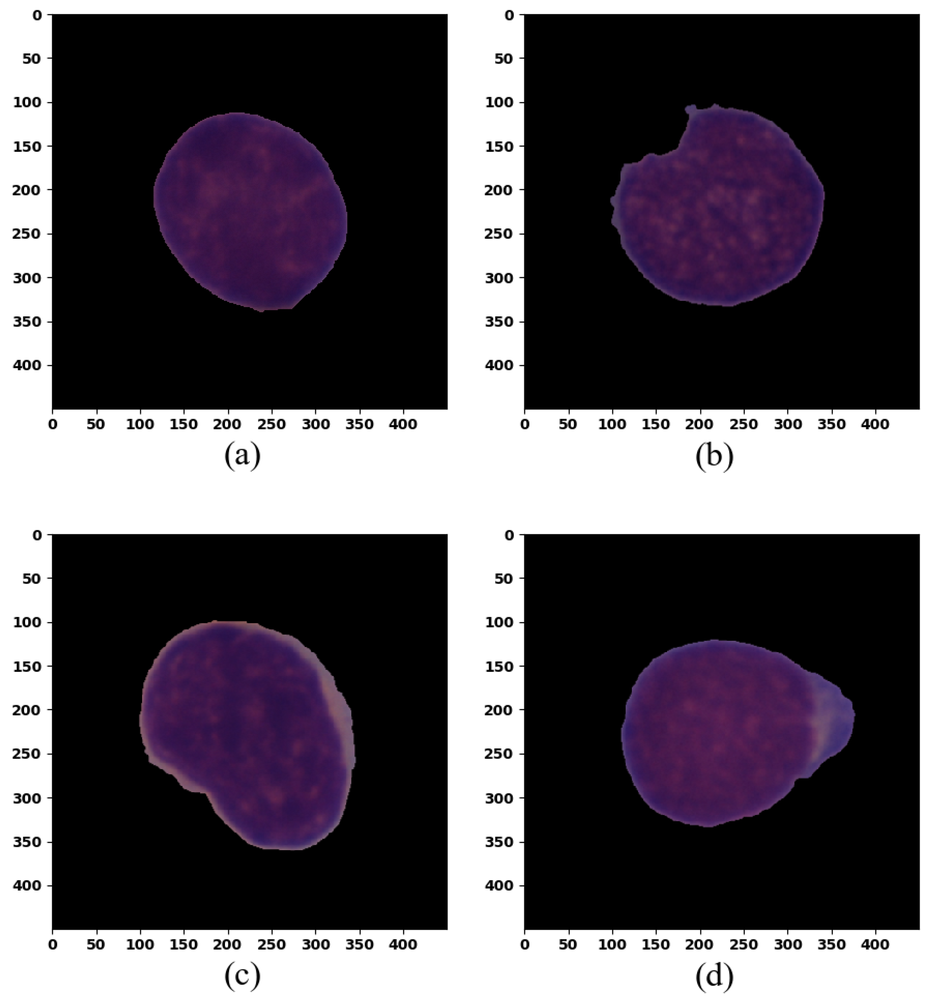
2.1. C-NMC 2019 Dataset
2.2. Data Augmentation
3. Feature Extraction
4. Ensemble Classifier
4.1. Naive Bayes Classifier
4.2. K-Nearest Neighbor
4.3. Support Vector Machine
4.4. Neural Network Training and Fine-Tuning
4.5. Ensemble Learning
- ANN + SVM + NB (full ensemble model, with best F1-score).
- ANN + SVM + KNN.
- ANN + KNN + NB.
- SVM + KNN + NB.
4.6. Principal Component Analysis and Interpretable Models
- PCA, ANN + SVM + NB (reduced ensemble model).
5. Results and Discussion
6. Conclusions and Future Work
Author Contributions
Funding
Data Availability Statement
Conflicts of Interest
References
- Hoffbrand, A.V.; Moss, P.A.H. Essential Haematology, 6th ed.; Wiley: Hoboken, NJ, USA, 2013. [Google Scholar]
- Instituto Nacional do Câncer. Tipos de Câncer: Leucemia. 2022. Available online: https://www.inca.gov.br/tipos-de-cancer/leucemia (accessed on 8 June 2022).
- Mishra, S.; Majhi, B.; Sa, P.K. Texture feature based classification on microscopic blood smear for acute lymphoblastic leukemia detection. Biomed. Signal Process. Control 2019, 47, 303–311. [Google Scholar] [CrossRef]
- Moshavash, Z.; Danyali, H.; Helfroush, M.S. An Automatic and Robust Decision Support System for Accurate Acute Leukemia Diagnosis from Blood Microscopic Images. J. Digit. Imaging 2018, 31, 702–717. [Google Scholar] [CrossRef] [PubMed]
- Labati, R.D.; Piuri, V.; Scotti, F. ALL-IDB: The Acute Lymphoblastic Leukemia Image Database for Image Processing. In Proceedings of the 18th IEEE International Conference on Image Processing (ICIP), Brussels, Belgium, 11–14 September 2011; pp. 2045–2048. [Google Scholar]
- DI-UNIMI. ALL-IDB: Acute Lymphoblastic Leukemia Image Database for Image Processing. 2020. Available online: https://homes.di.unimi.it/scotti/all/ (accessed on 8 June 2022).
- Putzu, L.; Caocci, G.; Ruberto, C.D. Leucocyte classification for leukaemia detection using image processing techniques. Artif. Intell. Med. 2014, 62, 179–191. [Google Scholar] [CrossRef] [PubMed]
- Mishra, S.; Sharma, L.; Majhi, B.; Sa, P.K. Microscopic Image Classification Using DCT for the Detection of Acute Lymphoblastic Leukemia (ALL). In Advances in Intelligent Systems and Computing; Springer: Singapore, 2016; pp. 171–180. [Google Scholar]
- MoradiAmin, M.; Memari, A.; Samadzadehaghdam, N.; Kermani, S.; Talebi, A. Computer aided detection and classification of acute lymphoblastic leukemia cell subtypes based on microscopic image analysis. Microsc. Res. Tech. 2016, 79, 908–916. [Google Scholar] [CrossRef] [PubMed]
- Shafique, S.; Tehsin, S. Acute Lymphoblastic Leukemia Detection and Classification of Its Subtypes Using Pretrained Deep Convolutional Neural Networks. Technol. Cancer Res. Treat. 2018, 17, 1533033818802789. [Google Scholar] [CrossRef] [PubMed]
- Mourya, S.; Kant, S.; Kumar, P.; Gupta, A.; Gupta, R. LeukoNet: DCT-based CNN architecture for the classification of normal versus Leukemic blasts in B-ALL Cancer. arXiv 2018, arXiv:1810.07961. [Google Scholar]
- Liu, D.; Cui, W.; Jin, K.; Guo, Y.; Qu, H. DeepTracker: Visualizing the Training Process of Convolutional Neural Networks. ACM Trans. Intell. Syst. Technol. 2018, 10, 6. [Google Scholar] [CrossRef]
- Garcia, N.F.; Tiggeman, F.; Borges, E.N.; Lucca, G.; Santos, H.; Dimuro, G. Exploring the relationships between data complexity and classification diversity in ensembles. In Proceedings of the 23rd International Conference on Enterprise Information Systems (ICEIS), Online, 26–28 April 2021. [Google Scholar]
- Abdar, M.; Makarenkov, V. CWV-BANN-SVM ensemble learning classifier for an accurate diagnosis of breast cancer. Measurement 2019, 146, 557–570. [Google Scholar] [CrossRef]
- Hsieh, S.L.; Hsieh, S.H.; Cheng, P.H.; Chen, C.H.; Hsu, K.P.; Lee, I.S.; Wang, Z.; Lai, F. Design ensemble machine learning model for bresat cancer diagnosis. J. Med. Syst. 2011, 36, 2841–2847. [Google Scholar] [CrossRef]
- Moon, W.K.; Lee, Y.W.; Ke, H.H.; Lee, S.H.; Huang, C.S.; Chang, R.F. Computer-aided diagnosis of breast ultrasound images using ensemble learning from convolutional neural networks. Comput. Methods Programs Biomed. 2020, 190, 105361. [Google Scholar] [CrossRef]
- Xiao, F.; Kuang, R.; Ou, Z.; Xiong, B. DeepMEN: Multi-model Ensemble Network for B-Lymphoblast Cell Classification. In Lecture Notes in Bioengineering; Springer: Singapore, 2019; pp. 83–93. [Google Scholar]
- Liu, Y.; Long, F. Acute Lymphoblastic Leukemia Cells Image Analysis with Deep Bagging Ensemble Learning. In Lecture Notes in Bioengineering; Springer: Singapore, 2019; pp. 113–121. [Google Scholar]
- Sant’Anna, Y.F.D.; Oliveira, J.E.M.; Dantas, D.O. Lightweight Classification of Normal Versus Leukemic Cells Using Feature Extraction. In Proceedings of the 2021 IEEE Symposium on Computers and Communications (ISCC), Athens, Greece, 5–8 September 2021; pp. 1–7. [Google Scholar] [CrossRef]
- van Griethuysen, J.J.M.; Fedorov, A.; Parmar, C.; Hosny, A.; Aucoin, N.; Narayan, V.; Beets-Tan, R.G.H.; Fillion-Robin, J.C.; Pieper, S.; Aerts, H.J. Computational Radiomics System to Decode the Radiographic Phenotype. Cancer Res. 2017, 77, e104–e107. [Google Scholar] [CrossRef]
- SBILab. Signal Processing and Biomedical Imaging Lab. 2022. Available online: http://sbilab.iiitd.edu.in/ (accessed on 8 June 2022).
- Mourya, S.; Kant, S.; Kumar, P.; Gupta, A.; Gupta, R. ALL Challenge Dataset of ISBI. 2019. Available online: https://wiki.cancerimagingarchive.net/x/zwYlAw (accessed on 8 June 2022).
- Marzahl, C.; Aubreville, M.; Voigt, J.; Maier, A. Classification of Leukemic B-Lymphoblast Cells from Blood Smear Microscopic Images with an Attention-Based Deep Learning Method and Advanced Augmentation Techniques. In Lecture Notes in Bioengineering; Springer: Singapore, 2019; pp. 13–22. [Google Scholar]
- Gupta, R.; Mallick, P.; Duggal, R.; Gupta, A.; Sharma, O. Stain Color Normalization and Segmentation of Plasma Cells in Microscopic Images as a Prelude to Development of Computer Assisted Automated Disease Diagnostic Tool in Multiple Myeloma. Clin. Lymphoma Myeloma Leuk. 2017, 17, e99. [Google Scholar] [CrossRef]
- Duggal, R.; Gupta, A.; Gupta, R.; Wadhwa, M.; Ahuja, C. Overlapping cell nuclei segmentation in microscopic images using deep belief networks. In Proceedings of the Tenth Indian Conference on Computer Vision, Graphics and Image Processing (ICVGIP), Guwahati, India, 18–22 December 2016; ACM Press: New York, NY, USA, 2016. [Google Scholar]
- Duggal, R.; Gupta, A.; Gupta, R.; Mallick, P. SD-Layer: Stain Deconvolutional Layer for CNNs in Medical Microscopic Imaging. In Proceedings of the Medical Image Computing and Computer Assisted Intervention (MICCAI), Quebec City, QC, Canada, 11–13 September 2017; Springer: Cham, Switzerland, 2017; pp. 435–443. [Google Scholar]
- SBILab. Classification of Normal vs Malignant Cells in B-ALL White Blood Cancer Microscopic Images: ISBI 2019. 2019. Available online: https://competitions.codalab.org/competitions/20395 (accessed on 8 June 2022).
- Jacobusse, G.; Veenman, C. On Selection Bias with Imbalanced Classes. In Proceedings of the International Conference on Discovery Science, Kyoto, Japan, 15–17 October 2016; pp. 325–340. [Google Scholar] [CrossRef]
- Zwanenburg, A.; Leger, S.; Vallières, M.; Löck, S. Image Biomarker Standardisation Initiative. arXiv 2016, arXiv:1612.07003. [Google Scholar]
- Aggarwal, N.; Agrawal, R.K. First and Second Order Statistics Features for Classification of Magnetic Resonance Brain Images. J. Signal Inf. Process. 2012, 3, 146–153. [Google Scholar] [CrossRef]
- Houby, E.M.F.E. Framework of Computer Aided Diagnosis Systems for Cancer Classification Based on Medical Images. J. Med. Syst. 2018, 42, 157. [Google Scholar] [CrossRef]
- Cosgriff, R.L. Identification of Shape; Technical Report, Report 820-11; Ohio State University Research Foundation: Columbus, OH, USA, 1960. [Google Scholar]
- Alhilal, M.S.; Soudani, A.; Al-Dhelaan, A. Image-Based Object Identification for Efficient Event-Driven Sensing in Wireless Multimedia Sensor Networks. Int. J. Distrib. Sens. Netw. 2015, 11, 850–869. [Google Scholar] [CrossRef]
- Klinzmann, A.; Bhonsle, S. Centroid Distance Function and the Fourier Descriptor with Applications to Cancer Cell Clustering; Technical Report; UCI Department of Mathematics: Irvine, CA, USA, 2011. [Google Scholar]
- Wu, Y.G. Medical image compression by sampling DCT coefficients. IEEE Trans. Inf. Technol. Biomed. 2002, 6, 86–94. [Google Scholar]
- Vishwakarma, V.P.; Pandey, S.; Gupta, M. A Novel Approach for Face Recognition Using DCT Coefficients Re-scaling for Illumination Normalization. In Proceedings of the 15th International Conference on Advanced Computing and Communications (ADCOM), Guwahati, India, 18–21 December 2007; pp. 535–539. [Google Scholar]
- Kubat, M. An Introduction to Machine Learning, 2nd ed.; Springer International Publishing: Cham, Switzerland, 2017. [Google Scholar]
- Duda, R.O.; Hart, P.E.; Stork, D.G. Pattern Classification, 2nd ed.; Wiley: New York, NY, USA, 2001. [Google Scholar]
- Kingma, D.P.; Ba, J. Adam: A Method for Stochastic Optimization. In Proceedings of the International Conference on Learning Representations, San Diego, CA, USA, 7–9 May 2015. [Google Scholar]
- Dietterich, T.G. Ensemble Learning, 6th ed.; The MIT Press: Cambridge, MA, USA, 2002. [Google Scholar]
- Mohandes, M.; Deriche, M.; Aliyu, S.O. Classifiers Combination Techniques: A Comprehensive Review. IEEE Access 2018, 6, 19626–19639. [Google Scholar] [CrossRef]
- Soriano, A.; Vergara, L.; Ahmed, B.; Salazar, A. Fusion of Scores in a Detection Context Based on Alpha Integration. Neural Comput. 2015, 27, 1983–2010. [Google Scholar] [CrossRef]
- Safont, G.; Salazar, A.; Vergara, L. Vector score alpha integration for classifier late fusion. Pattern Recognit. Lett. 2020, 136, 48–55. [Google Scholar] [CrossRef]
- Ruding, C. Stop explaining black box machine learning models for high stakes decisions and use interpretable models instead. Nat. Mach. Intell. 2019, 1, 206–215. [Google Scholar] [CrossRef]
- Raschka, S. SequentialFeatureSelector: The Popular Forward and Backward Feature Selection Approaches Incl. Floating Variants. 2020. Available online: http://rasbt.github.io/mlxtend/user_guide/feature_selection/SequentialFeatureSelector/ (accessed on 8 June 2022).
- Gupta, A.; Gupta, R. (Eds.) ISBI 2019 C-NMC Challenge: Classification in Cancer Cell Imaging; Springer: Singapore, 2019. [Google Scholar]
- Pan, Y.; Liu, M.; Xia, Y.; Shen, D. Neighborhood-Correction Algorithm for Classification of Normal and Malignant Cells. In Lecture Notes in Bioengineering; Springer: Singapore, 2019; pp. 73–82. [Google Scholar]
- Honnalgere, A.; Nayak, G. Classification of Normal Versus Malignant Cells in B-ALL White Blood Cancer Microscopic Images. In Lecture Notes in Bioengineering; Springer: Singapore, 2019; pp. 1–12. [Google Scholar] [CrossRef]
- Verma, E.; Singh, V. ISBI Challenge 2019: Convolution Neural Networks for B-ALL Cell Classification. In Lecture Notes in Bioengineering; Springer: Singapore, 2019; pp. 131–139. [Google Scholar]
- Prellberg, J.; Kramer, O. Acute Lymphoblastic Leukemia Classification from Microscopic Images Using Convolutional Neural Networks. In Lecture Notes in Bioengineering; Springer: Singapore, 2019; pp. 53–61. [Google Scholar]
- Shah, S.; Nawaz, W.; Jalil, B.; Khan, H.A. Classification of Normal and Leukemic Blast Cells in B-ALL Cancer Using a Combination of Convolutional and Recurrent Neural Networks. In Lecture Notes in Bioengineering; Springer: Singapore, 2019; pp. 23–31. [Google Scholar]
- Ding, Y.; Yang, Y.; Cui, Y. Deep Learning for Classifying of White Blood Cancer. In Lecture Notes in Bioengineering; Springer: Singapore, 2019; pp. 33–41. [Google Scholar]
- Kulhalli, R.; Savadikar, C.; Garware, B. Toward Automated Classification of B-Acute Lymphoblastic Leukemia. In Lecture Notes in Bioengineering; Springer: Singapore, 2019; pp. 63–72. [Google Scholar]
- Khan, M.A.; Choo, J. Classification of Cancer Microscopic Images via Convolutional Neural Networks. In Lecture Notes in Bioengineering; Springer: Singapore, 2019; pp. 141–147. [Google Scholar]
- de Oliveira, J.E.M.; Dantas, D.O. Classification of Normal versus Leukemic Cells with Data Augmentation and Convolutional Neural Networks. In Proceedings of the 16th International Joint Conference on Computer Vision, Imaging and Computer Graphics Theory and Applications, VISAPP, INSTICC, Online, 8–10 February 2021; SciTePress: Setúbal Municipality, Portugal, 2021; Volume 4, pp. 685–692. [Google Scholar] [CrossRef]
- Pepe, M.S. The Statistical Evaluation of Medical Tests for Classification and Prediction; Oxford Statistical Sciences Series; Oxford University Press: New York, NY, USA, 2003. [Google Scholar]
- Metrock, L.K.; Summers, R.J.; Park, S.; Gillespie, S.; Castellino, S.; Lew, G.; Keller, F.G. Utility of peripheral blood immunophenotyping by flow cytometry in the diagnosis of pediatric acute leukemia. Pediatr. Blood Cancer 2017, 64, e26526. [Google Scholar] [CrossRef]
- Lam, G.; Punnett, A.; Stephens, D.; Sung, L.; Abdelhaleem, M.; Hitzler, J. Value of flow cytometric analysis of peripheral blood samples in children diagnosed with acute lymphoblastic leukemia. Pediatr. Blood Cancer 2018, 65, e26738. [Google Scholar] [CrossRef]
- Beltrame, M.P.; Souto, E.X.; Yamamoto, M.; Furtado, F.M.; Costa, E.S.; Sandes, A.F.; Pimenta, G.; Cavalcanti Júnior, G.B.; Santos-Silva, M.C.; Lorand-Metze, I.; et al. Updating recommendations of the Brazilian Group of Flow Cytometry (GBCFLUX) for diagnosis of acute leukemias using four-color flow cytometry panels. Hematol. Transfus. Cell Ther. 2021, 43, 499–506. [Google Scholar] [CrossRef]
- Safont, G.; Salazar, A.; Vergara, L. New Applications of Late Fusion Methods for EEG Signal Processing. In Proceedings of the 2019 International Conference on Computational Science and Computational Intelligence (CSCI), Las Vegas, NV, USA, 15–17 December 2019; pp. 617–621. [Google Scholar] [CrossRef]
- Amari, S. Integration of Stochastic Models by Minimizing alpha-Divergence. Neural Comput. 2007, 19, 2780–2796. [Google Scholar] [CrossRef]


| Original | Data-Augmentation | |||
|---|---|---|---|---|
| Malignant | Healthy | Malignant | Healthy | |
| Training | 5923 (42) | 3035 (29) | 20,000 | 20,000 |
| Validation | 1531 (12) | 506 (8) | 5000 | 5000 |
| Test | 1007 (6) | 496 (4) | N/A | N/A |
| Feature Type | Number |
|---|---|
| Low-order statistical | 108 |
| Textural | 75 |
| Morphological | 20 |
| Contour | 160 |
| DCT | 1024 |
| Total | 1387 |
| Parameter | Values | Chosen Value |
|---|---|---|
| Hidden Layers | 1, 2, 3, 4 | 1 |
| Batch Size | 250, 750, 1000, 1500 | 250 |
| Dropout | 0.1, 0.25, 0.3, 0.5 | 0.1 |
| Neurons Number | 1024, 1536, 2048, 2560 | 2560 |
| Activation | Prelu, Relu, Sigmoid, Softmax | Relu |
| Optimizer | Adamax, Adam, SGD | Adam |
| Kernel Initializer | Random Uniforme, Normal | Normal |
| Feature Type | Number |
|---|---|
| Low-order statistical | 33 |
| Textural | 45 |
| Morphological | 4 |
| Contour | 4 |
| DCT | 182 |
| Total | 268 |
| SBILab Challenger | F1-Score | Methodology |
|---|---|---|
| ANN + SVM + NB | 93.70% | Feature extraction and ensemble classifier |
| [47] | 92.50% | Transfer learning with ResNets |
| [48] | 91.70% | Transfer learning with VGG16 |
| ANN + SVM + KNN | 91.80% | Feature extraction and ensemble classifier |
| ANN | 91.20% | Feature extraction and ANN |
| ANN + KNN + NB | 90.60% | Feature extraction and ensemble classifier |
| [17] | 90.30% | Deep multi-model ensemble network |
| PCA, ANN + SVM + NB | 89.87% | Reduced feature vector and ensemble classifier |
| [49] | 89.47% | Transfer learning with MobileNetV2 |
| [50] | 87.89% | ResNeXt50 |
| SVM + KNN + NB | 87.60% | Feature extraction and ensemble classifier |
| [51] | 87.58% | Transfer learning with CNN and recurrent ANN |
| [23] | 87.46% | Transfer learning with ResNet18 |
| [52] | 86.74% | InceptionV3 + DenseNet + InceptionResNetV2 |
| [53] | 85.70% | ResNeXt50 + ResNeXt101 |
| [18] | 84.00% | Transfer learning with Inception + ResNets |
| [54] | 81.79% | Transfer learning with ResNets + SENets |
| SVM | 79.53% | Feature extraction and SVM |
| KNN | 76.66% | Feature extraction and KNN |
| NB | 74.25% | Feature extraction and NB |
| Network | Number of Parameters |
|---|---|
| VGG16 | 138,357,544 |
| ResNet152 | 60,380,648 |
| InceptionResNetV2 | 55,873,736 |
| ResNet50 | 25,636,712 |
| Xception | 22,910,480 |
| DenseNet201 | 20,242,984 |
| ANN and full ensemble | 9,177,601 |
| DenseNet121 | 8,062,504 |
| Reduced ensemble model | 2,775,553 |
| Metric | Reduced Ensemble | ANN | Full Ensemble | VGG16 |
|---|---|---|---|---|
| Feature extraction time | 16 min | 1 h 2 min | 1 h 2 min | - |
| Training time | 8 min | 9 min | 9 min | 16 h 20 min |
| Number of parameters | 2,775,553 | 9,177,601 | 9,177,601 | 66,358,593 |
| F1-score | 89.87% | 91.20% | 93.70% | 92.60% |
| Metric | Reduced Ensemble | ANN | Full Ensemble |
|---|---|---|---|
| F1-Score | 89.87% | 91.20% | 93.70% |
| Accuracy | 83.19% | 86.82% | 88.13% |
| Sensitivity | 86.60% | 88.11% | 95.47% |
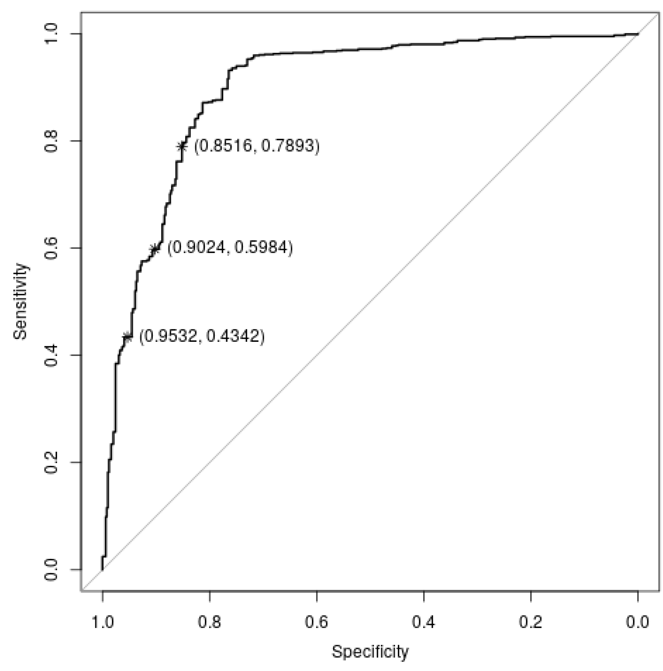
| AUC | 75.10% | 84.68% | 88.36% |
| Kappa | 44.47% | 56.45% | 67.79% |
| Precision | 94.36% | 96.48% | 97.32% |
| Specificity | 65.43% | 77.92% | 80.25% |
| Metric | Reduced Ensemble Mean (SD) | Reduced vs. ANN p-Value | ANN Mean (SD) | ANN vs. Full p-Value | Full Ensemble Mean (SD) |
|---|---|---|---|---|---|
| F1-Score | 89.78% (0.74%) | 1.6 × 10⁻³¹ | 91.94% (0.75%) | 1.0 × 10⁻²⁴ | 93.88% (1.41%) |
| Accuracy | 83.05% (1.16%) | 6.7 × 10⁻³² | 86.54% (1.19%) | 1.1 × 10⁻²⁴ | 89.67% (2.32%) |
| Sensitivity | 85.24% (1.13%) | 9.8 × 10⁻²⁸ | 87.89% (1.18%) | 9.2 × 10⁻²⁵ | 90.89% (2.21%) |
| AUC | 76.62% (1.99%) | 1.3 × 10⁻³² | 82.57% (1.94%) | 3.2 × 10⁻¹⁷ | 86.12% (3.02%) |
| Kappa | 40.99% (3.40%) | 1.2 × 10⁻³² | 51.79% (3.53%) | 2.2 × 10⁻²³ | 61.08% (7.64%) |
| Precision | 94.85% (0.58%) | 2.6 × 10⁻³⁴ | 96.38% (0.56%) | 2.6 × 10⁻³⁴ | 97.09% (0.72%) |
| Specificity | 68.01% (3.57%) | 2.3 × 10⁻³¹ | 77.25% (3.48%) | 2.1 × 10⁻¹⁰ | 81.35% (4.41%) |
Publisher’s Note: MDPI stays neutral with regard to jurisdictional claims in published maps and institutional affiliations. |
© 2022 by the authors. Licensee MDPI, Basel, Switzerland. This article is an open access article distributed under the terms and conditions of the Creative Commons Attribution (CC BY) license (https://creativecommons.org/licenses/by/4.0/).
Share and Cite
de Sant’Anna, Y.F.D.; de Oliveira, J.E.M.; Dantas, D.O. Interpretable Lightweight Ensemble Classification of Normal versus Leukemic Cells. Computers 2022, 11, 125. https://doi.org/10.3390/computers11080125
de Sant’Anna YFD, de Oliveira JEM, Dantas DO. Interpretable Lightweight Ensemble Classification of Normal versus Leukemic Cells. Computers. 2022; 11(8):125. https://doi.org/10.3390/computers11080125
Chicago/Turabian Stylede Sant’Anna, Yúri Faro Dantas, José Elwyslan Maurício de Oliveira, and Daniel Oliveira Dantas. 2022. "Interpretable Lightweight Ensemble Classification of Normal versus Leukemic Cells" Computers 11, no. 8: 125. https://doi.org/10.3390/computers11080125
APA Stylede Sant’Anna, Y. F. D., de Oliveira, J. E. M., & Dantas, D. O. (2022). Interpretable Lightweight Ensemble Classification of Normal versus Leukemic Cells. Computers, 11(8), 125. https://doi.org/10.3390/computers11080125